Abstract
A nonlinear adaptive multiple-input multiple-output (NAMIMO) controller is designed to control a super capacitor compensation inverter. The proposed controller effectively suppresses the effects of impact loads from natural gas generation systems. In this paper, the transient current model of the compensation system is transformed into the power model using transient power theory, and then a direct power control algorithm with a vector control strategy is designed based on the whole power model. The proposed strategy can not only effectively suppress the impact of impact loads on the system but also maintain the stability of the microgrid to a certain extent. Meanwhile, the PLL control structure is replaced by an adaptive algorithm, which not only solves the system instability problem but also improves the dynamic response of the compensation system. In addition, the functional advantages, the frequency is bounded and stable throughout the whole process, and this differential frequency modulation allows the compensation system to exit the compensation smoothly. Finally, the simulation and experimental results on a 600 kW natural gas generator demonstrate that the proposed compensation strategy and control algorithm can effectively suppress the impact load effects.
1. Introduction
The microgrid composed of internal combustion engines and distributed power sources has attracted much attention for its flexible application scenarios. Meanwhile, natural gas as a fuel for generators mitigates the growing energy crisis [1]. In microgrids, it is very important to ensure the transient stability of natural gas generators, especially after the generators are subjected to impact loads [2]. In contrast to conventional loads, impact loads exhibit impact and cyclic operating modes, while their peak power is much higher than the average power. For natural gas generators, if their power angle or relative speed deviates too much from the operating point, it will lead to the loss of synchronization between the generator and the microgrid or even damage the rotor [3]. However, high-power internal combustion engines usually have a large moment of inertia. Therefore, the generator cannot satisfy the power balance of the grid at the moment when the impact load is connected. Engineers and researchers have conducted a lot of research to solve this problem in terms of control strategies and internal gas structures [4,5].
In the last few decades, many researchers have believed that the moment the microgrid is impacted, an additional energy storage device must be used to release the energy required by the load [6,7]. The most widely used forms of energy storage include lithium batteries [8], super capacitors [9,10], flywheel energy storage [11,12,13], and superconducting magnetic energy storage [14,15], etc. Among them, the safety of flywheel energy storage severely restricts its development, and the lithium battery has high requirements for ambient temperature. Although the energy density of super capacitors is lower than that of lithium batteries, they have a high power density, are maintenance-free, have a long service life, and have a wide range of applicable temperatures [16]. Therefore, super capacitors can be effectively used as an energy source for impact load compensation devices. Moreover, the impact load compensation trouble turns into the problem of control strategies for super capacitor compensation devices to achieve fast power response.
The grid-connected inverters currently have two main control modes. One is to directly control the d-q axis current to regulate its grid-connected power while using a phase-locked loop to obtain the grid voltage phase [17]; this control method can equate the grid-connected inverter as a current source [18]. The other one is to regulate the grid-connected power directly by controlling the vector and phase of the output voltage, whose active power and reactive power are similar to the synchronous generator system in relation to the phase and amplitude of the voltage. In Bouafia et al. [19], the authors propose a voltage-source inverter that does not use a PLL and has good stability in weak grids. For now, the voltage-source mode is usually based on droop control or a virtual synchronous generator to simulate the electromagnetic characteristics of an actual synchronous generator. Then, the vector amplitude and phase of the output voltage are regulated by the power outer loop, which in turn regulates the output power. In Meng et al. [20], the authors review the conventional droop control and virtual synchronous generator techniques, and a generalized droop control method for grid-connected inverters is proposed on this basis. This proposed generalized sag control has a flexible active power control loop to meet various types of loads. In Dong et al. [21], authors analyze the stability of the virtual synchronous generation technique at high line impedances. The results of the paper demonstrate that the voltage source mode is more stable than the current source mode under weak grids. Current-source grid-connected inverters usually use control strategies such as grid voltage feedforward and PLL. However, the fluctuation of grid impedance caused by load throwing will not only reduce the stability margin of the inverter but also cause harmonic resonance or even instability of the inverter [22]. The main cause of this phenomenon is the use of phase phase-locked loop in the current source. In Dong et al. [21], the authors proposed a nonlinear PLL, and their conclusions showed that impedance fluctuations can cause self-synchronization phenomena in the PLL, which can lead to inverter instability. Wang et al. [23] proposed a unified impedance model for grid-connected inverters, and their conclusions showed that a higher PLL bandwidth would lead to harmonic resonance in weak grids. In summary, current-source inverters are suitable for strong grids, while their stability is reduced under weak grids and even unstable under very weak grids. On the contrary, voltage-source inverters in a weak grid have better stability, while the system is not stable in a strong grid. Therefore, the voltage-source mode is chosen for energy compensation in this paper.
The virtual synchronous generator (VSG) is a voltage-based converter that has been widely used in the field of new energy generation [24]. It can simulate the inertia and damping characteristics of conventional synchronous generators. VSGs applied in distributed generation have the following characteristics [25]. First, a VSG can provide inertia support to microgrids, which helps to reduce the frequency deviation when load changes or faults occur. Second, compared with the traditional voltage source converter, the operation of a VSG does not depend on the phase angle of the microgrid voltage, which avoids the instability problem due to the phase-locked loop (PLL) [26]. In addition, the VSG achieves frequency and voltage droop control through its active power–frequency control and reactive power–voltage control, thus improving power angle stability and system voltage stability by using only local communication.
For voltage source inverters, in addition to the droop control and virtual synchronous control mentioned above, direct power control has attracted the attention of scholars because of its simple algorithm structure and high power factor [27,28]. Note that the power equation of the inverter side in this paper is borrowed from the literature [27]. In the conventional direct power control method, not only is a large amount of tuning required, but large harmonics of the bus voltage can also occur in the presence of grid impedance distortion. Zhang et al. [29] proposed an online inductance identification technique based on the gradient correction method based on extended power theory and combined it with DPC to improve the robustness of DPC. Sato et al. [30] proposed a control strategy for a voltage source pulse-width modulated (PWM) rectifier inverter based on direct power control. Although the proposed DPC technique can fully regulate the stability of the output current without special compensation blocks, its experimental results show that its output current has a certain degree of distortion. Therefore, we design and propose the control strategy of the compensation device based on direct power control.
After analyzing the above discussion, in this paper, we present a controller scheme: (i) transforming the transient mathematical model of the voltage-source PWM inverter into a power model, with the help of transient power theory; (ii) designing adaptive frequency controller to implement the frequency tracking control; (iii) designing the NAMIMO controller to control compensation device to compensate impact loads.
The contributions of this paper are as follows: (i) we designed a NAMIMO controller to implement impact load compensation for natural gas generators; (ii) The frequency adaptive law of the controller not only improved power transient response characteristics but also realized power differential regulation.
This paper is organized below. Section 2. mainly establishes the direct power model of the compensation system and the generator system. Meanwhile, the open-loop dynamic characteristics of the compensation system are described in this section. Section 3. explains the design process of the NAMIMO control algorithm and shows the stability proof of the whole system. The simulated and experimental waveforms are displayed in Section 4., and the corresponding analysis and discussion are in this chapter. Finally, the work of this paper is summarized, and the conclusions are shown in Section 5.
2. Mathematical Models
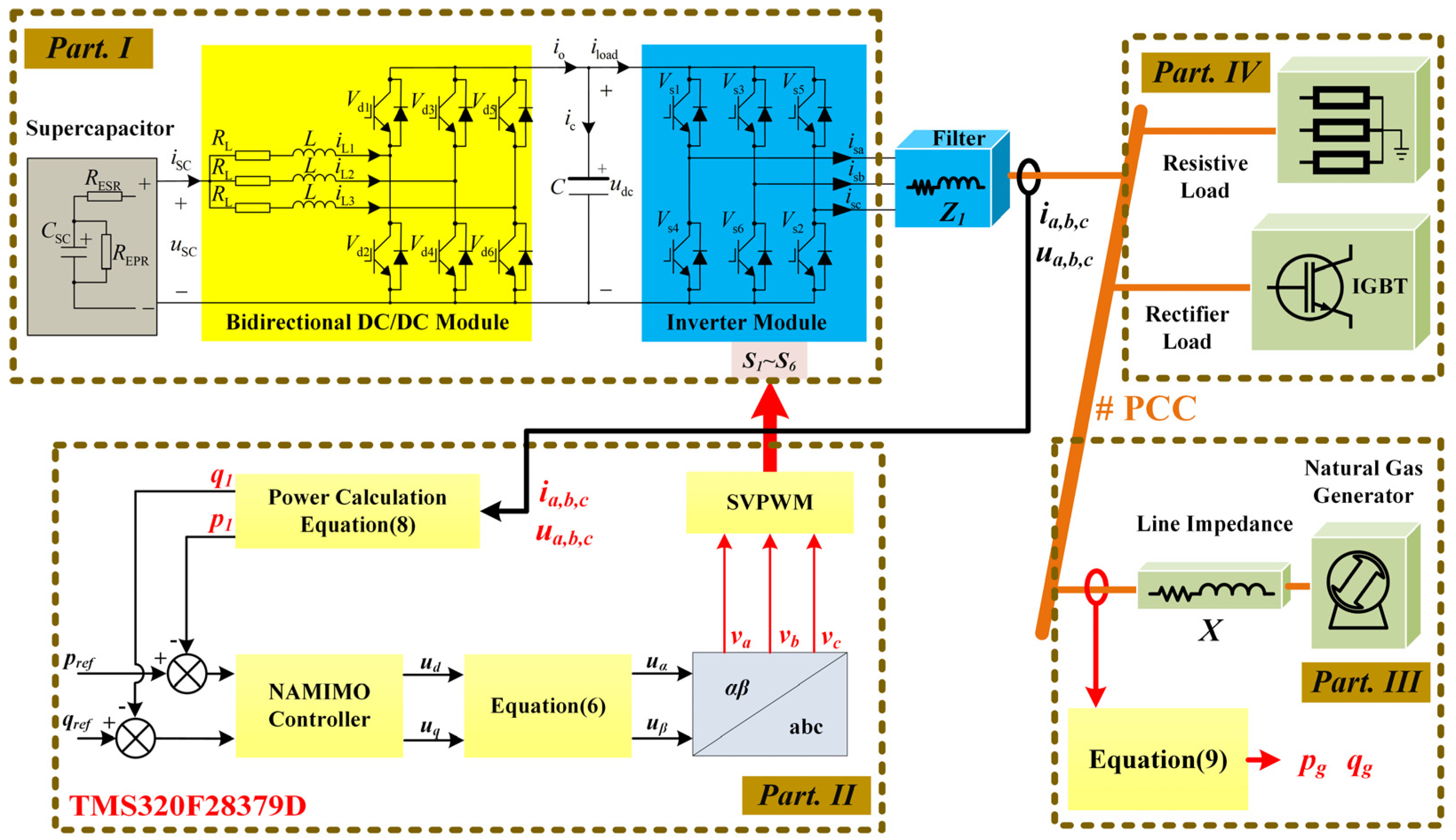
In this section, first, to investigate the super capacitor compensation-based natural gas generator system, a mathematical model of the aggregate parameters is established to represent the current and power relationships of the system. The structure of the whole compensation system is shown in part I of Figure 1. The compensation system contains a super capacitor compensation device, PWM inverters, a generator, and an impact load. Moreover, three assumptions have been asserted on the compensation system in this paper:
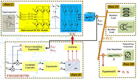
Figure 1.
Power generation system architecture and its system control block diagram.
A1: Capacitive voltage on the DC side of the inverter is constant.
A2: Ignore the loss of power electronics in the system itself.
A3: The bus voltage is a symmetrical three-phase voltage.
2.1. Mathematical Model of Compensation System Output Power
As shown in Figure 1, a three-phase, three-wire, two-level PWM inverter is constructed to implement the power conversion in the compensation system. Super capacitors and DC–DC converters are used as the DC side power supply of the inverter. Note that this paper assumes that the capacitive voltage on the DC side of the inverter is constant. The state-space equations consist of the output voltage and current of the compensated system, as well as the grid-side bus voltage, are as follows:
where abc is subscripts of the ABC coordinate system. R1 and L1 are the resistance and inductance of the RL filter, respectively. ua, ub, and uc stand for the phase voltage of the grid-side bus. i1a, i1b, and i1c are line currents of the inverter. udc represents the DC bus voltage of the inverter. Sa,b,c is the switching function of the inverter bridge arms.
Equation (1) is converted to the α-β stationary coordinate system as follows:
where α and β are the subscripts of the αβ coordinate system. u1α and u1β are the phase voltage of the inverter. i1α and i1β are the line currents of the inverter. sα and sβ are Switching functions of the inverter bridge arms in the αβ coordinate system.
Conventional power is not only based on the premise that voltage and current are periodically varying quantities but it is also calculated based on the average value of power. Conventional power cannot make a correct description when the voltage and current are distorted. Therefore, this thesis constructs the transient power equation as follows:
where uα and uβ are the phase voltages of the grid-side bus, p1 and q1 stand for active and reactive power of the inverter output, respectively, and the length of q is as follows:
Next, substituting (2) and (3) into (4) and calculating the derivative of real and reactive powers. Finally, the equation obtained as follows [27]:
where
Substituting (6) into (4) to obtain the output power equation of the compensation system as follows:
where dpf and dqf are considered to be a power disturbance from the AC bus. Equation (7) explains the active and reactive power output of the compensation system in the d-q coordinate system.
2.2. Mathematical Model of Generation Output Power
The generation system consists of transmission line impedance and a natural gas generator. The single-equivalent circuit from the generator to the PCC point is shown in Figure 1III. In this paper, it is assumed that the line impedance between the generator and the PCC point is mainly inductive, which means the inductance is much greater than the resistance. Therefore, the active and reactive power output from the generator to the PCC point can be expressed as (8), respectively.
where pg and qg stand for the active and reactive power of the generator, Ug is the voltage amplitude of the generator, Um is the voltage amplitude of the grid bus, and δ is the power angle of the generator.
The generator terminal voltage and PCC point voltage are approximately equal to a constant when the system is steady state. Therefore, linearizing this equation at the stabilization point of the system as follows:
Calculating (8) to find its derivative function as follows:
Since (10) is linearized at the fixed point of the generator, the equation does not appear to include the control input signal. This does not mean that the output power of the generator during stabilization is a constant value. Because the voltage of the generator varies according to the excitation system. Note that the excitation system is not considered, and the generator output power is considered with bus frequency in this paper. According to (10), the generator power is constant when its speed no longer varies, such that
Equation (10) is brought into (7) as a disturbance term. The dynamic equation of the compensation system can be expressed as Equation (12).
2.3. Dynamic Characteristics Analysis of Open Loop System
The dynamic behavior of the compensation power is analyzed by means of the open loop power state equation of the compensation system. This provides a clear understanding of the power flow of the compensation system while designing power compensation control algorithms that adapt to load changes. First, (12) is rewritten in the compact state space form as:
where
Second, the constant solution (fixed point) of the compensated system is calculated as (14), and the eigenvalues of the open-loop state matrix of the compensation system are calculated as (15).
Equation (14) indicates that there is an equilibrium point in the system in case the denominator of the equation is not zero. However, there is the term in (15), so the system is not necessarily convergent. In this section, two cases of eigenvalues are considered as follows:
Case 1: R/L > ω. The voltage frequency of the generator is 50 Hz, so it is assumed that the actual value of ω is also approximately equal to 100π rad/s. Therefore, the case holds when the line resistance and filter inductance satisfy a 314-fold relationship. It can be inferred from (15) that the eigenvalues (, ) of the state matrix are all less than zero. Overall, the output power (, ) of the compensation system converges to the equilibrium point (, ) as time goes to infinity.
Case 2: R/L < ω. In this case, the range of eigenvalues (, ) is difficult to determine and leads to the system no longer converges. Therefore, the compensation system requires an additional controller. The added controller not only changes the eigenvalues of the state matrix but also makes the output power of the system converge to the new equilibrium point (, ). According to the above two categories of analysis, line impedance and filter have a crucial role in the stability of the system. To complicate matters further, it is also coupled to the frequency of the generator. Note that, the relationship between impedance and frequency is not continued to be considered in this paper.
3. Control Strategies
A nonlinear adaptive multiple-input and multiple-output (NAMIMO) controller has been proposed to control the output power of the compensation system. The biggest difficulty with the proposed controller is that the compensation system has to achieve minimal or no fluctuations in frequency. Meanwhile, it makes it more difficult to obtain frequency parameters for the system without PLL in this paper.
3.1. Description of the Closed-Loop System
The compensation system does not transmit power outward during stable operation. Hence, the compensation power is equal to zero when the impact load action is completed. As a result, to achieve the power tracking control, define two error control signals as follows:
where and represent the reference values of the output power of the compensation system, respectively. According to the analysis above, the reference value is considered to be equal to zero. These two signals ensure that the power can converge to the reference value in a finite time.
Meanwhile, another control objective of this thesis is to achieve frequency tracking control, so the third error control signal is designed as follows:
Next, solving the time derivative of (17) and substituting (12) into it, such that
where and represent the two control inputs of the system, respectively.
3.2. NAMIMO Controller Design and Stability Analysis
Equation (18) is the state space equation of the compensated system, and the design procedure is elaborated as follows:
Step 1: Create a Lyapunov function equation that includes all error signals as follows:
where α is defined as the adaptive control rate parameter, then calculate the dynamic equation of the (19) as follows:
According to the Lyapunov stability theory, (20) must be a negative definite function to ensure that the system is asymptotically stable. Therefore, the feedback linearization of (20) is performed in this step. The linearization function is as follows:
where
Step 2: Substituting (21), (22), (23), and (24) into (20), the dynamics of V is derived as
In order for (25) to be a negative definite function, the last term of the equation must be equal to zero. Thus, a turning function ϕ is defined as follows:
and the adaptive law of ω is shown below:
Step 3: Substituting (26) and (27) into (25), the Lyapunov function can be reduced to (28).
where k1 and k2 are controller gains. Note that (28) is a semi-negative function. Therefore, the stability of the compensation system cannot be directly derived from (28). Now, the system stability of the NAMIMO controller needs to be demonstrated.
First, writing (28) in compact form as follows:
Define the error vector as:
Due to:
Equation (29) can be translated as follows:
where and are controller gains, and is a symmetric positive definite matrix.
Then, analyzing and integrating the inequality as follows:
where
Substituting (33) and (34) into (32), such that:
The Lyapunov function (19) indicates V is a positive definite radially unbounded and decrescendo. This means that all variables within the function are bounded. As a summary, an inequality can be obtained as follows:
Second, bringing (36) into (35) yields a new inequality as:
Meanwhile, according to the analysis above, the following conditions hold:
.
As a result, the following extrapolation is proven:
Finally, according to Barbalat Lemma [31], we have a conclusion as follows:
Overall, although (28) shows that the Lyapunov function is semi-negative, equation (38) proves that the whole system is asymptotically stable. This means that two power control objectives of the system can converge to the reference value.
4. Simulation and Experimental Results Analysis
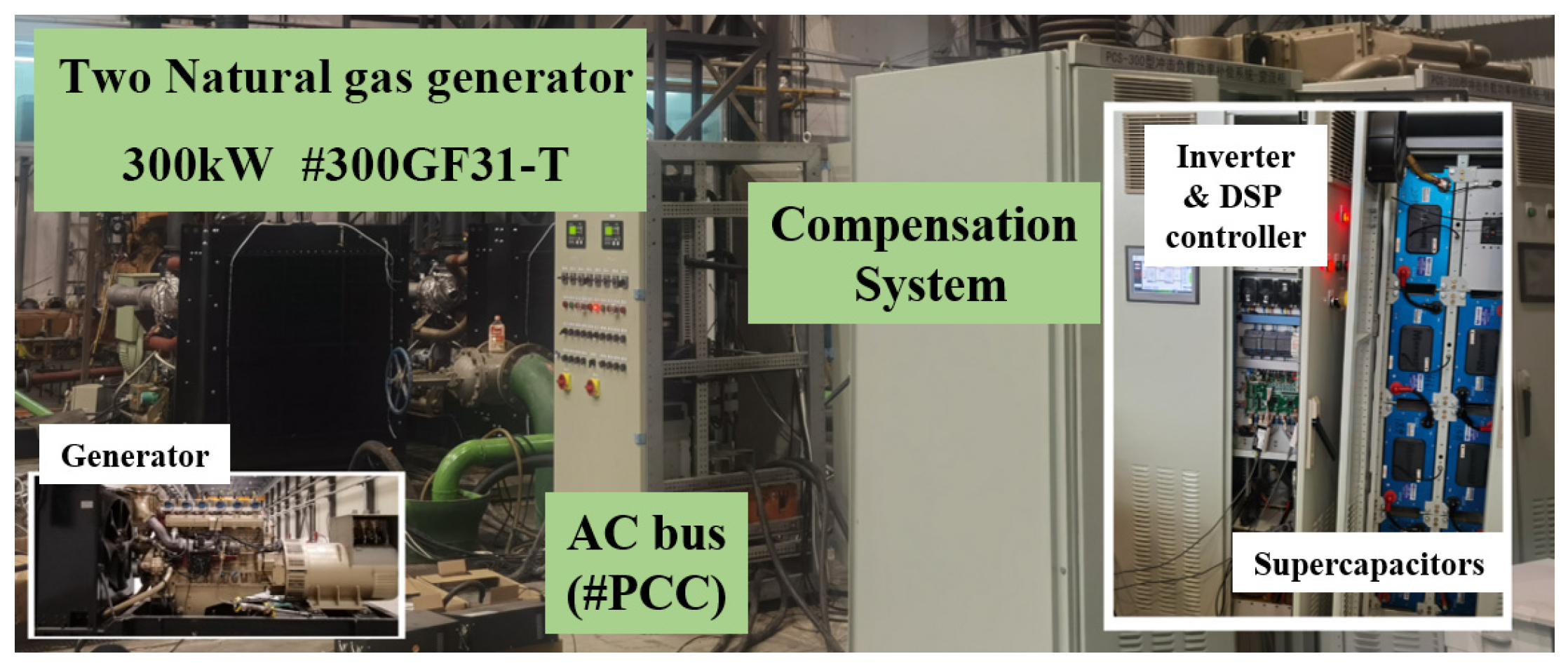
The simulation and experimental test platforms were created to evaluate the performance of the proposed control strategies. The simulation testbed is constructed in the RT-BOX3/PLECS environment. RT-Box3 is used as a real-time simulator for the power unit. The F38379D LaunchPad manufactured by TI is used as a control board to implement the proposed compensation strategy. LaunchPad and RT-Box3 are connected through the RT-Box LaunchPad. The HIL block diagram of the co-simulation between RT-Box3 and F28379D LaunchPad is shown in Figure 1. The whole HIL system is divided into two parts: the control unit and the power supply circuit. These two parts are loaded into the F28379D LaunchPad and RT-Box3 through PLECS (Version 4.7) software, respectively. Meanwhile, in order to more clearly characterize the compensation performance of the proposed strategy, a microgrid without a compensation device is set up as a control group. Figure 1 shows the block diagram of the natural gas generator system based on super capacitor compensation device. Its main components are as follows: (i) two natural gas generators (300GF31-T), its main parameters are displayed in Table 1; (ii) super capacitor cabinet, which comprises 20 modules connected in series, boasting a total capacity of 8 F and a rated voltage of 960 V. Specifically, each individual super capacitor modules features a voltage level of 48 V and a capacitance value of 165 F; (iii) power inverter; (iv) voltage and current sensors used for measuring and calculating system power; (v) the NAMIMO control algorithm and super capacitor battery management strategy is implemented with two separated TMS320F28379D. In addition, the resistive loads in Figure 1 were used to equate the line impedance as well as the household power in the microgrid, which was set to 40 kW. Figure 2 shows that the physical platform was built according to the control strategy proposed in this paper.

Table 1.
The main parameters of Natural Gas Generator (300GF31-T).

Figure 2.
Photograph of a natural gas power generation system based on the compensation device.
4.1. Simulation Analysis of the Compensation System Response
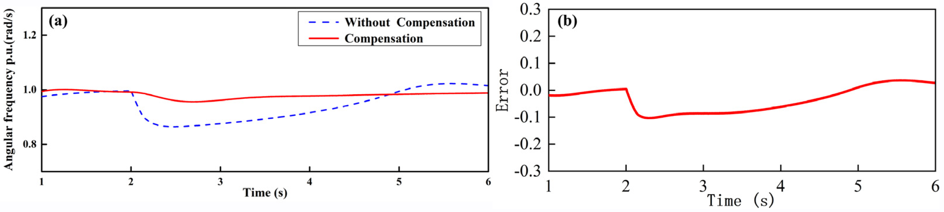
Figure 3 shows the frequency response of the power generation system with and without the compensation system. The natural gas generator system was an impulse by a 400 kW resistive load at the 2 s moment. As can be seen in Figure 3, the compensation system makes the frequency overshoot of the generator set smaller under the impact load. However, the compensation system also imposes a long setting time for the generator. Because (21) and (22) construct feedback linearized controllers to satisfy the system’s asymptotic stability but leave the system with a contradiction between overshoot and setting time. Note that if the controller can ensure the frequency deviation is within the allowable range, the longer the settling time of the generator is instead beneficial to the stability of the system. In a real system, the rotational inertia of a high-power motor is large. This character takes a longer settling time to make the generator transition from one steady state to another.
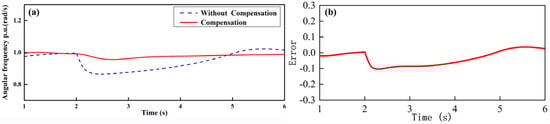
Figure 3.
Bus frequency waveform with and without compensation system (a) frequency waveform, (b) Waveform of error in frequency.
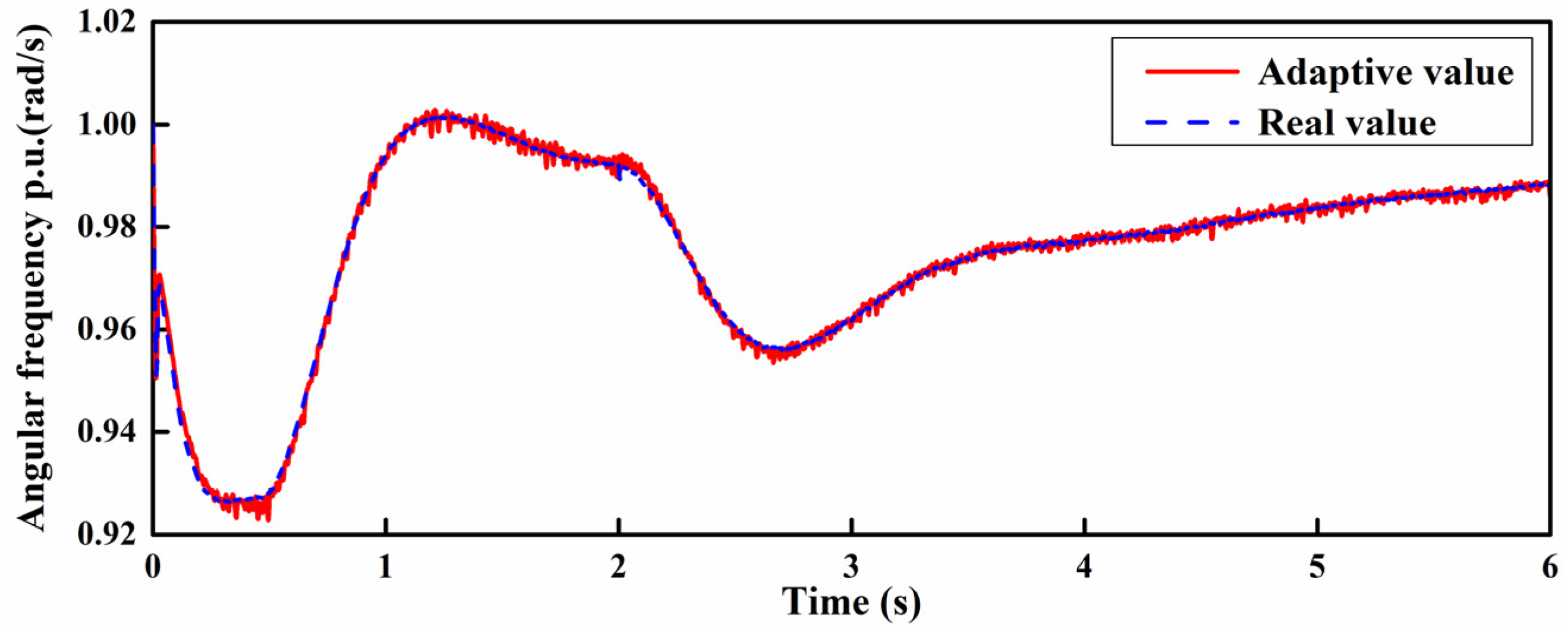
Figure 4 shows the angular frequency waveform controlled by the adaptive algorithm. Comparing Equations (37) and (29), it can be found that the angular frequency is not included in Equation (37), and it can be proved that the active and reactive power outputs of the compensated system converge to the desired values in a finite time according to Lyapunov theory. It is exactly because the stability Equation (37) does not ultimately contain the angular frequency; the angular frequency is theoretically only bounded by stablity. Figure 4 serves as a simulation result, and although the figure achieves a steady state error equal to zero for the angular frequency, the asymptotic stability as a subset of the bounded stability makes this phenomenon not contradictory to the theoretical analysis.
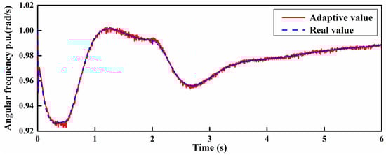
Figure 4.
Angular frequency adaptive algorithm response waveform.
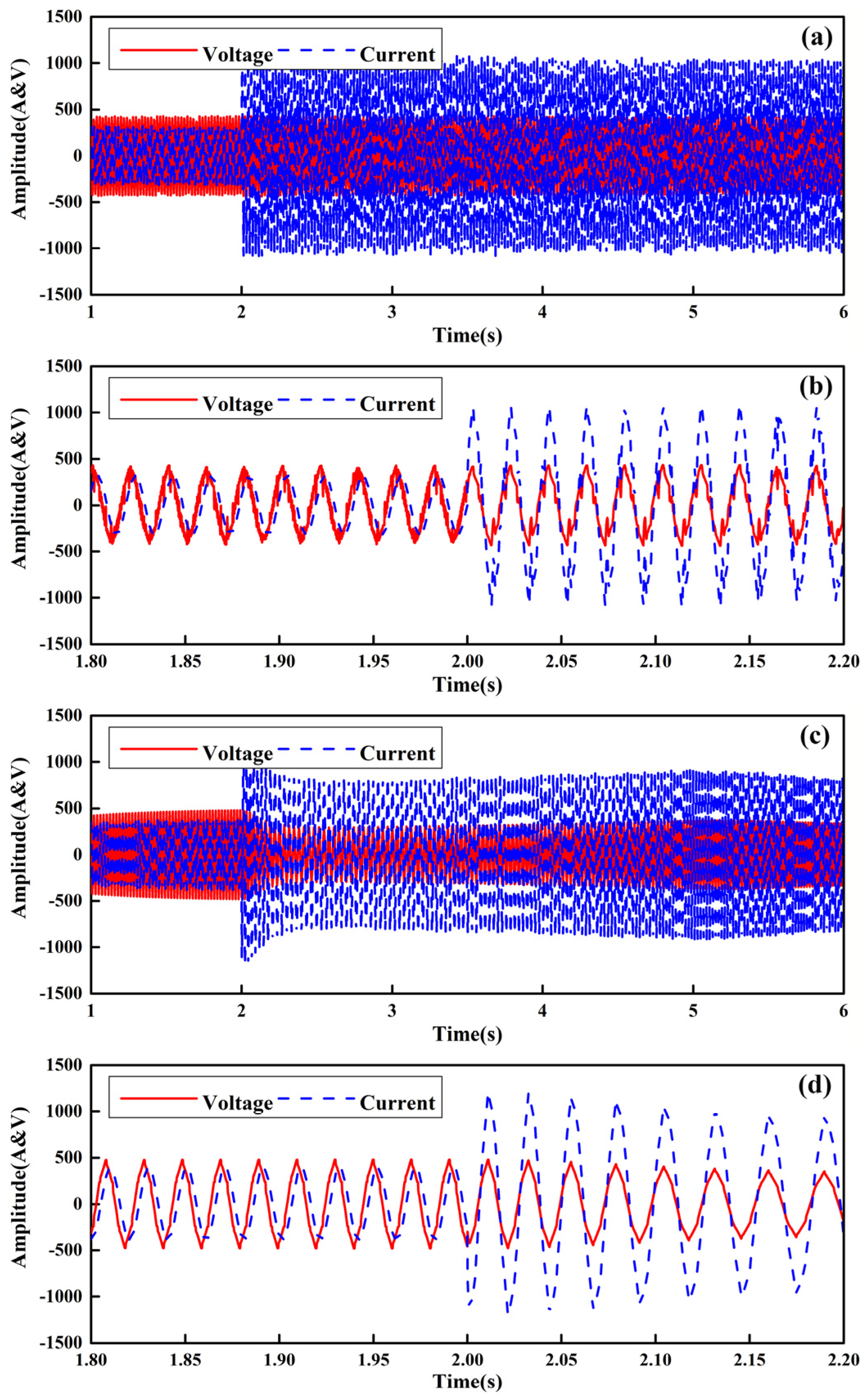
Figure 5 shows the load voltage and current waveforms. Figure 5a,b are waveforms with the compensation system, and Figure 5c,d are the load voltage and current waveforms without the compensation system. Comparing Figure 5b,d, we can see that the system is in a steady state until two seconds, and the rectifier and reactive loads present in the system make the waveform have some degree of phase difference. However, the waveform in Figure 5b shows a larger waveform distortion compared with (d) when the time is equal to 2 s. This means that the output power of the generator is jittering at this moment. This is harmful for high-power generators, and it can even cause shaft excitation problems and damage the rotor shaft. In comparison with 5a,c, the current waveform of the (b) only shows a step at 2 s and no jitter after 2 s. This phenomenon means that the impact load achieves power balance in a short period of time. Note that this generator is unable to provide enough impact power at this moment. As a result, the majority of power is provided by the compensation system.
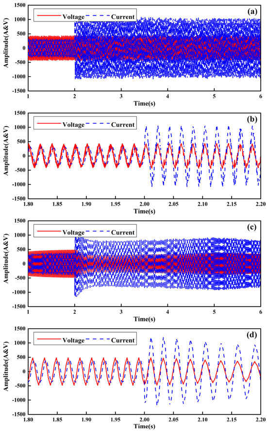
Figure 5.
Voltage and current waveform of the load (a) With compensation system, (b) Moment of loading with compensation system, (c) Without compensation system, (d) Moment of loading without compensation system.
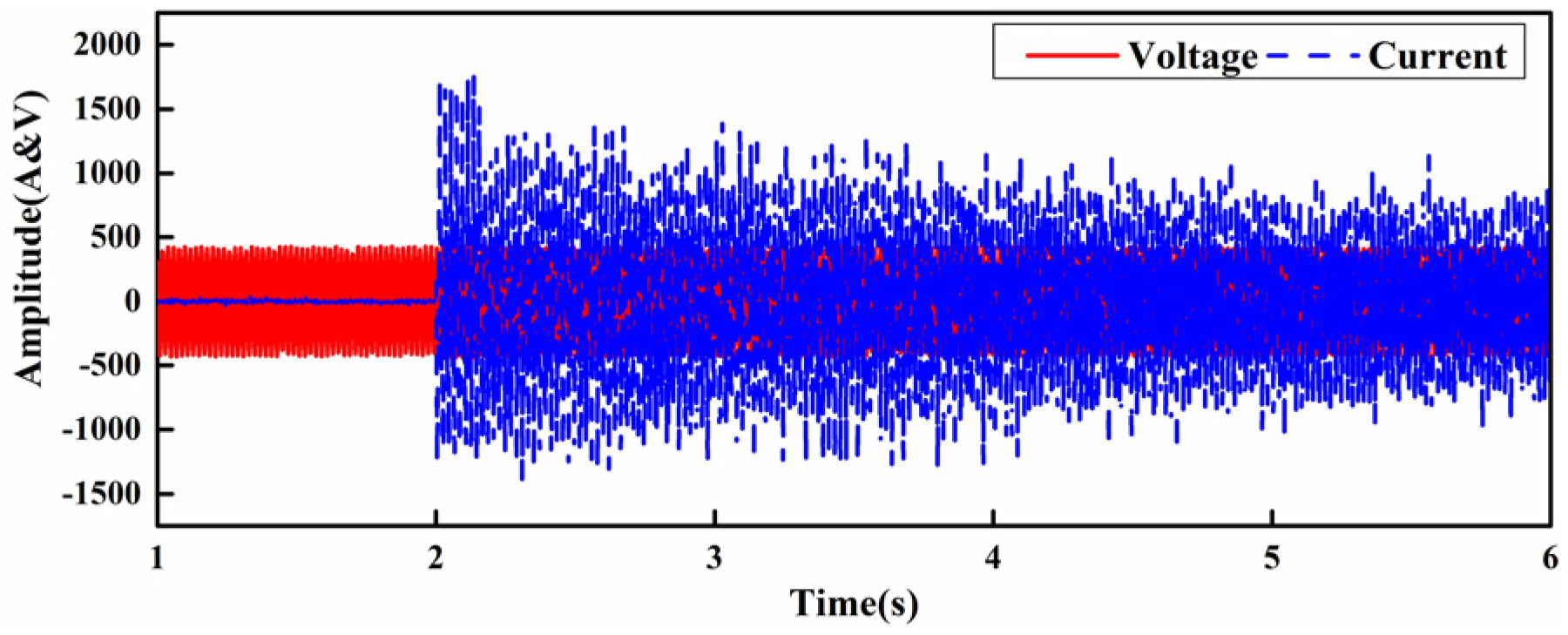
Figure 6 shows the voltage and current waveforms of the output of the compensation system. Figure 6 shows that the compensation system is in a steady state until 2 s. In this interval, the output power of the compensation system is approximately equal to zero. This is due to the reference values for both active and reactive power being set to zero in (16). For compensated systems, the impact load becomes a disturbance term to test the robustness of the adaptive controller. Because the purpose of the compensation system is to help the generator through the speed regulation period, the compensation system will exit the dynamic regulation process when the generator speed returns to the rated speed. After the compensation process, the inverter output active and reactive power is equal to zero when the generator returns to a steady state. This idea of treating impact load as a dynamic disturbance achieves a fast response of the load power.
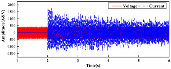
Figure 6.
Compensation system voltage and current waveform.
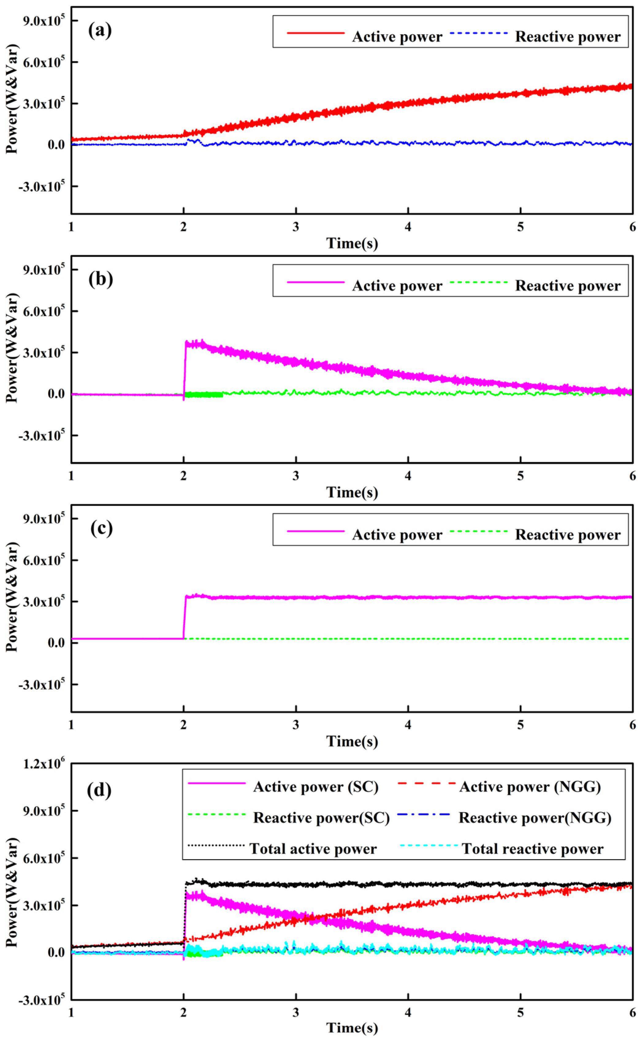
Figure 7a–c shows the power response waveforms of the generator, the compensation system, and the load, respectively. Comparing Figure 7a,b, the compensated system output power before 2 s is equal to zero when the system is in a steady state. The output power of the generator is equal to the line impedance and the no-load loss. When time is equal to 2 s, Figure 7a shows a smooth and slow rise in the output power of the generator, and Figure 7b shows a surge in the output power of the compensation system. This phenomenon means that the compensation system achieves high power discharge in an instant. This result also reveals the selection of super capacitor as the energy source of the compensation system in this paper. Meanwhile, combined with Figure 7a,b, it can be seen that compensation power comes from two components in this instantaneous, and Figure 7b shows that the most important is from the compensation system. When time is equal to 5 s, Figure 7a,b indicates that the compensation system is gradually withdrawing from the compensation process. The compensation system is fully withdrawn until the engine reaches rated speed. Figure 7a–c demonstrates that the proposed NAMIMO controller effectively achieves the compensation of impact load. Figure 7d shows the power waveform of the compensation and the natural gas generation system. Figure 7d shows that the compensation system allows the impact load to achieve power balance. Note that although the impact load is active power, there is also a brief fluctuation in reactive power. Equation (7) explains active and reactive power are coupled in the compensation system. This also displays that direct power control is closer to the nature of the whole system.
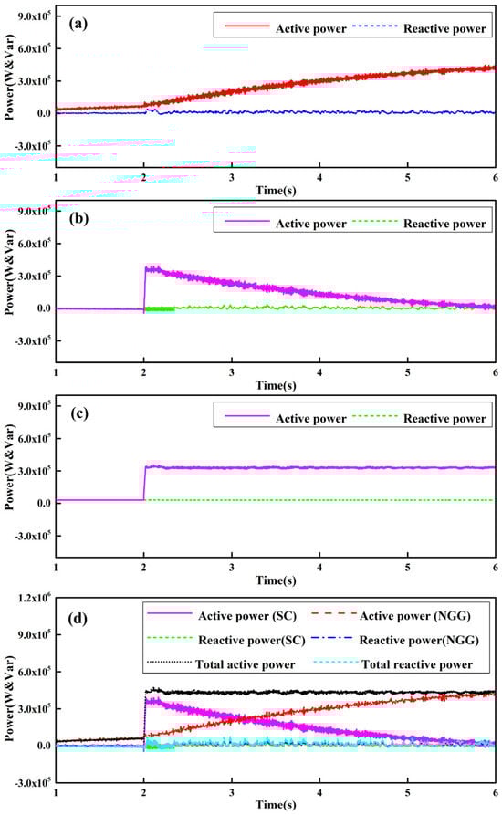
Figure 7.
The waveform of power response (a) Power response of generator, (b) Power response of compensation system, (c) Power response of impact load, (d) Response summary.
4.2. Experiment Analysis of the Compensation System Response
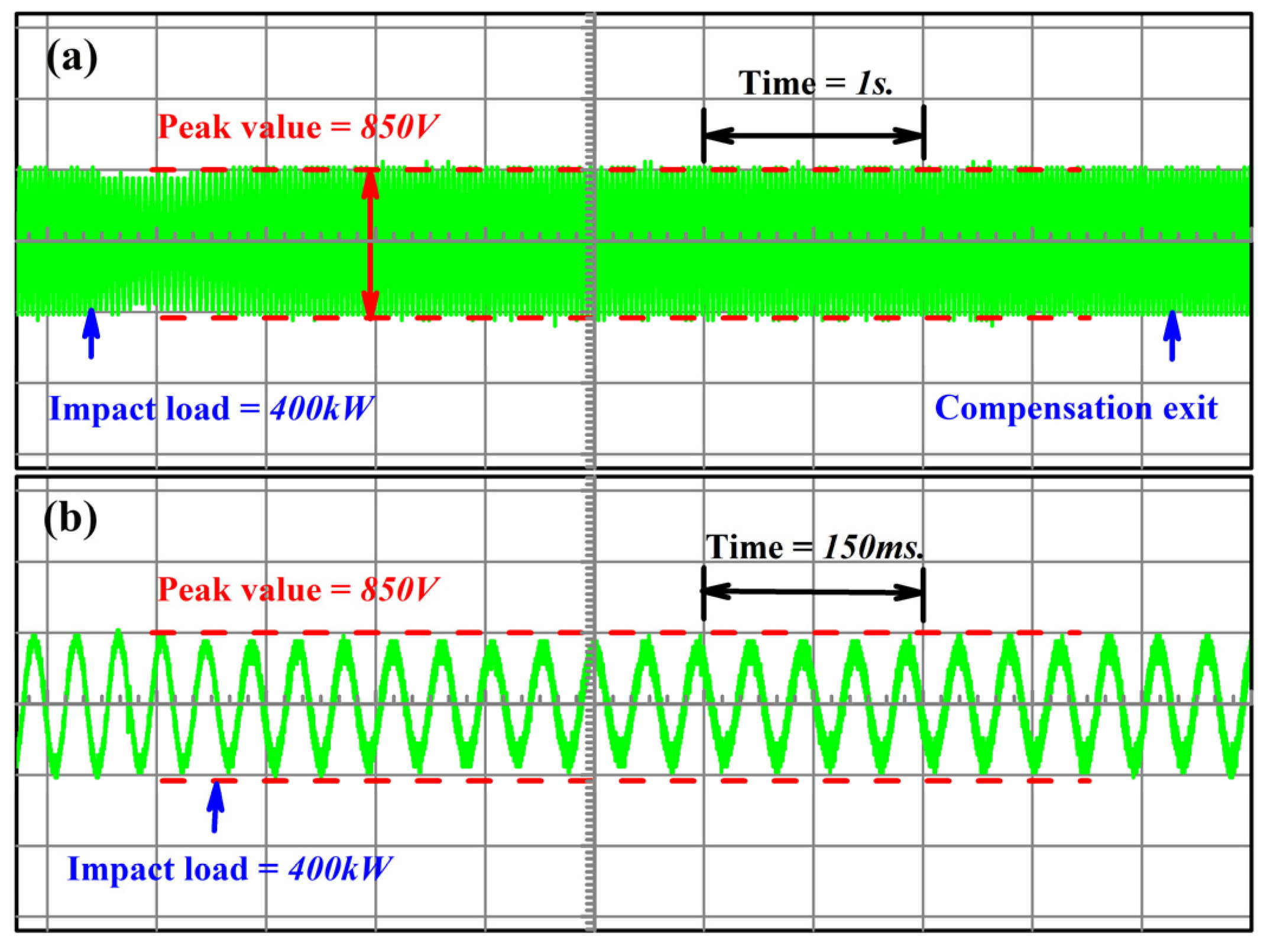
Figure 8 shows the DC bus voltage response waveform of the compensation system. The figure shows that the bus voltage is kept at 785 V when the system is in a steady state. In other words, the compensation system is not working at this moment. The voltage at the bus starts to rise sharply when the system is subjected to the 400 kW impact load. This process indicates that the super capacitor is discharging outward through the DC/DC converter. Due to the virtual inertia of a super capacitor being much smaller than the natural gas generator, super capacitors can discharge a large amount of energy in a very short period of time. After about 4 s, the natural gas generator speed increases to the rated speed, and the compensation system gradually exits the compensation process. At this time, although the output current of the compensation system can be turned off directly by the IGBT, the voltage out of the bus still drops slowly due to the existence of inertia.
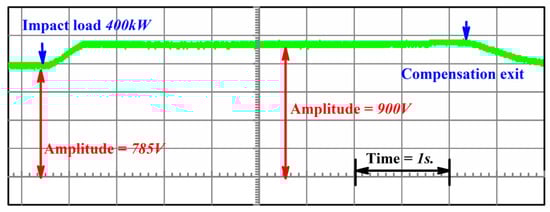
Figure 8.
The waveform of DC bus voltage.
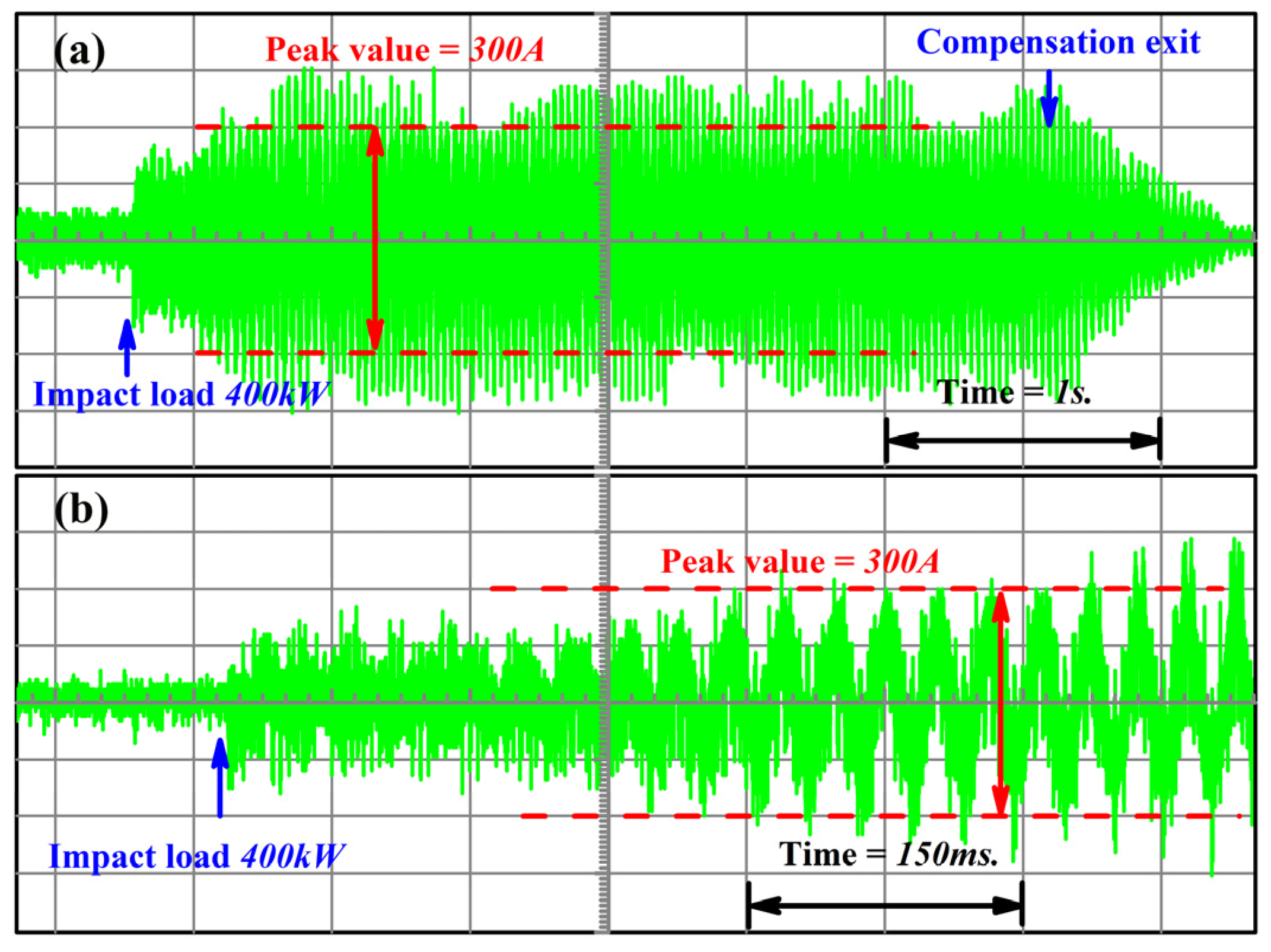
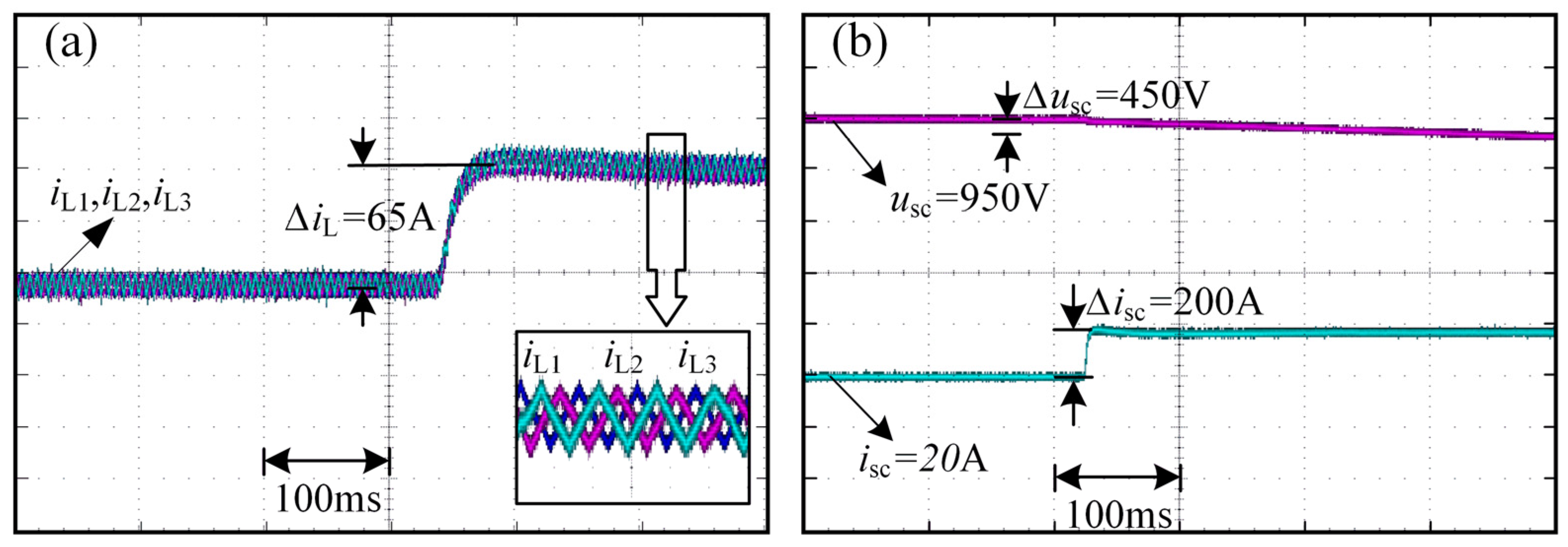
Figure 9 shows the voltage and current waveform at the AC-bus (#PCC). Figure 10 shows the voltage and current waveform of the DC bus. From Figure 9a,b, it can be seen that the voltage of the AC-bus does not change before and after suffering the impact load. This is due to the presence of the excitation system, which keeps the generator output voltage essentially constant. From Figure 10a,b, it can be seen that the current on the AC-bus rises sharply with the presence of the impact load. Meanwhile, as can be clearly seen in Figure 10b, the bus current rises to a maximum value in a very short period of time and remains constant. Note that although the current shows a rapid upward trend, there are large harmonics in the graph. This is due to the fact that the proposed control strategy uses direct power control, which ensures the fast response characteristics of the power but makes the harmonic content of the current larger. Of course, natural gas generators cannot provide so much power to bear the impact load in this short period of time. The trend of the whole impact load power and the current are basically the same when the bus voltage is constant. This conclusion has a good match with the simulation Figure 7c. Figure 11. Generator transient response during impact load loading and its phenomena are in agreement with Figure 9 and Figure 10. Figure 12 shows the inductor current waveforms of the triple staggered parallel DC/DC converter of the compensation system. From the figure, it can be seen that the triple currents differ from each other by 120°. The independent current PI controller not only makes the compensation device have better current equalization characteristics, but also the total current ripple is well improved, effectively reducing the total current ripple amount. As a result, the system reliability is significantly improved.
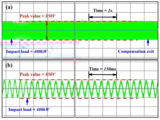
Figure 9.
The waveform of AC bus voltage (a) Whole time, (b) Loading moment.
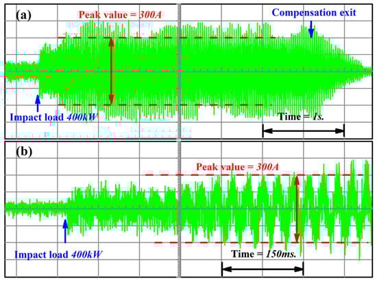
Figure 10.
The waveform of AC current (a) Whole time, (b) Loading moment.
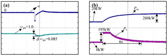
Figure 11.
Generator transient response during impact load loading (a) Angular frequency and acceleration, (b) Electromagnetic and mechanical power.

Figure 12.
Compensation system transient response during impact load loading (a) Inductor currents, (b) Supercapacitor Current and Voltage.
In a word, the super capacitor compensation system can effectively improve the load characteristics of natural gas generators, especially in the face of rough operating conditions such as impact loads. Finally, the experimental results in Figure 9 and Figure 10 show that the experiments and simulations have the same results. However, it should be added that although this paper has achieved the realization of power compensation in the proposed microgrid. However, compared with the literature [24,25,26], the proposed control strategy is not able to achieve inertia response and voltage support in the grid. On the contrary, the proposed control strategy has the advantage of maintaining a fast power balance after the microgrid is connected to the impact load compared with the above references. In addition, the strategy has the same disadvantage as the literature [29,30], i.e., large current harmonics.
5. Conclusions
In this paper, a super capacitor compensation device is added to the natural generator system, and a NAMIMO controller is proposed to control the compensation device. The proposed strategy and algorithm can effectively improve the load characteristics of the natural gas generator. Compared with a power generation system without compensation devices, the latter can not only effectively reduce the effect of impact loads on the generator, but also make the generator have a fast frequency response.
First, this paper establishes a mathematical model of the microgrid, which describes the transient response of the output power of the compensation device and the generator set. Second, based on the established model, the NAMIMO control algorithm is designed to realize the fast-tracking control of the frequency of the compensation device. A control group is designed to compare the proposed control algorithm to demonstrate the response of the proposed control algorithm in the face of shock loads to ensure the stability of the system. Finally, a dual-generator microgrid with a capacity of 600 kW is established, and the effectiveness of the proposed control strategy is verified on the constructed platform.
Overall, simulation and experimental results prove that the proposed compensation structure can effectively help natural gas generators reduce the effect of the impact load. However, with a large number of electronic devices connected to the microgrid the loads are nonlinear. How to solve the harmonic problem becomes further research in this article. In addition, this article has only been investigated for impact loads, and the performance of the compensation strategy regarding pulse load conditions will be verified in future work.
Author Contributions
S.W. proposed the idea, conducted the experimental validation, and completed the manuscript writing; K.Z. provided experiment equipment; J.D. improved the experimental scheme and funded the research; J.D. edited the software procedure; L.S. coordinated the resources and reviewed the manuscript. All authors have read and agreed to the published version of the manuscript.
Funding
This research is funded by the National Natural Science Foundation of China (grant number 52177211) and by the Heilongjiang Postdoctoral Research Starting Fund (grant number LBH-Q20020).
Institutional Review Board Statement
Not applicable.
Informed Consent Statement
Not applicable.
Data Availability Statement
The original contributions presented in the study are included in the article, further inquiries can be directed to the corresponding author.
Acknowledgments
We thank Ding for his suggestions regarding the experimental scheme of this paper.
Conflicts of Interest
The authors declare no conflicts of interest.
References
- Odetayo, B.; Kazemi, M.; MacCormack, J. A Chance Constrained Programming Approach to the Integrated Planning of Electric Power Generation, Natural Gas Network and Storage. IEEE Trans. Smart Grid. 2018, 33, 6883–6893. [Google Scholar] [CrossRef]
- Xiao, J.; Bai, L.; Li, F. Sizing of Energy Storage and Diesel Generators in an Isolated Microgrid Using Discrete Fourier Transform (DFT). IEEE Trans. Sustain. Energy 2014, 5, 907–916. [Google Scholar] [CrossRef]
- Li, Y.; Fan, L.; Miao, Z. Wind in Weak Grids: Low-Frequency Oscillations, Subsynchronous Oscillations, and Torsional Interactions. IEEE Trans. Power Syst. 2020, 35, 109–117. [Google Scholar] [CrossRef]
- Zhao, Y.Y.; Guo, H.; Wang, L.K. Computer Modeling of the Eddy Current Losses of Metal Fasteners in Rotor Slots of a Large Nuclear Steam Turbine Generator Based on Finite-Element Method and Deep Gaussian Process Regression. IEEE Trans. Ind. Electron. 2020, 67, 5349–5359. [Google Scholar] [CrossRef]
- Bellache, K.; Camara, M.B.; Dakyo, B. Transient Power Control for Diesel-Generator Assistance in Electric Boat Applications Using Supercapacitors and Batteries. IEEE J. Emerg. Sel. Top. Power Electron. 2018, 6, 416–428. [Google Scholar] [CrossRef]
- Li, M.; Wang, L.; Wang, Y.J. Sizing Optimization and Energy Management Strategy for Hybrid Energy Storage System Using Multiobjective Optimization and Random Forests. IEEE Trans. Power Electron. 2021, 36, 11421–11430. [Google Scholar] [CrossRef]
- Zhou, S.Y.; Chen, Z.Q.; Huang, D.Y. Model Prediction and Rule Based Energy Management Strategy for a Plug-in Hybrid Electric Vehicle with Hybrid Energy Storage System. IEEE Trans. Power Electron. 2021, 36, 5926–5940. [Google Scholar] [CrossRef]
- Ahn, J.-H.; Lee, B.K. High-Efficiency Adaptive-Current Charging Strategy for Electric Vehicles Considering Variation of Internal Resistance of Lithium-Ion Battery. IEEE Trans. Power Electron. 2019, 34, 3041–3052. [Google Scholar] [CrossRef]
- Kotra, S.; Mishra, M.K. Design and Stability Analysis of DC Microgrid with Hybrid Energy Storage System. IEEE Trans. Sustain. Energy. 2019, 10, 1603–1610. [Google Scholar] [CrossRef]
- Zhang, Q.; Li, G. Experimental Study on a Semi-Active Battery-Supercapacitor Hybrid Energy Storage System for Electric Vehicle Application. IEEE Trans. Power Electron. 2020, 35, 1014–1021. [Google Scholar] [CrossRef]
- Hou, J.; Song, Z.; Hofmann, H.F. Control Strategy for Battery/Flywheel Hybrid Energy Storage in Electric Shipboard Microgrids. IEEE Trans. Ind. Inform. 2021, 17, 1089–1099. [Google Scholar] [CrossRef]
- Charalambous, A.; Hadjidemetriou, L.; Kyriakides, E. A Coordinated Voltage–Frequency Support Scheme for Storage Systems Connected to Distribution Grids. IEEE Trans. Power Electron. 2021, 36, 8464–8475. [Google Scholar] [CrossRef]
- Oskouee, S.S.; Kamali, S.; Amraee, T. Primary Frequency Support in Unit Commitment Using a Multi-Area Frequency Model with Flywheel Energy Storage. IEEE Trans. Power Syst. 2021, 36, 5105–5119. [Google Scholar] [CrossRef]
- Nguyen, T.; Yoo, H.; Kim, H. Applying Model Predictive Control to SMES System in Microgrids for Eddy Current Losses Reduction. IEEE Trans. Appl. Supercond. 2016, 25, 5400405. [Google Scholar] [CrossRef]
- Xu, Y.; Li, Y.; Ren, L.; Xu, C.; Tang, Y.; Li, J.; Chen, L.; Jia, B. Research on the Application of Superconducting Magnetic Energy Storage in Microgrids for Smoothing Power Fluctuation Caused by Operation Mode Switching. IEEE Trans. Appl. Supercond. 2018, 28, 5701306. [Google Scholar] [CrossRef]
- Liu, K.; Zhu, C.; Lu, R.; Chan, C.C. Improved Study of Temperature Dependence Equivalent Circuit Model for Supercapacitors. IEEE Trans. Plasma Sci. 2013, 41, 1267–1271. [Google Scholar]
- Zhu, D.; Zhou, S.; Zou, X. Improved Design of PLL Controller for LCL-Type Grid-Connected Converter in Weak Grid. IEEE Trans. Power Electron. 2020, 35, 4715–4727. [Google Scholar] [CrossRef]
- Guo, X.; Guerrero, J.M.; Wu, B. Space Vector Modulation for DC-Link Current Ripple Reduction in Back-to-Back Current-Source Converters for Microgrid Applications. IEEE Trans. Ind. Electron. 2015, 62, 6008–6013. [Google Scholar] [CrossRef]
- Bouafia, A.; Gaubert, J.; Krim, F. Predictive Direct Power Control of Three-Phase Pulsewidth Modulation (PWM) Rectifier Using Space-Vector Modulation (SVM). IEEE Trans. Power Electron. 2010, 25, 228–236. [Google Scholar] [CrossRef]
- Meng, X.; Liu, J.; Liu, Z. A Generalized Droop Control for Grid-Supporting Inverter Based on Comparison Between Traditional Droop Control and Virtual Synchronous Generator Control. IEEE Trans. Power Electron. 2019, 34, 5416–5438. [Google Scholar] [CrossRef]
- Dong, D.; Wen, B.; Boroyevich, D.; Mattavelli, P.; Xue, Y. Analysis of Phase-Locked Loop Low-Frequency Stability in Three-Phase Grid-Connected Power Converters Considering Impedance Interactions. IEEE Trans. Ind. Electron. 2015, 62, 310–321. [Google Scholar] [CrossRef]
- Silwal, S.; Taghizadeh, S.; Karimi-Ghartemani, M.; Hossain, M.J. An Enhanced Control System for Single-Phase Inverters Interfaced with Weak and Distorted Grids. IEEE Trans. Power Electron. 2019, 34, 12538–12551. [Google Scholar] [CrossRef]
- Wang, X.; Harnefors, L.; Blaabjerg, F. Unified Impedance Model of Grid-Connected Voltage-Source Converters. IEEE Trans. Power Electron. 2018, 32, 1775–1787. [Google Scholar] [CrossRef]
- Chen, S.; Sun, Y.; Hou, X.; Han, H. Quantitative Parameters Design of VSG Oriented to Transient Synchronization Stability. IEEE Trans. Power Syst. 2019, 38, 4978–4981. [Google Scholar] [CrossRef]
- Koiwa, K.; Inoo, K.; Zanma, T.; Liu, K.-Z. Virtual Voltage Control of VSG for Overcurrent Suppression Under Symmetrical and Asymmetrical Voltage Dips. IEEE Trans. Ind. Electron. 2022, 69, 11177–11186. [Google Scholar] [CrossRef]
- Li, G.; Song, W.; Liu, X. A Quasi-Harmonic Voltage Feedforward Control for Improving Power Quality in VSG-Based Islanded Microgrid. IEEE J. Emerg. Sel. Topics Power Electron. 2024, 12, 2994–3004. [Google Scholar] [CrossRef]
- Gui, Y.; Wang, X.; Blaabjerg, F. Vector Current Control Derived from Direct Power Control for Grid-Connected Inverters. IEEE Trans. Power Electron. 2019, 34, 9224–9235. [Google Scholar] [CrossRef]
- Zhang, Y.; Jiao, J.; Liu, J.; Gao, J. Direct Power Control of PWM Rectifier with Feedforward Compensation of DC-Bus Voltage Ripple Under Unbalanced Grid Conditions. IEEE Trans. Ind. Appl. 2019, 55, 2890–2901. [Google Scholar] [CrossRef]
- Zhang, Y.; Jiao, J.; Liu, J. Direct Power Control of PWM Rectifiers with Online Inductance Identification Under Unbalanced and Distorted Network Conditions. IEEE Trans. Power Electron. 2019, 34, 12524–12537. [Google Scholar] [CrossRef]
- Sato, A.; Noguchi, T. Voltage-Source PWM Rectifier–Inverter Based on Direct Power Control and Its Operation Characteristics. IEEE Trans. Power Electron. 2011, 26, 1559–1567. [Google Scholar] [CrossRef]
- Kelly, R.; Santibanez, V.; Loria, A. Control of Robot Manipulators in Joint Space; Springer: Berlin/Heidelberg, Germany, 2005; pp. 392–394. [Google Scholar]


Disclaimer/Publisher’s Note: The statements, opinions and data contained in all publications are solely those of the individual author(s) and contributor(s) and not of MDPI and/or the editor(s). MDPI and/or the editor(s) disclaim responsibility for any injury to people or property resulting from any ideas, methods, instructions or products referred to in the content. |
© 2025 by the authors. Licensee MDPI, Basel, Switzerland. This article is an open access article distributed under the terms and conditions of the Creative Commons Attribution (CC BY) license (https://creativecommons.org/licenses/by/4.0/).