
Towards an Automatic Recognition of Artifacts and Features in Plethysmographic Traces

 , , , , , , and
Abstract
:1. Introduction
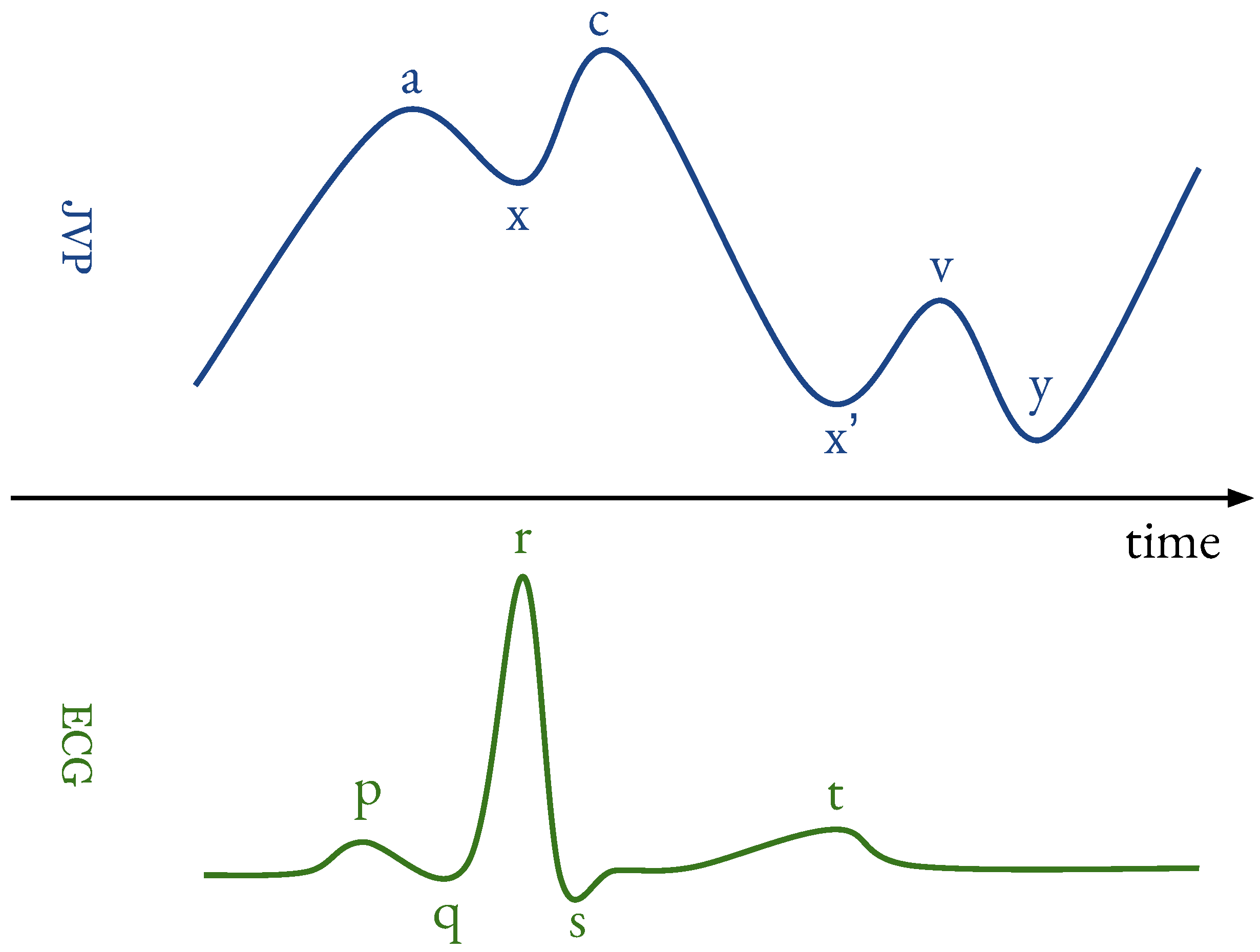
- a
- : originates from active atrial contraction leading to retrograde blood flow into neck veins.
- x
- : caused by continued atrial relaxation.
- c
- : due to the impact of the carotid artery adjacent to the jugular vein and retrograde transmission of a positive wave in the right atrium, produced by the right ventricular systole and the bulging of the tricuspid valve into the right atrium.
- : caused by the descent of the right atrium floor (tricuspid valve) during right ventricular systole and continued atrial relaxation.
- v
- : corresponds to the maximal atrial filling; it is less prominent than the a ascent wave.
- y
- : follows the v wave and corresponds to the emptying of the atrium.
2. Related Works
3. Data Collection and Preparation
3.1. A Summary of the Capacitive Strain-Gauge Sensor and Experimental Activity
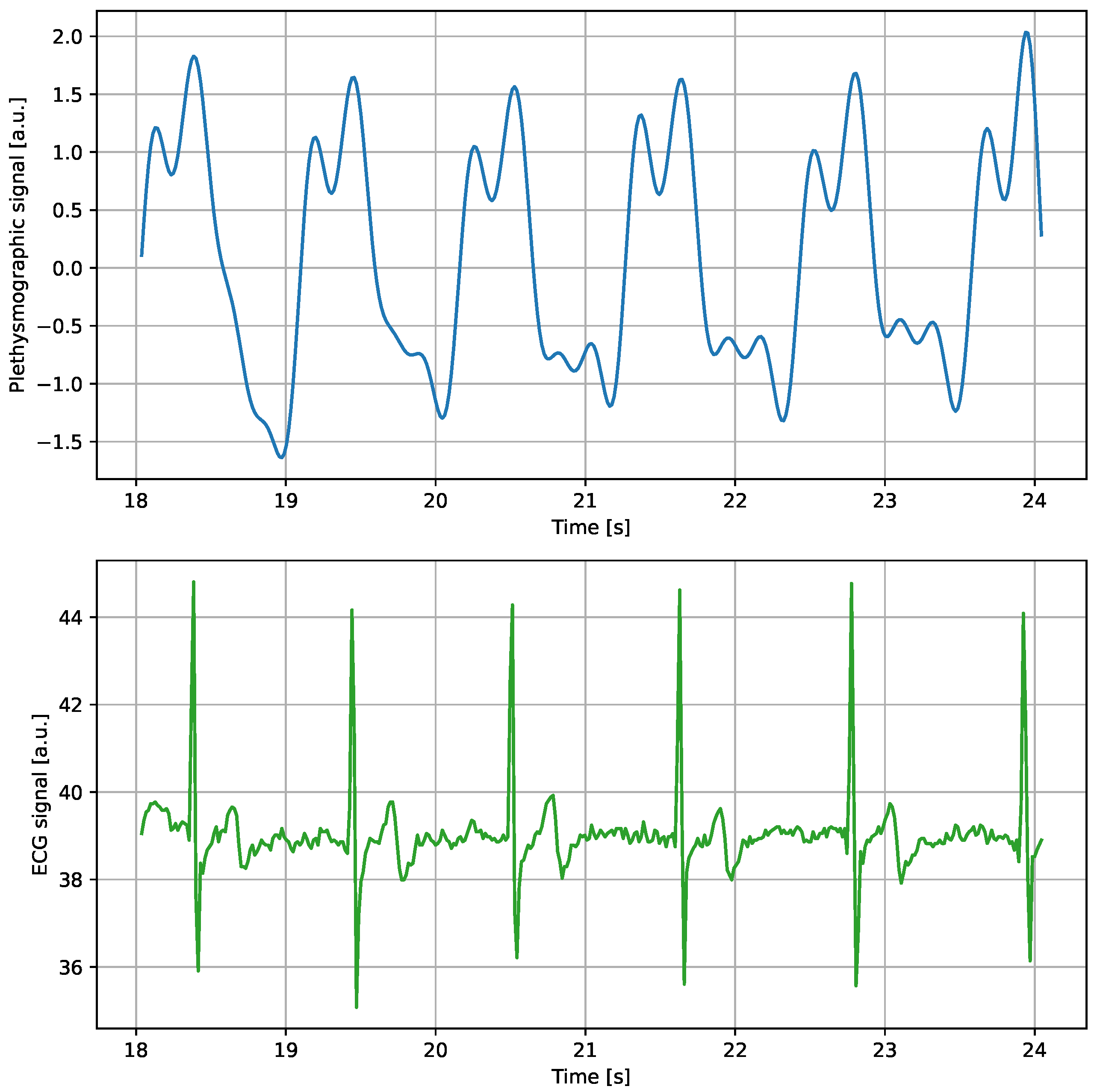
3.2. Data Collection
3.3. Annotations
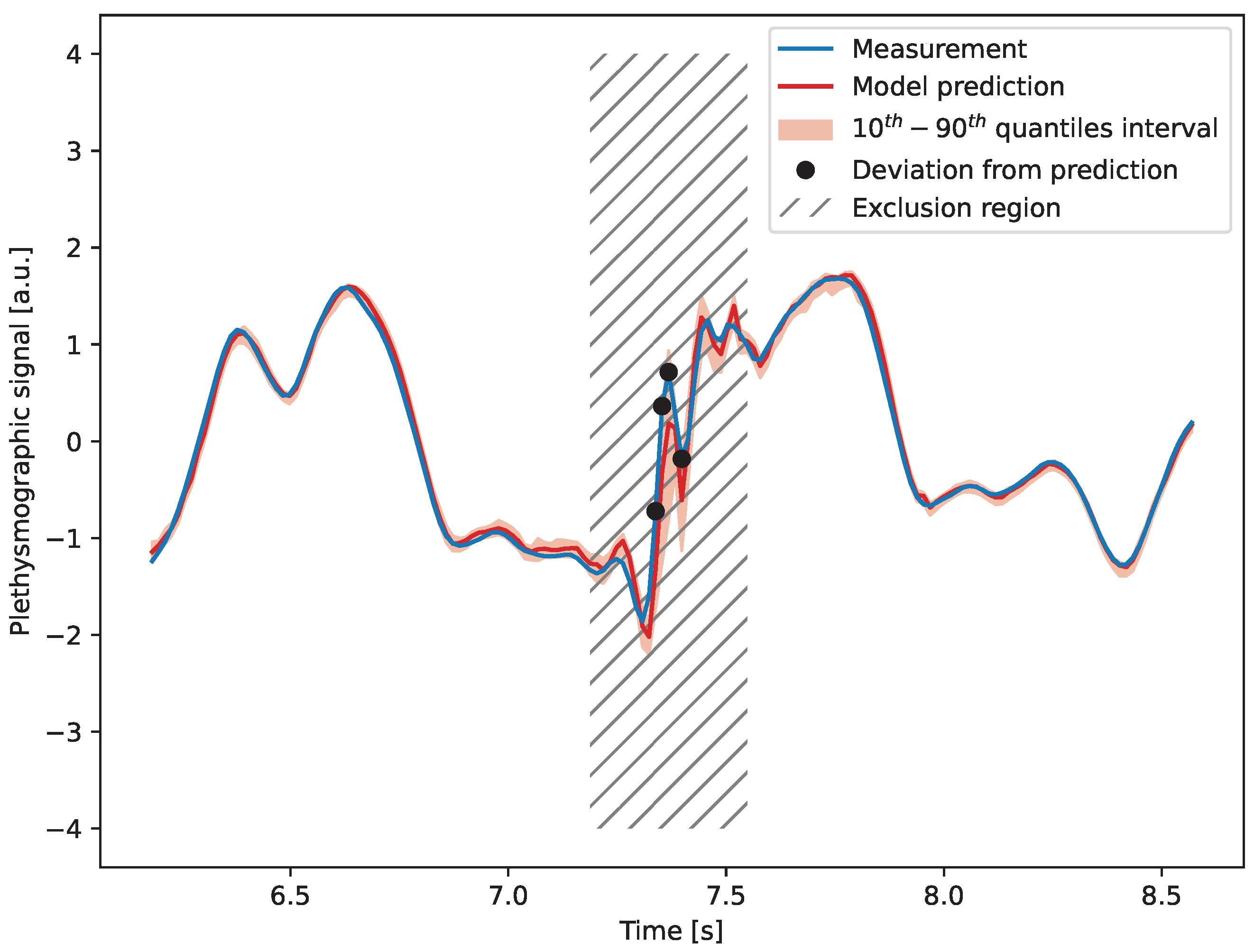
4. Detection of Artifacts
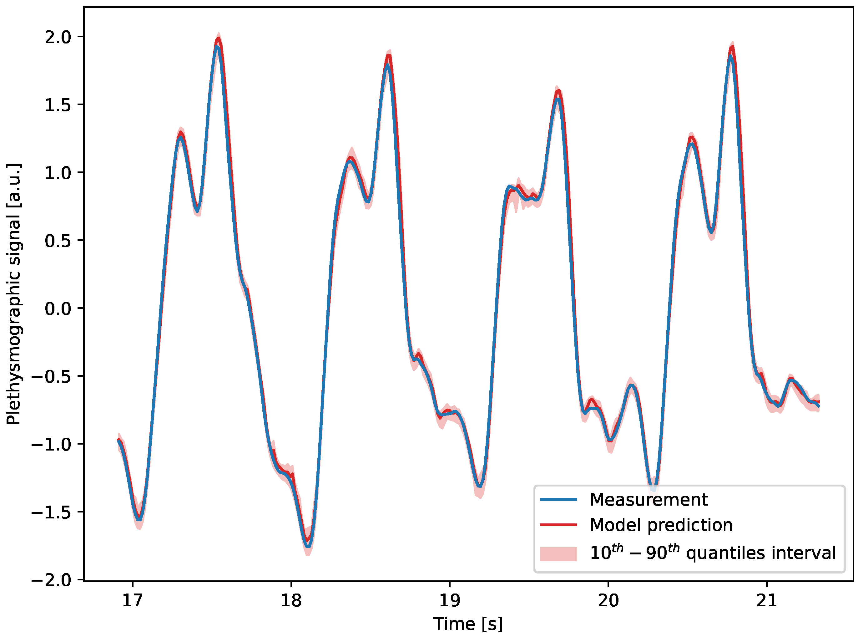
4.1. Model Description
4.2. Results
5. Feature Identification
5.1. Model Description
5.2. Results
6. Conclusions
Author Contributions
Funding
Institutional Review Board Statement
Informed Consent Statement
Data Availability Statement
Acknowledgments
Conflicts of Interest
References
- Scerrati, A.; Menegatti, E.; Zamboni, M.; Malagoni, A.M.; Tessari, M.; Galeotti, R.; Zamboni, P. Internal Jugular Vein Thrombosis: Etiology, Symptomatology, Diagnosis and Current Treatment. Diagnostics 2021, 11, 378. [Google Scholar] [CrossRef]
- Zamboni, P.; Malagoni, A.M.; Menegatti, E.; Ragazzi, R.; Tavoni, V.; Tessari, M.; Beggs, C.B. Central venous pressure estimation from ultrasound assessment of the jugular venous pulse. PLoS ONE 2020, 15, e0240057. [Google Scholar] [CrossRef] [PubMed]
- Menegatti, E.; Proto, A.; Paternò, G.; Gadda, G.; Gianesini, S.; Raisi, A.; Pagani, A.; Piva, T.; Zerbini, V.; Mazzoni, G.; et al. The Effect of Submaximal Exercise on Jugular Venous Pulse Assessed by a Wearable Cervical Plethysmography System. Diagnostics 2022, 12, 2407. [Google Scholar] [CrossRef]
- Proto, A.; Conti, D.; Menegatti, E.; Taibi, A.; Gadda, G. Plethysmography System to Monitor the Jugular Venous Pulse: A Feasibility Study. Diagnostics 2021, 11, 2390. [Google Scholar] [CrossRef] [PubMed]
- Cretescu, I.; Horhat, R.; Mocanu, V.; Munteanu, O. Bioelectrical Impedance Versus Air-Displacement Plethysmography for Body Fat Measurements in Subjects with Abdominal Obesity: A Comparative Study. Appl. Sci. 2025, 15, 2056. [Google Scholar] [CrossRef]
- Soggia, B.; Pagani, A.; Proto, A.; Brancaccio, R.; Taibi, A. Extraction of the Jugular Venous Pulse and carotid profile using a cervical contact plethysmography system. Veins Lymphat. 2024, 13, 12664. [Google Scholar] [CrossRef]
- Lambert Cause, J.; Solé Morillo, Á.; García-Naranjo, J.C.; Stiens, J.; da Silva, B. The Impact of Contact Force on Signal Quality Indices in Photoplethysmography Measurements. Appl. Sci. 2024, 14, 5704. [Google Scholar] [CrossRef]
- Menegatti, E.; Proto, A.; Paternò, G.; Gianesini, S.; Pagani, A.; Tommaso, P.; Andrea, R.; Zerbini, V.; Taibi, A.; Zamboni, P.; et al. Assessment of jugular venous pulse during walking by wearable strain-gauge plethysmograph: A pilot study. In Proceedings of the 2022 IEEE International Workshop on Sport, Technology and Research (STAR), Cavalese, Italy, 13–15 July 2022; pp. 51–55. [Google Scholar] [CrossRef]
- Werner, J.D.; Siskin, G.P.; Mandato, K.; Englander, M.; Herr, A. Review of Venous Anatomy for Venographic Interpretation in Chronic Cerebrospinal Venous Insufficiency. J. Vasc. Interv. Radiol. 2011, 22, 1681–1690. [Google Scholar] [CrossRef]
- Mari, S.; Pagani, A.; Valentini, G.; Mascetti, G.; Pignataro, S.; Proto, A.; Menegatti, E.; Taibi, A.; Zamboni, P. Monitoring the cerebral venous drainage in space missions: The Drain Brain experiments of the Italian Space Agency. Veins Lymphat. 2023, 12, 11716. [Google Scholar] [CrossRef]
- Nguyen, T.; Dinh, A.; Bui, F.M.; Vo, T. A Novel Non-invasive System for Acquiring Jugular Venous Pulse Waveforms. In 5th International Conference on Biomedical Engineering in Vietnam; Toi, V.V., Lien Phuong, T.H., Eds.; Springer: Cham, Switzerland, 2015; pp. 75–78. [Google Scholar]
- George, N.R.; Girish, V.V.; Jaganathan, G.; Kiran V, R.; Nabeel, P.M.; Sivaprakasam, M.; Joseph, J. Wearable Accelerometer System for Jugular Venous Pulse Quantification: A Pilot Study. In Proceedings of the 2024 IEEE International Symposium on Medical Measurements and Applications (MeMeA), Eindhoven, The Netherlands, 26–28 June 2024; pp. 1–5. [Google Scholar] [CrossRef]
- Karhinoja, K.; Sirkiä, J.P.; Panula, T.; Kaisti, M.; Koivisto, T.; Pänkäälä, M. Method for measuring jugular venous pulse with a miniature gyroscope sensor patch. In Proceedings of the 2023 45th Annual International Conference of the IEEE Engineering in Medicine and Biology Society (EMBC), Sydney, Australia, 24–27 July 2023; pp. 1–4. [Google Scholar] [CrossRef]
- George, N.R.; Sudarsan, N.; Manoj, R.; Kiran V, R.; Nabeel, P.M.; Sivaprakasam, M.; Joseph, J. Jugular Venous Pulse Waveform Acquisition using Contact Piezo Sensor: A Pilot Study. In Proceedings of the 2024 46th Annual International Conference of the IEEE Engineering in Medicine and Biology Society (EMBC), Orlando, FL, USA, 15–19 July 2024; pp. 1–4. [Google Scholar] [CrossRef]
- Singh, R.; Jaffe, A.; Frydman, G.H.; Najia, M.A.T.; Wei, Z.; Yang, J.; Majmudar, M.D. Noninvasive Assessment of Jugular Venous Pressure via Force-Coupled Single Crystal Ultrasound. IEEE Trans. Biomed. Eng. 2018, 65, 1705–1710. [Google Scholar] [CrossRef]
- Hill, J.; Campbell, J.; Chase, J. Estimation of Venous Oxygen Saturation Through Non-Invasive Optical Sensing at the Jugular Veins. Curr. Dir. Biomed. Eng. 2024, 10, 295–298. [Google Scholar] [CrossRef]
- García-López, I.; Rodriguez-Villegas, E. Extracting the Jugular Venous Pulse from Anterior Neck Contact Photoplethysmography. Sci. Rep. 2020, 10, 3466. [Google Scholar] [CrossRef]
- Conroy, T.; Zhou, J.; Kan, E. Jugular Venous Pulse Waveform Extraction From a Wearable Radio Frequency Sensor. IEEE Sens. J. 2023, 23, 10140–10148. [Google Scholar] [CrossRef] [PubMed]
- Das, S.; Dwivedi, G.; Afsharan, H.; Kavehei, O. A Non-Invasive and Non-Contact Jugular Venous Pulse Measurement: A Feasibility Study. medRxiv 2024. [Google Scholar] [CrossRef]
- Suzuki, S.; Hoshiga, M.; Kotani, K.; Asao, T. Assessment of Non-Contact Measurement Using a Microwave Sensor to Jugular Venous Pulse Monitoring. J. Biomed. Sci. Eng. 2021, 14, 94–102. [Google Scholar] [CrossRef]
- Amelard, R.; Hughson, R.; Greaves, D.; Pfisterer, K.; Leung, J.; Clausi, D.; Wong, A. Non-contact hemodynamic imaging reveals the jugular venous pulse waveform. Sci. Rep. 2017, 7, 40150. [Google Scholar] [CrossRef]
- Tang, E.; Hajirassouliha, A.; Nash, M.; Nielsen, P.; Taberner, A.; Cakmak, Y. Non-contact Quantification of Jugular Venous Pulse Waveforms from Skin Displacements. Sci. Rep. 2018, 8, 17236. [Google Scholar] [CrossRef]
- He, Q.; Geng, W.; Li, W.; Wang, R. Non-contact measurement of neck pulses achieved by imaging micro-motions in the neck skin. Biomed. Opt. Express 2023, 14, 4507–4519. [Google Scholar] [CrossRef]
- Drazner, M.; Kelly, S.; Schesing, K.; Thibodeau, J.; Ayers, C.; Drazner, M. Feasibility of Remote Video Assessment of Jugular Venous Pressure and Implications for Telehealth. JAMA Cardiol. 2020, 5, 1194–1195. [Google Scholar] [CrossRef]
- Lapsa, D.; Janeliukstis, R.; Metshein, M.; Selavo, L. PPG and Bioimpedance-Based Wearable Applications in Heart Rate Monitoring—A Comprehensive Review. Appl. Sci. 2024, 14, 7451. [Google Scholar] [CrossRef]
- Almarshad, M.A.; Islam, M.S.; Al-Ahmadi, S.; BaHammam, A.S. Diagnostic Features and Potential Applications of PPG Signal in Healthcare: A Systematic Review. Healthcare 2022, 10, 547. [Google Scholar] [CrossRef]
- Dai, D.; Ji, Z.; Wang, H. Non-Invasive Continuous Blood Pressure Estimation from Single-Channel PPG Based on a Temporal Convolutional Network Integrated with an Attention Mechanism. Appl. Sci. 2024, 14, 6061. [Google Scholar] [CrossRef]
- Alzate, M.; Torres, R.; De la Roca, J.; Quintero-Zea, A.; Hernandez, M. Machine Learning Framework for Classifying and Predicting Depressive Behavior Based on PPG and ECG Feature Extraction. Appl. Sci. 2024, 14, 8312. [Google Scholar] [CrossRef]
- Udahemuka, G.; Djouani, K.; Kurien, A.M. Multimodal Emotion Recognition Using Visual, Vocal and Physiological Signals: A Review. Appl. Sci. 2024, 14, 8071. [Google Scholar] [CrossRef]
- Arrow, C.; Ward, M.; Eshraghian, J.; Dwivedi, G. Capturing the pulse: A state-of-the-art review on camera-based jugular vein assessment. Biomed. Opt. Express 2023, 14, 6470–6492. [Google Scholar] [CrossRef]
- Ranganathan, N.; Sivaciyan, V. Jugular Venous Pulse Descents Patterns: Recognition and Clinical Relevance. CJC Open 2022, 5, 200–207. [Google Scholar] [CrossRef]
- Taibi, A.; Andreotti, M.; Cibinetto, G.; Cotta Ramusino, A.; Gadda, G.; Malaguti, R.; Milano, L.; Zamboni, P. Development of a plethysmography system for use under microgravity conditions. Sens. Actuators Phys. 2018, 269, 249–257. [Google Scholar] [CrossRef]
- Benslimane, M.; Kiil, H.E.; Tryson, M.J. Electromechanical properties of novel large strain PolyPower film and laminate components for DEAP actuator and sensor applications. In Electroactive Polymer Actuators and Devices (EAPAD) 2010; Bar-Cohen, Y., Ed.; International Society for Optics and Photonics; SPIE: San Jose, CA, USA, 2010; Volume 7642, p. 764231. [Google Scholar] [CrossRef]
- Taibi, A.; Gadda, G.; Gambaccini, M.; Menegatti, E.; Sisini, F.; Zamboni, P. Investigation of cerebral venous outflow in microgravity. Physiol. Meas. 2017, 38, 1939. [Google Scholar] [CrossRef]
- The MathWorks, Inc. Wavelet 1-D Toolbox: Wavelet Toolbox Documentation; The MathWorks, Inc.: Natick, MA, USA, 1997. [Google Scholar]
- Hochreiter, S.; Schmidhuber, J. Long short-term memory. Neural Comput. 1997, 9, 1735–1780. [Google Scholar] [CrossRef]
- Elman, J.L. Finding Structure in Time. Cogn. Sci. 1990, 14, 179–211. [Google Scholar] [CrossRef]
- Chollet, F. Keras. 2015. Available online: https://keras.io (accessed on 10 July 2023).
- Abadi, M.; Agarwal, A.; Barham, P.; Brevdo, E.; Chen, Z.; Citro, C.; Corrado, G.S.; Davis, A.; Dean, J.; Devin, M.; et al. TensorFlow: Large-Scale Machine Learning on Heterogeneous Systems. 2015. Available online: https://www.tensorflow.org/ (accessed on 10 July 2023).
- Haykin, S. Neural Networks: A Comprehensive Foundation; Prentice Hall PTR: Hoboken, NJ, USA, 1994. [Google Scholar]
- Kingma, D.P.; Ba, J. Adam: A Method for Stochastic Optimization. In Proceedings of the 3rd International Conference on Learning Representations—ICLR 2015, San Diego, CA, USA, 7–9 May 2015; Conference Track Proceedings; Bengio, Y., LeCun, Y., Eds.; dblp Computer Science Bibliography: Trier, Germany, 2015. [Google Scholar]
- LeCun, Y.; Bengio, Y.; Hinton, G. Deep learning. Nature 2015, 521, 436–444. [Google Scholar] [CrossRef] [PubMed]
- Goodfellow, I.; Bengio, Y.; Courville, A. Deep Learning; MIT Press: Cambridge, MA, USA, 2016; Available online: http://www.deeplearningbook.org (accessed on 10 July 2023).
- Dumoulin, V.; Visin, F. A guide to convolution arithmetic for deep learning. arXiv 2018, arXiv:1603.07285. [Google Scholar]
- Dean, J.; Ghemawat, S. MapReduce: Simplified data processing on large clusters. Commun. ACM 2008, 51, 107–113. [Google Scholar] [CrossRef]
- Wickham, H. The Split-Apply-Combine Strategy for Data Analysis. J. Stat. Softw. 2011, 40, 1–29. [Google Scholar] [CrossRef]
- Paolo, A.; Fabrizio, C.; Fulvia, C.; Alberto, C.; Sergio, F.; Federica, F.; Ervin, F.; Paolo Emilio, M.; Matteo, M.; Matteo, S.; et al. Merging OpenStack-based private clouds: The case of CloudVeneto.it. EPJ Web Conf. 2019, 214, 07010. [Google Scholar] [CrossRef]


| Layer Type | Output Shape | Number of Parameters |
|---|---|---|
| Input | 50, 2 | - |
| Bidirectional (1) | 50, 128 | 34,304 |
| Bidirectional (2) | 64 | 41,216 |
| Dense | 50 | 3250 |
| Dense | 1 | 51 |
| Dense | 1 | 51 |
| Output | 1 | 51 |
| Total parameters | 78,923 |
| Layer Type | Output Shape | Number of Parameters |
|---|---|---|
| Input | 15, 1 | - |
| Convolutional 1D (1) | 8, 32 | 288 |
| Convolutional 1D (2) | 5, 16 | 2064 |
| Convolutional 1D (3) | 4, 8 | 264 |
| Flatten | 32 | - |
| Dense | 256 | 8448 |
| Output | 45 | 11,565 |
| Total parameters | 22,629 |
| c Peak | y Peak | |
|---|---|---|
| True positives | 51 | 47 |
| True predicted positives | 59 | 54 |
| Total positives | 54 | 55 |
| Total predicted positives | 64 | 61 |
| Efficiency | ||
| Purity |
Disclaimer/Publisher’s Note: The statements, opinions and data contained in all publications are solely those of the individual author(s) and contributor(s) and not of MDPI and/or the editor(s). MDPI and/or the editor(s) disclaim responsibility for any injury to people or property resulting from any ideas, methods, instructions or products referred to in the content. |
© 2025 by the authors. Licensee MDPI, Basel, Switzerland. This article is an open access article distributed under the terms and conditions of the Creative Commons Attribution (CC BY) license (https://creativecommons.org/licenses/by/4.0/).
Share and Cite
Breccia, A.; Chiloiro, M.; Lui, R.; Panagiotakis, K.; Paternò, G.; Proto, A.; Taibi, A.; Zucchetta, A. Towards an Automatic Recognition of Artifacts and Features in Plethysmographic Traces. Appl. Sci. 2025, 15, 3187. https://doi.org/10.3390/app15063187
Breccia A, Chiloiro M, Lui R, Panagiotakis K, Paternò G, Proto A, Taibi A, Zucchetta A. Towards an Automatic Recognition of Artifacts and Features in Plethysmographic Traces. Applied Sciences. 2025; 15(6):3187. https://doi.org/10.3390/app15063187
Chicago/Turabian StyleBreccia, Alessandro, Marco Chiloiro, Riccardo Lui, Konstantinos Panagiotakis, Gianfranco Paternò, Antonino Proto, Angelo Taibi, and Alberto Zucchetta. 2025. "Towards an Automatic Recognition of Artifacts and Features in Plethysmographic Traces" Applied Sciences 15, no. 6: 3187. https://doi.org/10.3390/app15063187
APA StyleBreccia, A., Chiloiro, M., Lui, R., Panagiotakis, K., Paternò, G., Proto, A., Taibi, A., & Zucchetta, A. (2025). Towards an Automatic Recognition of Artifacts and Features in Plethysmographic Traces. Applied Sciences, 15(6), 3187. https://doi.org/10.3390/app15063187