Abstract
Estimating the minimal methanol required to inhibit gas hydrate formation in pipelines is vital for operational efficiency, cost reduction, and sustainability. This task is complex due to dynamic variables like flow rate, temperature, pressure, gas specific gravity, and water content. Machine learning offers a robust solution by leveraging pipeline condition data to effectively forecast methanol needs. We evaluated four models—extreme gradient boosting (XGBoost), random forest (RF), decision tree (DT), and k-nearest neighbors (KNN)—to predict the methanol quantities required for hydrate prevention in gas pipelines. Using a dataset of 74,000 samples, with 80% for training and 20% for testing, we enhanced model robustness with 50 Monte Carlo iterations and tenfold cross-validation. The results revealed that XGBoost was the top performer in precision and consistency, surpassing the others. The performance rankings, based on the adjusted R-squared (adj. R2), mean absolute error (MAE), and root mean square error (RMSE), were KNN < DT < RF < XGBoost. A feature analysis highlighted flow rate and temperature as dominant influencers of methanol needs. These findings support real-time methanol optimization in pipelines, enhancing safety and efficiency. A correlation analysis showed that flow rate positively boosted methanol demand while temperature reduced it, with pressure, gas specific gravity, and water content exerting milder positive effects.
1. Introduction
The global reliance on natural gas as a cleaner energy source has surged in recent decades, driven by industrial expansion, population growth, and the transition from conventional fossil fuels [1]. However, the transportation of natural gas through pipelines is frequently disrupted by the formation of gas hydrates, ice-like crystalline structures that form under specific temperature, pressure, and water-content conditions [2,3,4]. These hydrates obstruct pipelines, reduce flow efficiency, and pose safety risks, resulting in operational downtime and economic losses estimated to be in the millions annually [5]. To prevent hydrate formation, thermodynamic inhibitors like methanol are widely employed in the oil and gas industry, leveraging their ability to shift hydrate equilibrium conditions and suppress crystallization [6,7]. The accurate estimation of the minimal methanol required to inhibit hydrate formation is vital for operational efficiency, cost reduction, and sustainability as over-dosing escalates costs and environmental impacts while under-dosing fails to mitigate hydrate risks [8,9].
Conventional approaches to estimate methanol requirements depend on empirical correlations such as the Hammerschmidt equation [4] or advanced process simulation tools like Aspen HYSYS [10]. Empirical methods like the Hammerschmidt equation suffer from oversimplified assumptions, leading to overestimations in high-pressure systems [11], and lack adaptability to dynamic conditions. Aspen HYSYS, although accurate with thermodynamic models like Peng–Robinson [10], is computationally intensive, requiring multiple simulation runs and lacking real-time adaptability due to static inputs [12]. These limitations are compounded in dynamic pipeline environments influenced by variables such as flow rate, temperature, pressure, gas specific gravity, and water content [13]. As a result, engineers frequently adopt conservative dosing strategies, escalating methanol use and the associated costs, or risk inadequate inhibition under fluctuating conditions [14]. To overcome these shortcomings, our study advanced beyond state-of-the-art methods by employing machine learning, which leverages large synthetic datasets to capture nonlinear relationships, reduces computational overheads, and enables real-time predictions, addressing the adaptability and efficiency gaps of traditional methods [15].
Machine learning (ML) has emerged as a powerful tool in process engineering, and is adept at capturing complex nonlinear relationships within large datasets, offering rapid, adaptable predictions [16,17]. Unlike traditional methods, ML reduces reliance on iterative recalibration, making it suitable for real-time applications [18]. Previous studies have harnessed ML to predict hydrate formation temperature (HFT) and hydrate formation pressure (HFP), employing techniques like artificial neural networks (ANNs) [19], support vector machines (SVMs) [20], support vector regression (SVR) [21], and gradient boosting to model hydrate phase behavior with notable success [22]. [Recent advancements—including Nasir et al. (2024) using CatBoost to predict HFP with 99.22% accuracy (R2 = 0.9922) with inhibitors, and Nasir et al. (2023) achieving over 90% accuracy in predicting hydrate formation with ML and inhibitor concentrations—highlight ML’s growing role in hydrate inhibition [22,23]]. [The North Kuwait Jurassic Gas Field, a case study by Hajjeyah et al., demonstrated ML-driven hydrate prevention, recovering 5% of the annual production and avoiding USD 3 million in losses [24]]. However, these efforts have targeted hydrate formation conditions rather than the practical outcome of optimizing inhibitor quantities. To the authors’ knowledge, no study has systematically applied ML to predict the minimum methanol required for hydrate inhibition despite the availability of simulated data and ML’s established predictive capabilities [17,18].
This study utilized synthetic data generated from Aspen HYSYS simulations, replicating realistic pipeline conditions with features such as flow rate, temperature, pressure, gas specific gravity, and water content, to compute the minimum methanol required for hydrate inhibition. We proposed four ML models—extreme gradient boosting (XGBoost), random forest (RF), decision tree (DT), and k-nearest neighbors (KNN)—to predict methanol quantities, assessing their efficacy using metrics such as the mean absolute error (MAE), root mean square error (RMSE), and adjusted R-squared (adj. R2). The primary objective was to identify the most accurate and efficient model for determining methanol requirements, addressing a novel gap in hydrate inhibition beyond the constraints of traditional simulation methods. By coupling ML with Aspen-HYSYS-generated data, this research sought to deliver a scalable, data-driven solution for optimizing methanol use, minimizing costs, and enhancing the operational reliability of gas transportation systems.
2. Materials and Methods
2.1. Data Generation
The first step in developing the predictive models to optimize methanol injection for hydrate inhibition in gas pipelines was to generate a full pseudo-experimental synthetic dataset to train the machine learning algorithms on. The aforementioned task was performed with the use of Aspen HYSYS V14 software, commonly adopted process simulation software known for its strong capacity for chemical and thermodynamic process modeling [10]. HYSYS has been validated for modeling multicomponent systems across a wide range of operating conditions and has been verified to accurately replicate real-world pipeline conditions, including model systems predicting long-term hydrate formation dynamics [25]. Specifically, and as shown in the study, the five input features were carefully selected to build a model for the methanol injection of the hydrate preventer to control the input quantity of methanol into a lean natural gas pipeline to prevent hydrate formation. The inputs were flow rate, temperature, pressure, gas specific gravity, and water content and the model output was the minimum methanol quantity required to prevent hydrate formation.
The choice of these characteristics was derived from a theoretical study of their effects on the nucleation and inhibition of hydrates [26]. Temperature is a dominant controller of phase behavior in hydrocarbon–water systems and also hydrate stability, making it a critical factor when accounting for thermal fluctuations in pipeline environments [26]. Hydrate formation conditions and methanol efficacy depend on pressure, a major driver of the gas–water phase equilibrium, which must be included to represent operational variations [6]. Flow rate is vital as it affects methanol distribution and contact efficiency across pipeline segments, mirroring the dynamic flow conditions that impact hydrate risk [4]. Gas specific gravity, indicative of gas composition, directly correlates with hydrate-forming tendencies in lean natural gas systems [27], while water content dictates the potential for hydrate crystallization, serving as a primary driver of inhibition requirements [26]. These features were assigned specific ranges, as outlined in Table 1, to encompass the diverse operational scenarios encountered in gas pipeline systems, ensuring the dataset’s relevance to real-world conditions. Aspen HYSYS simulations, using the Peng–Robinson model, spanned 20 different gas compositions with varied feature combinations, yielding 74,000 data points of methanol requirements to prevent hydrate formation and forming a robust training dataset.

Table 1.
Feature ranges used to generate training data.
2.2. Data Preparation
The dataset of 74,000 data points, generated from Aspen HYSYS simulations as described in Section 2.1, was prepared to ensure compatibility with the XGBoost, RF, DT, and KNN models for predicting the minimum methanol quantity required. The preparation process involved several key steps to enhance model training and testing efficacy. Initially, the dataset was randomly partitioned into a training set (80%; 59,200 data points) and a testing set (20%; 14,800 data points), following standard ML practices to evaluate model generalization [17]. This split balanced sufficient training data with robust validation, mirroring approaches in similar predictive studies [18].
To address potential scale disparities among the features of flow rate (10,000–500,000 kg/h), temperature (−15–25 °C), pressure (5–100 bar), gas specific gravity (0.55–0.85), and water content (0.0007–0.004 mole %), data normalization was applied using min–max scaling at a [0, 1] range [16]. This step ensured equitable feature influence, particularly critical for distance-based models like KNN. Outliers, identified as values exceeding three standard deviations from the mean for each feature or methanol output, were removed, affecting less than 1% of the data, to mitigate noise impact [17]. Missing values were absent due to the controlled synthetic generation process.
The prepared dataset, comprising the five input features and the target variable (minimum methanol quantity), was then formatted for compatibility with Python-based ML libraries (e.g., scikit-learn and XGBoost), facilitating the subsequent model implementation. This preparation ensured a reliable foundation for training, testing, and evaluating the predictive performance of the proposed models under consistent conditions.
2.3. Machine Learning Models
Four machine learning models, including DT, XGBoost, RF, and KNN, were employed to predict the minimum methanol quantity required for hydrate inhibition using the 74,000 point Aspen HYSYS dataset. Implemented in Python (Version 3.12) via scikit-learn (for DT, RF, and KNN) and the XGBoost package within PyCharm IDE, these models were selected for their effectiveness in regression tasks and handling nonlinear relationships [28].
One of the well-known methods to tackle regression challenges is using a DT [29]. Inner nodes (database properties), branches (conclusion rules), and leaves (outcomes) describe decision nodes (determination branches) and leaf nodes (outputs). The DT divides the data into several partitions based on the differences between the expected values and the predicted values (the splits are based on the least fitness function value), and then repeats this process. Its simplicity helps with interpretability, although overfitting requires the use of ensemble methods.
One of the most powerful algorithms that has shown high performance in predictive modeling is XGBoost [30], a supervised machine learning algorithm that is known to be efficient and effective. It is an ensemble method that turns weak learners (usually decision trees) into a strong predictor by training trees sequentially on residuals of previous iterations. It is trained using gradient boosting, along with parallelization, regularization, and pruning. It is appropriate for complex methanol predictions as it is scalable [31].
RF aggregates multiple DTs to minimize overfitting, improving prediction accuracy through averaging via bootstrap aggregation, and it performs well for large datasets with many features [32].
The k-nearest neighbors (KNN) model makes predictions by computing the mean of the target values of k-nearest neighbors based on the closest values of the Euclidean distance. For accuracy, it utilizes normalized features [33].
Hyperparameters (e.g., tree depth, number of trees, and k-value) were tuned using a grid search with tenfold cross-validation [34] to optimize the methanol quantity prediction. For the DT, the maximum depth was limited to balance accuracy and complexity; XGBoost’s number of estimators and learning rate were adjusted to maximize precision; RF’s tree count and feature sampling enhanced robustness; and KNN’s neighbor count was optimized to minimize errors in normalized data. This process ensured that the models delivered accurate, reliable forecasts for dynamic pipeline conditions.
2.4. Performance Evaluation Metrics
In this study, a range of evaluation metrics was utilized to examine the performance of the proposed machine learning models. These metrics comprised MAE, RMSE, and adj. R2. These criteria were selected to assess the predictive capability of the XGBoost, RF, DT, and KNN models in determining the minimum methanol quantity required for hydrate inhibition. MAE is a commonly used statistical measurement employed to assess the predictive performance of soft computing algorithms [35]. The three evaluation metrics—adj. R2, MAE, and RMSE—are widely used metrics for prediction tasks based on machine learning algorithms. In addition, the K-fold cross-validation procedure is important for avoiding the biases that may occur during random sampling in the training phase. Therefore, this phase was used to split the dataset into multiple parts and, at the same time, reduce the overfitting problem usually faced with the machine learning models. The optimal running time is usually determined by a tenfold validation procedure. This work applied the tenfold technique to separate the original training set into ten collections. The final assessment of our model was the average of the evaluation results for 10 training epochs.
A common approach for testing model validity is to use the Monte Carlo method, which calculates the effect of input dataset variations on the machine learning algorithm performance. This method involves random niche sampling within the input domain, followed by the computation of a simulation model’s output [36]. Moreover, the response yields statistical performance that is sensitive to fluctuations in the input variables. Monte Carlo simulations over 50 iterations on the complete dataset were used in this study to automatically and efficiently obtain convergent results.
2.5. Feature Importance
A feature importance analysis was conducted to assess the influence of the five input features (flow rate, temperature, pressure, gas specific gravity, and water content) on predicting the minimum methanol quantity required. This analysis elucidated each feature’s contribution to the predictive performance of the XGBoost, RF, and DT models, computed via scikit-learn and XGBoost libraries in PyCharm. Feature significance was derived from the models’ intrinsic properties, which ranked features based on their role in reducing prediction errors across tree splits [37]. KNN, lacking an inherent importance metric, was excluded from this evaluation.
The importance scores were visualized using bar plots generated for XGBoost, RF, and DT to highlight the relative impact of each feature on methanol predictions. This approach provided valuable insights into the dataset’s dynamics, enabling engineers to prioritize critical operational parameters to optimize methanol dosing in gas pipelines. The analysis leveraged the models’ ability to identify the key drivers of hydrate inhibition, enhancing the practical applicability of the predictive framework.
3. Results and Discussion
3.1. Analysis of Model Results
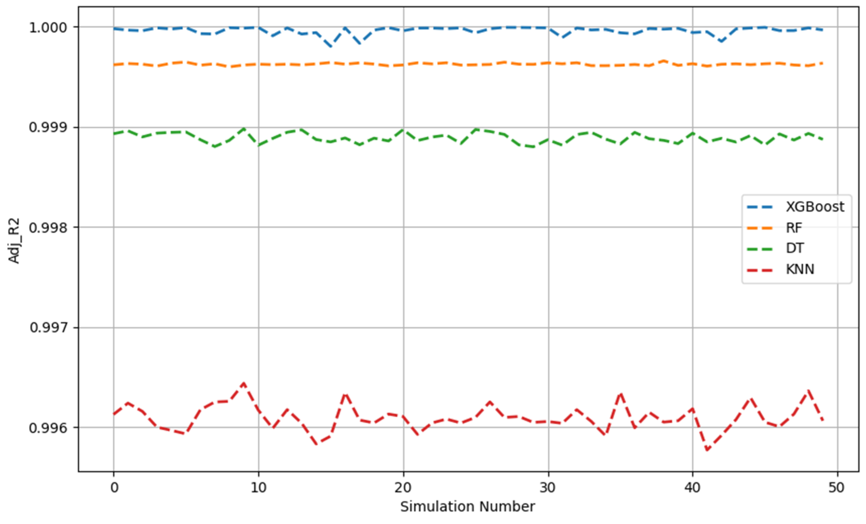
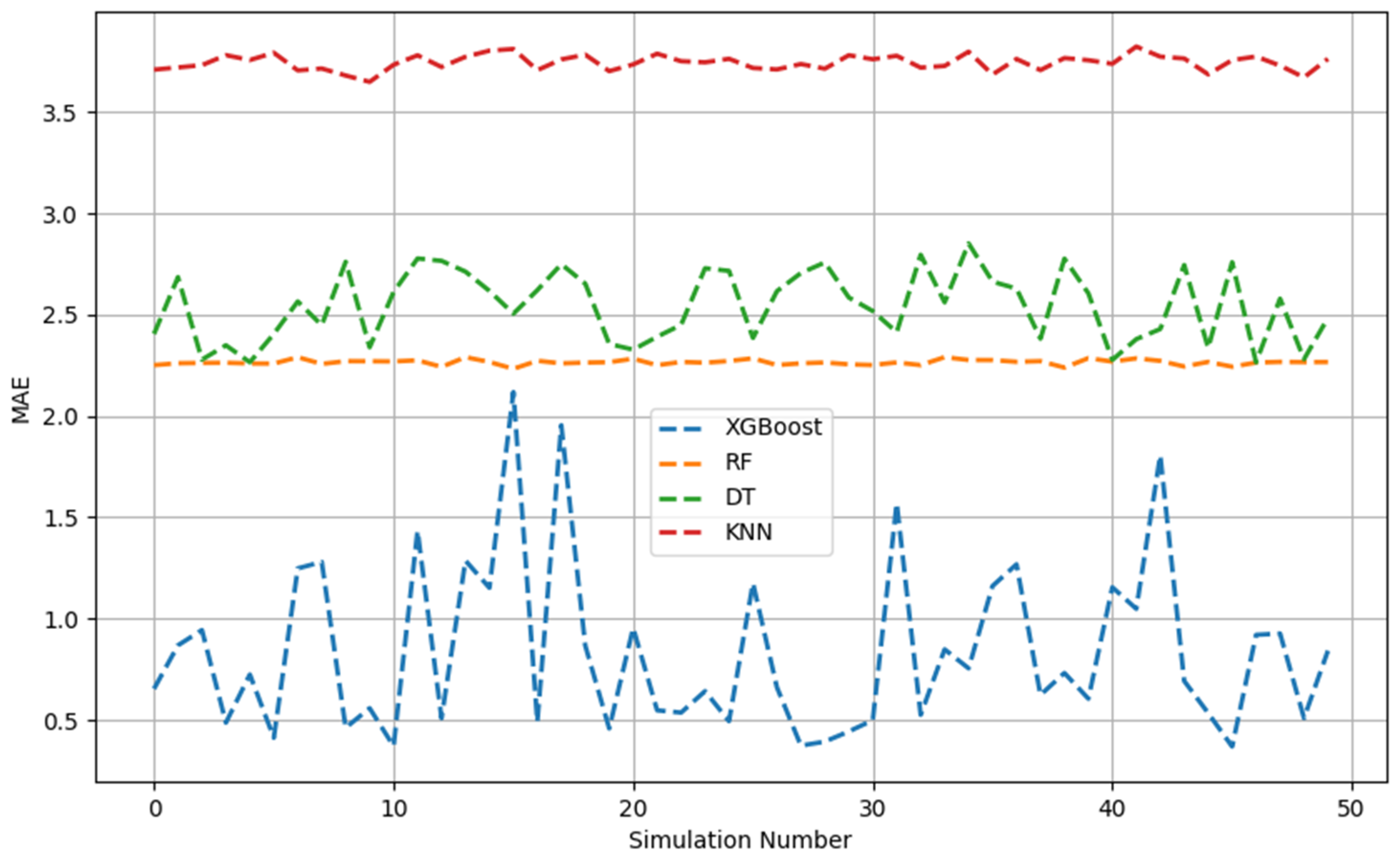
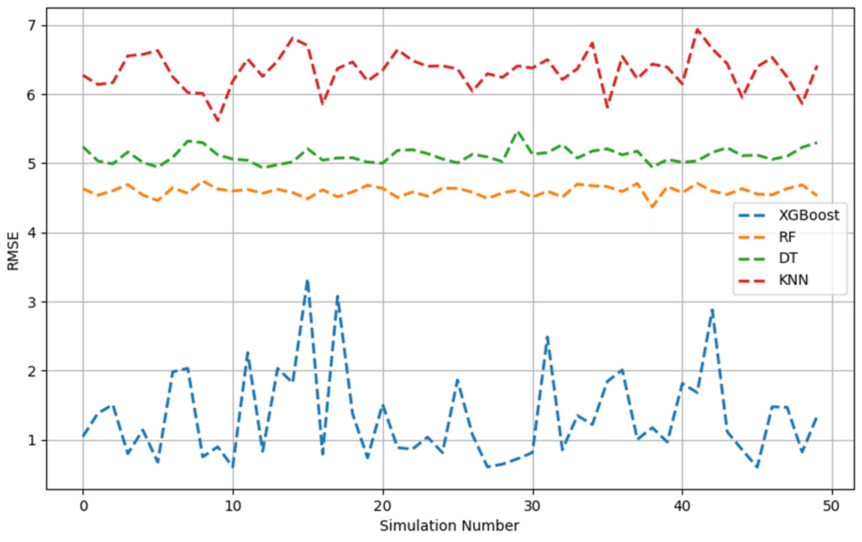
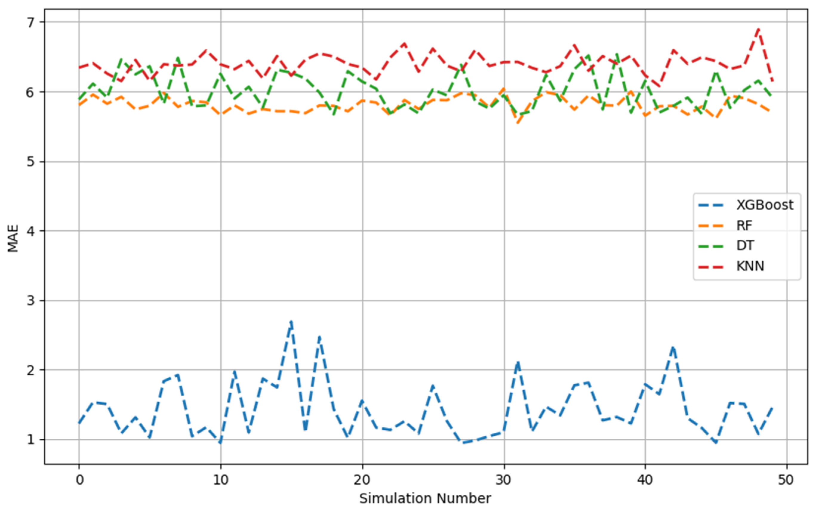
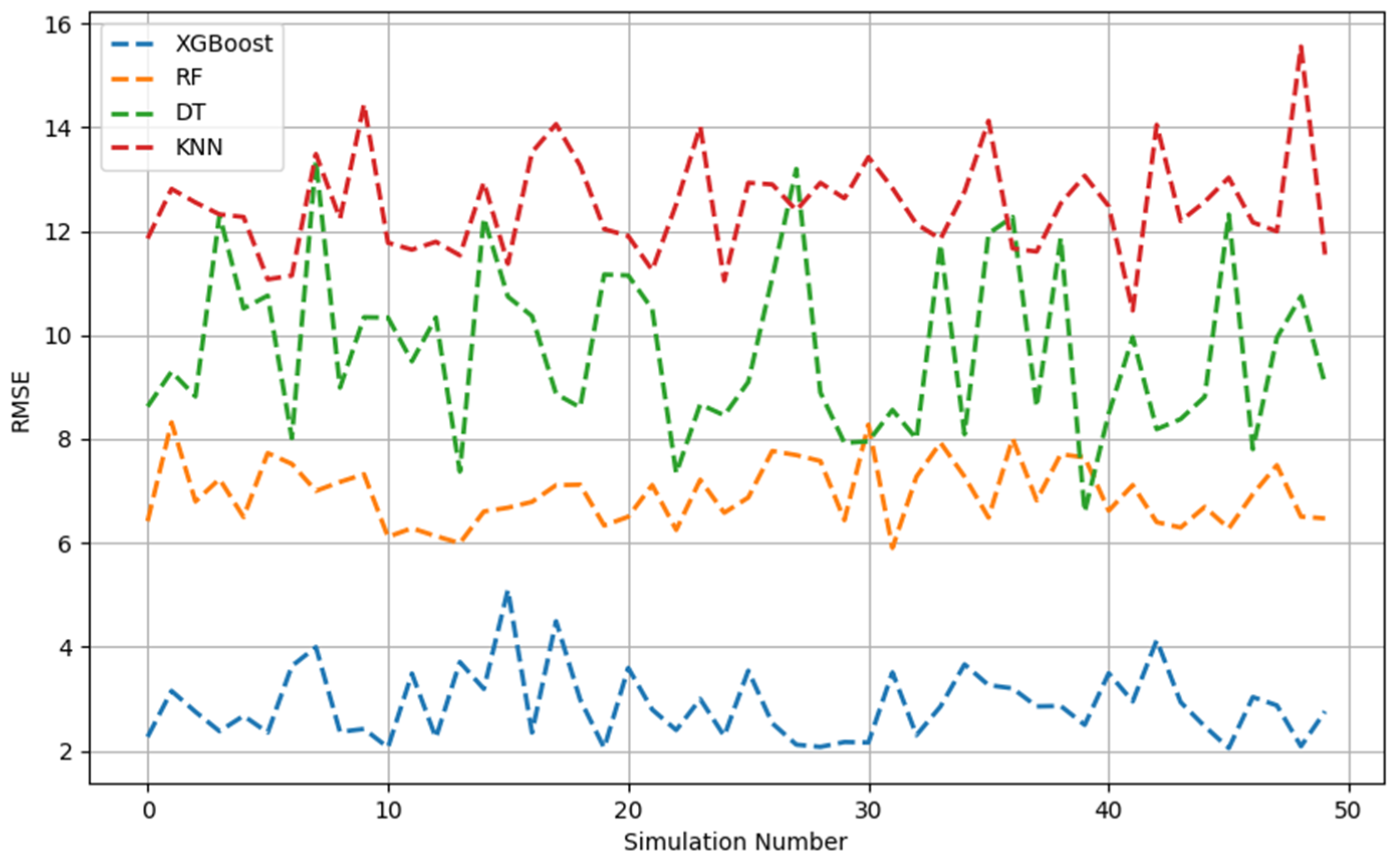
Figure 1, Figure 2, Figure 3, Figure 4, Figure 5 and Figure 6 show the 50 Monte Carlo simulation scores (adj. R2, MAE, and RMSE) for the training and testing stages, respectively, to assess the reliability of the XGBoost, RF, DT, and KNN models in estimating the methanol quantity needed. The scores in Figure 1, Figure 2 and Figure 3 corresponded only with the training dataset (80% of the dataset), and were used to illustrate the robustness of the models. The consistently high adj. R2 and low MAE and RMSE values indicated the overall good prediction ability of the proposed machine learning methods. The models were able to more accurately infer from the data after 50 runs and, overall, it was established that XGBoost had the highest predictive power. Based on the adj. R2 in the training stage, the models could be ordered according to performance as follows: KNN < DT < RF < XGBoost. The RF model had similar performance metrics to XGBoost. The KNN model showed less predictability and consistency than the other three ML models. Figure 1, Figure 2 and Figure 3 show the adj. R2, MAE, and RMSE values, respectively, of the training phase. The x-axis represents the sequence of scrambled datasets produced by the Monte Carlo method (1–50). For comparison, the vertical axis represents the values of the assessment criteria.
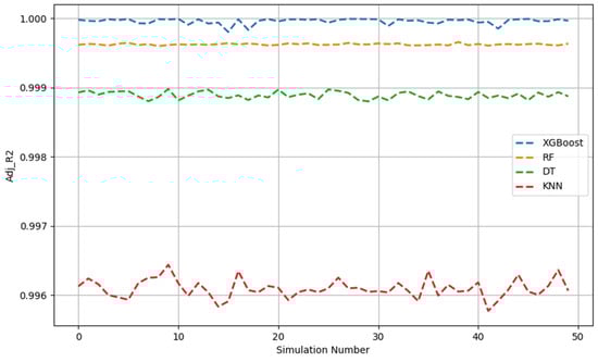
Figure 1.
Adj. R2 across 50 Monte Carlo simulations (training data).
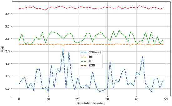
Figure 2.
MAE across 50 Monte Carlo simulations (training data).
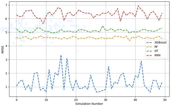
Figure 3.
RMSE across 50 Monte Carlo simulations (training data).
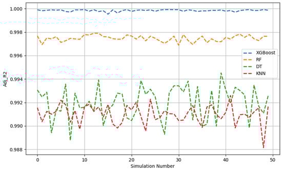
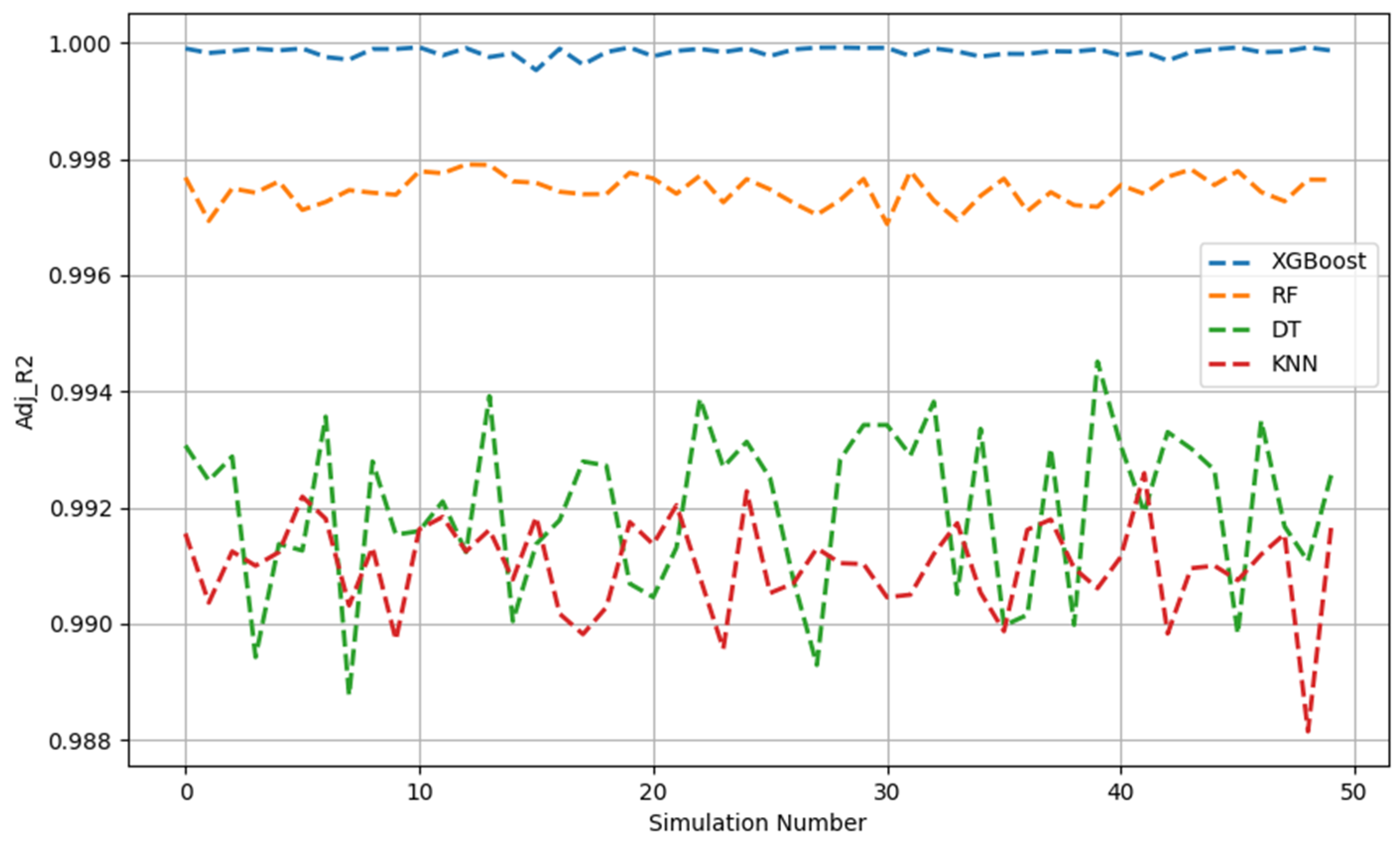
Figure 4.
Adj. R2 across 50 Monte Carlo simulations (testing data).
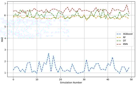
Figure 5.
MAE across 50 Monte Carlo simulations (testing data).
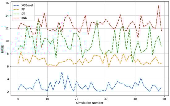
Figure 6.
RMSE across 50 Monte Carlo simulations (testing data).
The test stage, as illustrated in Figure 4, Figure 5 and Figure 6, revealed that, based on the decreasing order of the prediction performance of the models, the models ranked as follows: XGBoost, RF, DT, and KNN. This was similar to the preceding analyses. Overall, the XGBoost model demonstrated very strong predictive performance across 50 simulations, indexed by the relatively high adj. R2 values and low RMSE and MAE values. In contrast, the XGBoost model was much more consistent compared with the other three models given that, even after 50 iterations, the amplitude of the variation of all indicators was negligible.
The optimal performance features of the four ML models on the database are displayed in Table 2, which includes the testing and training datasets. Lower values for the MAE and RMSE implied a better predictive accuracy of the models. A higher adj. R2 value indicated a stronger fit of the model to explain the variance observed in the data. The results showed that, other than the KNN model, all ML models performed significantly better. The XGBoost and RF models had the lowest values for MAE and RMSE. This finding suggests that both methods could provide more accurate estimates of methanol volume with a small margin of error. Overall, this work highlights the better performance of the DT algorithm compared with the KNN model, as indicated by the high adj. R2 and low MAE values. This confirmed that the models could be used to provide reliable methanol quantity values for samples of gas pipelines.
Table 2.
Best performance metrics of four models for training and testing datasets.
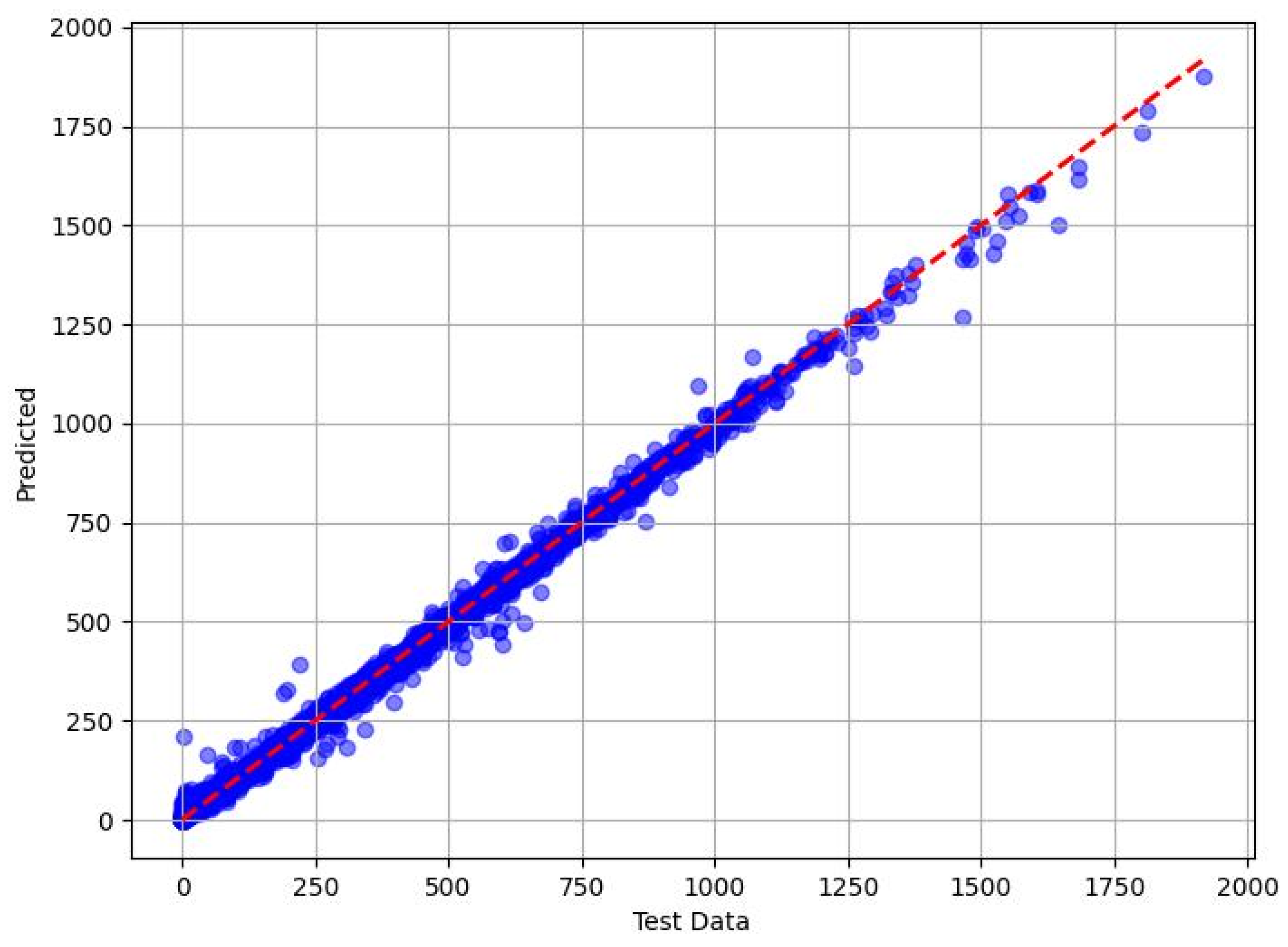
The scatter plots in Figure 7, Figure 8, Figure 9 and Figure 10 show the correlation between the measured methanol quantities and the predicted values from the XGBoost, RF, DT, and KNN models for gas pipeline samples. The XGBoost model exhibited exceptional predictive performance for determining the minimum methanol quantity required for hydrate inhibition. During the training phase, it achieved a mean absolute error (MAE) of 0.3693, indicating an average prediction error of just 0.3693 units compared with the actual methanol quantities in the training dataset. This low MAE underscored XGBoost’s ability to closely fit the training data. In the testing phase, the MAE slightly increased to 0.943, reflecting a modest rise in prediction errors when applied to unseen data, yet still demonstrating high accuracy. The RMSE further supported this with values of 0.6023 (training) and 2.066 (testing), indicating that larger errors, while present, remained minimal and manageable. The adj. R2 metric, which measured the proportion of variance in the target variable explained by the input features, was 0.999 for both the training and testing phases. This near-perfect score suggests that XGBoost captured 99.9% of the variability in methanol requirements, reflecting its robust fit with the training data and excellent generalization to the test set. These results highlight XGBoost’s superior reliability and precision in predicting methanol quantities across diverse pipeline conditions.
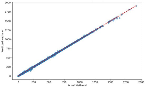
Figure 7.
Predicted vs. measured minimum methanol for hydrate inhibition by XGBoost (test dataset).
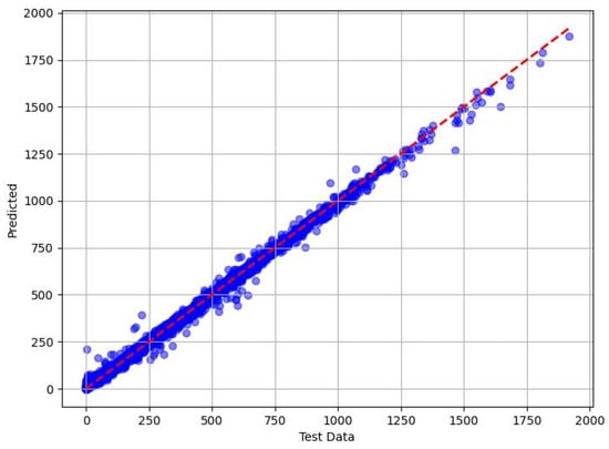
Figure 8.
Predicted vs. measured minimum methanol for hydrate inhibition by RF (test dataset).
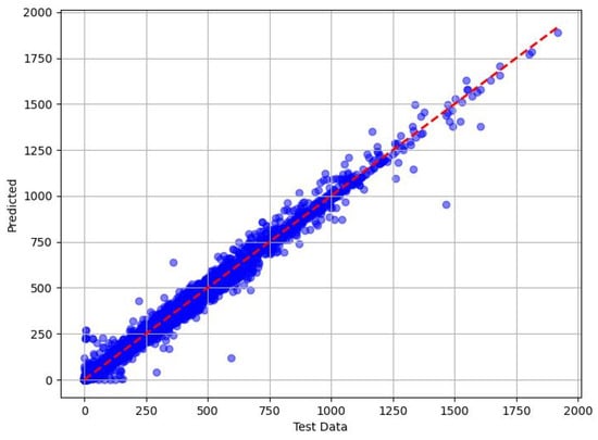
Figure 9.
Predicted vs. measured minimum methanol for hydrate inhibition by DT (test dataset).
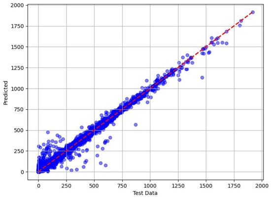
Figure 10.
Predicted vs. measured minimum methanol for hydrate inhibition by KNN (test dataset).
The random forest (RF) model also demonstrated a strong predictive capability, although it underperformed compared with XGBoost. During training, RF achieved an MAE of 2.238, meaning its predictions deviated from the actual methanol quantities by an average of 2.238 units, a respectable error margin that indicated good alignment with the training data. However, in the testing phase, the MAE rose to 5.680, suggesting a noticeable drop in accuracy when generalizing new data. This trend was mirrored in the RMSE values, which increased from 4.369 (training) to 6.13 (testing), indicating that RF was more susceptible to larger errors with unseen data compared with XGBoost. Despite this, RF maintained high adj. R2 values of 0.999 (training) and 0.997 (testing), demonstrating that it explained nearly all the variance in methanol quantities during training and retained strong explanatory power for the test set. Although RF performed well overall, its higher error metrics relative to XGBoost suggest that it was less consistent and precise for this application.
The decision tree (DT) model delivered solid but less impressive results compared with XGBoost and RF. In the training phase, it recorded an MAE of 2.339, reflecting an average error of 2.339 units and indicating reasonable accuracy in fitting the training data. During testing, the MAE increased to 5.695, revealing a decline in predictive accuracy for unseen data, consistent with DT’s tendency to overfit simpler tree structures. The RMSE values reinforced this pattern, rising from 5.12 (training) to 6.594 (testing), which pointed to a greater incidence of larger errors compared with the ensemble methods. The adj. R2 scores of 0.998 (training) and 0.994 (testing) remained high, indicating that DT explained most of the variance in methanol quantities and retained a decent generalization ability. However, its performance lagged behind XGBoost and RF, likely due to its lack of ensemble averaging, which limited its capacity to handle the dataset’s complexity as effectively.
The k-nearest neighbors (KNN) model showed the weakest performance among the four models evaluated. During training, it achieved an MAE of 3.648, corresponding with an average prediction error of 3.648 units, which was notably higher than the other models and suggested a poorer fit with the training data. In the testing phase, the MAE increased to 6.07, indicating a significant decline in accuracy when predicting methanol quantities for new pipeline scenarios. The RMSE values further highlighted KNN’s limitations, escalating from 5.619 (training) to 10.475 (testing), reflecting a substantial increase in both the frequency and magnitude of prediction errors for the test set. Despite this, KNN’s adj. R2 scores of 0.996 (training) and 0.992 (testing) indicated that it still explained a high proportion of the variance in methanol requirements, although its explanatory power was the lowest among the models. KNN’s inferior performance could be attributed to its reliance on local similarity, which struggled with the nonlinear relationships and high-dimensional feature space of this dataset, making it less suitable for precise methanol dosing predictions.
3.2. Feature Importance Analysis
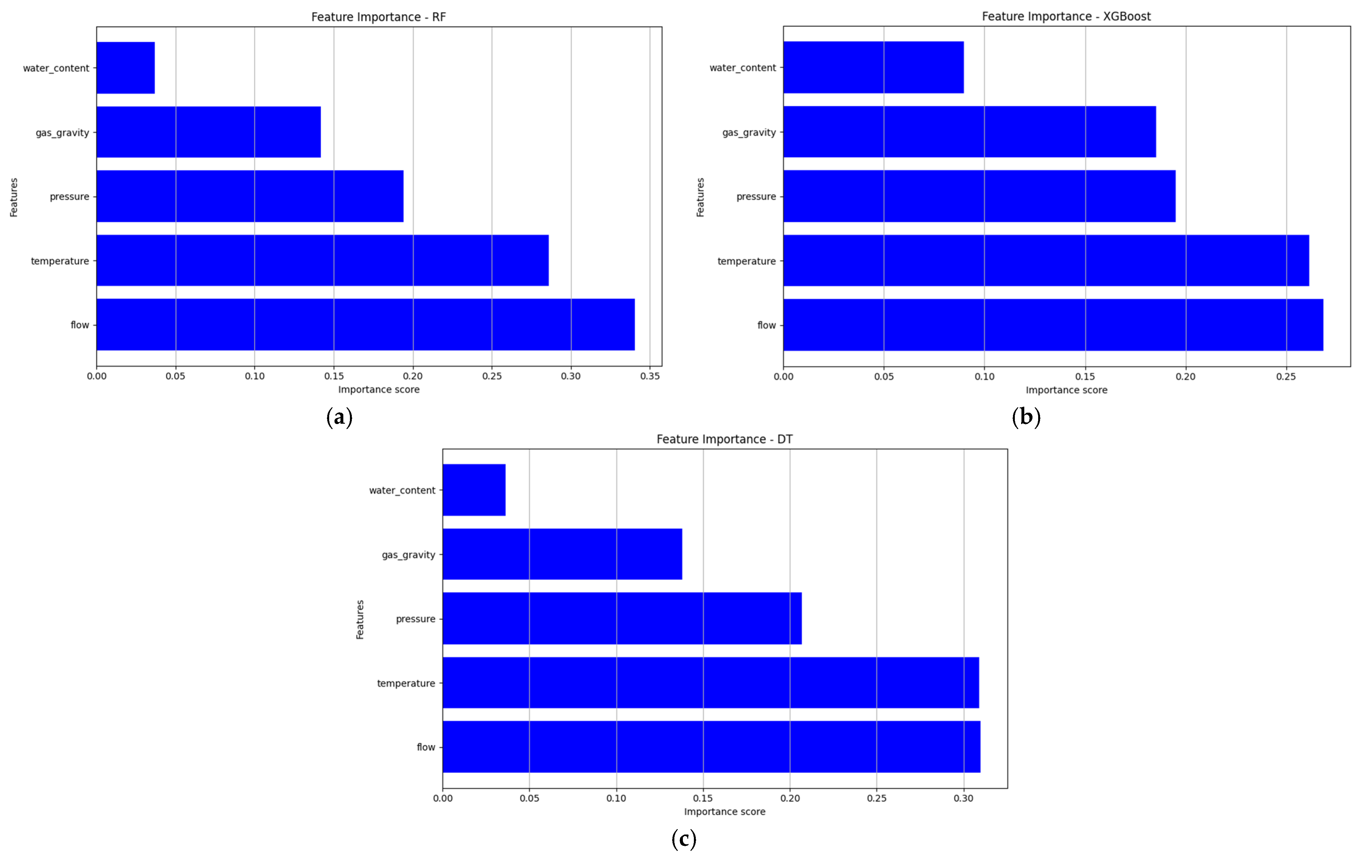
The feature importance analysis conducted for the XGBoost, RF, and DT models using the full dataset elucidated the relative contributions of the five input features of flow rate, temperature, pressure, gas specific gravity, and water content to predict the minimum methanol quantity required for hydrate inhibition (Figure 11). This analysis, derived from the models’ intrinsic Gini importance scores via scikit-learn and XGBoost in PyCharm [33], provided critical insights into the key drivers of methanol dosing, aiding the operational optimization of gas pipelines.
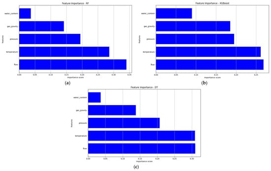
Figure 11.
Feature importance scores: (a) RF; (b) XGBoost; (c) DT.
The most influential feature across all three models was found to be flow rate, with importance scores of approximately 0.34 (RF), 0.27 (XGBoost), and 0.31 (DT), highlighting the dominant role of flow rate in driving methanol distribution and hydrate inhibition requirements [26]. The next most important feature was temperature, with scores of 0.28 (RF), 0.27 (XGBoost), and 0.31 (DT) due to its influence on the phase equilibrium and overall hydrate stability according to different pipeline parameters [2]. Pressure fell as a moderate importance feature, with a static score of 0.20 across RF, XGBoost, and DT, which was reasonable, based on the influence it has over the gas–water phase [6]. Gas specific gravity was given importance scores of 0.14 (RF), 0.18 (XGBoost), and 0.14 (DT), emphasizing a secondary role in the methanol needs of lean gas systems [38]. Water content showed the least impact, with scores of 0.05 (RF), 0.08 (XGBoost), and 0.04 (DT), suggesting its minimal contribution to methanol prediction in this context [27].
These results indicated that flow rate and temperature were the primary determinants of methanol dosing, aligning with the dynamic flow and thermal conditions critical for hydrate inhibition [4]. The consistency in feature rankings across models validated their reliability, although minor variations (e.g., slightly higher water-content importance for XGBoost and DT) suggested model-specific sensitivities, potentially due to differences in tree structures [29]. This analysis could enable engineers to prioritize optimizing flow rate and temperature control to enhance methanol efficiency, improving pipeline safety and cost-effectiveness in hydrate management.
3.3. Correlation Matrix of Input Features and Methanol Injection Rate
To explore the relationships between the five input features (flow rate, temperature, pressure, gas specific gravity, and water content) and the minimum methanol injection rate required, a correlation matrix analysis was conducted. Visualized in Figure 12, this analysis used Pearson correlation coefficients (r) from −1 to 1 to quantify linear dependencies, shedding light on the feature influences on methanol dosing for hydrate inhibition. These findings complemented the machine learning models’ predictions and feature importance analysis, offering a linear perspective to guide operational decisions.
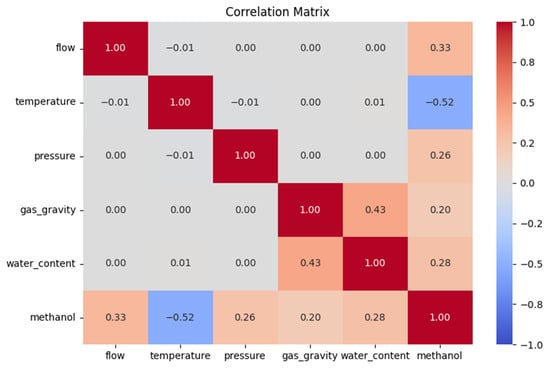
Figure 12.
Correlation matrix of input features and methanol injection rate.
The matrix revealed clear patterns in methanol correlations. Flow rate showed the strongest positive correlation (r = 0.33), indicating that higher flows increase methanol needs due to elevated hydrate risks and distribution demands [4]. Temperature exhibited a moderate negative correlation (r = −0.52), suggesting that lower temperatures raise methanol requirements by stabilizing hydrates [3]. Pressure (r = 0.26), gas specific gravity (r = 0.20), and water content (r = 0.28) showed weaker positive correlations, reflecting milder effects. Water content’s modest r-value, despite its role in hydrate formation [26], likely reflected its narrow dataset range, limiting the linear impact.
Inter-feature correlations were near zero (e.g., flow rate vs. temperature; r = −0.01), confirming their independence and suitability as distinct predictors in ML models and minimizing multicollinearity [17]. These results aligned with Section 3.2, where flow rate and temperature dominated across the XGBoost, RF, and DT models, although water content’s weaker linear role highlighted ML’s nonlinear strength.
Practically, this can inform methanol dosing. Flow rate adjustments significantly affect inhibitor needs, while temperature management reduces use in colder sections. Pressure, specific gravity, and water content play secondary roles. Integrating these insights with ML predictions optimizes hydrate prevention, balancing costs and environmental efficiency in gas pipelines.
4. Conclusions
This study assessed the performance of four machine learning models (XGBoost, RF, DT, and KNN) in predicting the minimum methanol quantity needed for gas hydrate inhibition in pipelines, utilizing a synthetic dataset of 74,000 samples generated from Aspen HYSYS simulations. The dataset was divided into an 80% training set and a 20% testing set, with model robustness enhanced using Monte Carlo simulations and tenfold cross-validation. Evaluation metrics revealed that XGBoost consistently outperformed the other models, demonstrating the highest accuracy and reliability in both the training and testing phases. RF ranked second, delivering strong predictive capability, although it was less consistent than XGBoost. This was followed by DT, with moderate performance, and KNN exhibited the weakest results. This established a clear performance hierarchy of XGBoost surpassing RF, DT, and KNN, with XGBoost excelling in fitting the training data and generalizing unseen pipeline scenarios.
A feature importance analysis across the tree-based models (XGBoost, RF, and DT) identified flow rate and temperature as the most influential factors in determining methanol requirements, reflecting their critical roles in methanol distribution and hydrate stability, respectively. Pressure, gas specific gravity and water content were not as influential, with water content being the least important, likely because there was not as much variety in the dataset. These results were consistent with that of the correlation analysis, which indicated a strong positive relationship between flow rate and methanol needs, a strong negative relationship with temperature, and a weaker positive relationship with pressure, gas specific gravity, and water content. These analyses characterized flow rate and temperature as the two primary parameters informing the optimal approach to methanol injection in gas transportation pipelines.
XGBoost’s excellent performance positioned it as a potentially useful tool to tackle oil and gas problems, surpassing what a traditional empirical approach could have achieved and being less resource-demanding than a simulation process such as Aspen HYSYS. It could aid pipeline safety while lowering the operational costs and environmental impacts associated with over-dosing by offering accurate, adaptable forecasts of methanol requirements. However, as the study relied on synthetic data, its real-world applicability is limited, and validation using operational pipeline data is needed to confirm these findings. This study addressed a significant need in hydrate inhibition studies, suggesting machine learning’s ability to act as an efficient, data-first approach to inhibitor optimization. Therefore, the combination of ML and high-fidelity simulation data lays the groundwork for a new and versatile platform to improve methanol management, with relevance beyond the simple mitigation of hydrate formation to larger process engineering problems. As the industry shifts toward data-centric approaches, XGBoost represents a key enabler in driving the evolution of more efficient and sustainable gas transportation systems, pending such validations.
5. Limitations and Future Work
The study, like many machine learning studies, was not without its limitations. Based on synthetic data from 20 gas compositions simulated by Aspen HYSYS, the investigation limited the findings and predictions to the conditions of the simulations and not the real-world environment of a pipeline. This reliance on synthetic data restricted the models’ proven applicability to operational settings because real pipeline conditions could introduce complexities (e.g., unmodeled impurities) not captured here. The other limitation was that the dataset had limited features; although the proposed models demonstrated good performance in this regard, they may not hold as well for wider or narrower datasets and, therefore, should be used with caution outside this boundary. In addition, the models were highly reliant on the input parameters of flow rate, temperature, pressure, gas specific gravity, and water content, which were optimized for the ranges of this study. However, applying these models outside these ranges (such as extreme temperatures or pressures) may yield erroneous results because they have not been verified for these conditions.
Future machine learning studies for predicting methanol demand for hydrate control need to include more diverse and detailed datasets, including data from real gas pipelines, to improve the generalizability and strength of the models. Validation using operational pipeline data is essential to confirm the accuracy and practical utility of XGBoost and other models, addressing the current gap between synthetic and real-world performance. Increasing both the diversity of models and the dataset could lead to more generalizable machine learning models. This would enhance their ability to be used more widely across a variety of pipeline conditions and gas compositions. Integrating new machine learning techniques like deep learning may also improve the error levels that KNN was unable to resolve, allowing the modeling of a much wider range of processes involved in hydrate inhibition processes, such as how different input parameters (for example, inhibitor type or pipeline geometry) affect hydrate inhibition behavior.
Author Contributions
Conceptualization, W.L. and M.H.M.; methodology, M.H.M.; software, M.H.M.; validation, W.L.; formal analysis, M.H.M.; investigation, W.L., M.H.M., and G.H.J.; resources, G.H.J.; data curation, M.H.M.; writing—original draft preparation, M.H.M.; writing—review and editing, M.H.M.; visualization, M.H.M.; supervision, W.L. All authors have read and agreed to the published version of the manuscript.
Funding
This research received no external funding.
Institutional Review Board Statement
Not applicable.
Informed Consent Statement
Not applicable.
Data Availability Statement
The raw data supporting the conclusions of this article will be made available by the authors upon request.
Conflicts of Interest
The authors declare no conflicts of interest.
Abbreviations
The following abbreviations are used in this manuscript:
| XGBoost | Extreme Gradient Boosting |
| RF | Random Forest |
| DT | Decision Tree |
| KNN | K-Nearest Neighbors |
| Adj. R2 | Adjusted R-Squared |
| MAE | Mean Absolute Error |
| RMSE | Root Mean Square Error |
| ML | Machine Learning |
| HFT | Hydrate Formation Temperature |
| HFP | Hydrate Formation Pressure |
| ANN | Artificial Neural Network |
| SVM | Support Vector Machine |
References
- Holechek, J.; Geli, H.; Sawalhah, M.; Valdez, R. A global assessment: Can renewable energy replace fossil fuels by 2050? Sustainability 2022, 14, 4792. [Google Scholar] [CrossRef]
- Sloan, E.D., Jr.; Koh, C.A. Clathrate Hydrates of Natural Gases; CRC Press: Boca Raton, FL, USA, 2007. [Google Scholar]
- Makogon, Y.F. Hydrates of Hydrocarbons; PennWell Books: Tulsa, OK, USA, 1997. [Google Scholar]
- Hammerschmidt, E. Formation of gas hydrates in natural gas transmission lines. Ind. Eng. Chem. 1934, 26, 851–855. [Google Scholar] [CrossRef]
- Aman, Z.M. Hydrate risk management in gas transmission lines. Energy Fuels 2021, 35, 14265–14282. [Google Scholar] [CrossRef]
- Carroll, J. Natural Gas Hydrates: A Guide for Engineers; Gulf Professional Publishing: Waltham, MA, USA, 2020. [Google Scholar]
- Anderson, B.J.; Tester, J.W.; Borghi, G.P.; Trout, B.L. Properties of inhibitors of methane hydrate formation via molecular dynamics simulations. J. Am. Chem. Soc. 2005, 127, 17852–17862. [Google Scholar] [CrossRef] [PubMed]
- Ismail, I.; Gaganis, V. Prediction of Hydrate Dissociation Conditions in Natural/Acid/Flue Gas Streams in the Presence and Absence of Inhibitors. Mater. Proc. 2024, 15, 73. [Google Scholar] [CrossRef]
- Giavarini, C.; Hester, K. Gas Hydrates: Immense Energy Potential and Environmental Challenges; Springer Science & Business Media: Berlin, Germany, 2011. [Google Scholar] [CrossRef]
- Davarnejad, R.; Azizi, J.; Azizi, J. Prediction of gas hydrate formation using HYSYS software. Int. J. Eng.-Trans. C Asp. 2014, 27, 1325–1330. [Google Scholar] [CrossRef]
- Carroll, J. Inhibiting hydrate formation with chemicals. In Natural Gas Hydrates; Gulf Professional Publishing: Waltham, MA, USA, 2020; pp. 163–208. [Google Scholar]
- Owolabi, J.O.; Kila, O.O.; Giwa, A. Modelling and Simulation of a Natural Gas Liquid Fractionation System Using Aspen HYSYS. Int. J. Eng. Res. Afr. 2020, 49, 1–14. [Google Scholar] [CrossRef]
- Abbasi, A.; Hashim, F.M. A review on fundamental principles of a natural gas hydrate formation prediction. Pet. Sci. Technol. 2022, 40, 2382–2404. [Google Scholar] [CrossRef]
- Proshutinskiy, M.; Raupov, I.; Brovin, N. Algorithm for optimization of methanol consumption in the «gas inhibitor pipeline-well-gathering system». In Proceedings of the IOP Conference Series: Earth and Environmental Science; IOP: Bristol, UK, 2022. [Google Scholar]
- Lu, Y.; Shen, M.; Wang, H.; Wang, X.; van Rechem, C.; Fu, T.; Wei, W. Machine learning for synthetic data generation: A review. arXiv 2023, arXiv:2302.04062. [Google Scholar]
- Alpaydin, E. Introduction to Machine Learning; MIT Press: Cambridge, MA, USA, 2020. [Google Scholar]
- Hastie, T.; Tibshirani, R.; Friedman, J.H.; Friedman, J.H. The Elements of Statistical Learning: Data Mining, Inference, and Prediction; Springer: New York, NY, USA, 2009; Volume 2. [Google Scholar]
- Jordan, M.I.; Mitchell, T.M. Machine learning: Trends, perspectives, and prospects. Science 2015, 349, 255–260. [Google Scholar] [CrossRef]
- El-hoshoudy, A.; Ahmed, A.; Gomaa, S.; Abdelhady, A. An artificial neural network model for predicting the hydrate formation temperature. Arab. J. Sci. Eng. 2022, 47, 11599–11608. [Google Scholar] [CrossRef]
- Ibrahim, A.A.; Lemma, T.A.; Kean, M.L.; Zewge, M.G. Prediction of gas hydrate formation using radial basis function network and support vector machines. Appl. Mech. Mater. 2016, 819, 569–574. [Google Scholar] [CrossRef]
- Cao, J.; Zhu, S.; Li, C.; Han, B. Integrating support vector regression with genetic algorithm for hydrate formation condition prediction. Processes 2020, 8, 519. [Google Scholar] [CrossRef]
- Nasir, Q.; Suleman, H.; Abdul Majeed, W.S. Application of Machine Learning on Hydrate formation prediction of pure components with water and inhibitors solution. Can. J. Chem. Eng. 2024, 102, 3953–3981. [Google Scholar] [CrossRef]
- Nasir, Q.; Abdul Majeed, W.S.; Suleman, H. Predicting Gas Hydrate Equilibria in Multicomponent Systems with a Machine Learning Approach. Chem. Eng. Technol. 2023, 46, 1854–1867. [Google Scholar] [CrossRef]
- Hajjeyah, A.; Al-Saleh, A.; Al-Qahtan, S.; Al-Shuaib, M.; Al-Muhanna, D.; Al-Jarki, D.; Al-Salali, Y.Z.; Osaretin, G.I.; Mahmoud, M.M.; Sabat, S. Enhancing Production Efficiency: AI-Powered Hydrate Detection and Prevention in North Kuwait Jurassic Gas Field. In Proceedings of the Abu Dhabi International Petroleum Exhibition and Conference, Abu Dhabi, United Arab Emirates, 4–7 November 2024. [Google Scholar]
- Salam, K.; Arinkoola, A.; Araromi, D.; Ayansola, Y. Prediction of Hydrate formation conditions in Gas pipelines. Int. J. Eng. Sci. 2013, 2, 327–331. [Google Scholar]
- Sloan, E.D. Natural Gas Hydrates in Flow Assurance; Gulf Professional Publishing: Waltham, WA, USA, 2010. [Google Scholar]
- Mokhatab, S.; Poe, W.A.; Mak, J.Y. Handbook of Natural Gas Transmission and Processing: Principles and Practices; Gulf Professional Publishing: Waltham, WA, USA, 2018. [Google Scholar]
- Raschka, S.; Liu, Y.H.; Mirjalili, V. Machine Learning with PyTorch and Scikit-Learn: Develop Machine Learning and Deep Learning Models with Python; Packt Publishing Ltd.: Birmingham, UK, 2022. [Google Scholar]
- Biau, G.; Scornet, E. A random forest guided tour. Test 2016, 25, 197–227. [Google Scholar] [CrossRef]
- De Clercq, D.; Smith, K.; Chou, B.; Gonzalez, A.; Kothapalle, R.; Li, C.; Dong, X.; Liu, S.; Wen, Z. Identification of urban drinking water supply patterns across 627 cities in China based on supervised and unsupervised statistical learning. J. Environ. Manag. 2018, 223, 658–667. [Google Scholar] [CrossRef]
- Feng, M.; Wang, X.; Zhao, Z.; Jiang, C.; Xiong, J.; Zhang, N. Enhanced Heart Attack Prediction Using eXtreme Gradient Boosting. J. Theory Pract. Eng. Sci. 2024, 4, 9–16. [Google Scholar] [CrossRef]
- Probst, P.; Wright, M.N.; Boulesteix, A.L. Hyperparameters and tuning strategies for random forest. Wiley Interdiscip. Rev. Data Min. Knowl. Discov. 2019, 9, e1301. [Google Scholar] [CrossRef]
- Ali, A.; Hamraz, M.; Kumam, P.; Khan, D.M.; Khalil, U.; Sulaiman, M.; Khan, Z. A k-nearest neighbours based ensemble via optimal model selection for regression. IEEE Access 2020, 8, 132095–132105. [Google Scholar] [CrossRef]
- Bergstra, J.; Komer, B.; Eliasmith, C.; Yamins, D.; Cox, D.D. Hyperopt: A python library for model selection and hyperparameter optimization. Comput. Sci. Discov. 2015, 8, 014008. [Google Scholar] [CrossRef]
- Dao, D.V.; Trinh, S.H.; Ly, H.-B.; Pham, B.T. Prediction of compressive strength of geopolymer concrete using entirely steel slag aggregates: Novel hybrid artificial intelligence approaches. Appl. Sci. 2019, 9, 1113. [Google Scholar] [CrossRef]
- Fatah, T.A.; Mastoi, A.K.; Bhatti, N.-u.-K.; Ali, M. Optimizing Stabilization of Contaminated Mining Sludge: A Machine Learning Approach to Predict Strength and Heavy Metal Leaching. Arab. J. Sci. Eng. 2024, 1–21. [Google Scholar] [CrossRef]
- Shen, K.-Q.; Ong, C.-J.; Li, X.-P.; Wilder-Smith, E.P. Feature selection via sensitivity analysis of SVM probabilistic outputs. Mach. Learn. 2008, 70, 1–20. [Google Scholar] [CrossRef]
- Tohidi, B.; Burgass, R.; Danesh, A.; Todd, A. Hydrate inhibition effect of produced water: Part 1—Ethane and propane simple gas hydrates. In Proceedings of the SPE Offshore Europe Conference and Exhibition, Aberdeen, UK, 7–10 September 1993. [Google Scholar]


Disclaimer/Publisher’s Note: The statements, opinions and data contained in all publications are solely those of the individual author(s) and contributor(s) and not of MDPI and/or the editor(s). MDPI and/or the editor(s) disclaim responsibility for any injury to people or property resulting from any ideas, methods, instructions or products referred to in the content. |
© 2025 by the authors. Licensee MDPI, Basel, Switzerland. This article is an open access article distributed under the terms and conditions of the Creative Commons Attribution (CC BY) license (https://creativecommons.org/licenses/by/4.0/).