Dynamic Energy Consumption Modeling for HVAC Systems in Electric Vehicles

Abstract

Motivated by the strong transition to electric mobility we are witnessing currently, in this paper, we present a novel methodology to predict the dynamic behavior of heat, ventilation and air conditioning (HVAC) systems for electric vehicles. The approach is based on a lumped parameter energy balance between the vehicle cabin, the external loads (such as solar radiation, ventilation and metabolic load) and the HVAC system. Detailed models are used to obtain the time evolution of the heat transfer coefficients of each subsystem in the HVAC (i.e., evaporator and condenser) on the basis of correlations available in the literature. The model is validated on a real HVAC system, built ad hoc for a retrofitted electric vehicle, by comparing the results obtained from the model with experimental measurements performed in a climatic chamber. Then, some scenarios that represent interesting cases in electric automotive applications, such as vehicle cabin precooling during battery charging and a regulated driving cycle which simulates urban mobility, are considered. The energy consumption of the HVAC system is evaluated from the model in these scenarios and compared. The methodology herein presented is general and easily extendable to other systems, proving to be a powerful method to compare the energy consumption of HVAC systems under unsteady conditions with a more standard approach based on steady considerations. By this approach, it is shown that significant improvement can be obtained with a nonsteady approach.

1. Introduction

The development of electric mobility we are witnessing in the present years requires a parallel improvement in sustainable technologies integrated into vehicles, with the aim of energy savings. The heating, ventilation and air conditioning system (HVAC) is one of the most energy-consuming appliances in a vehicle. The design and the energy consumption assessment of HVAC systems for automotive systems are usually based on steady-state approaches, where the subsystems (such as the evaporator, the condenser and the compressor) are described by proper correlations. However, HVAC works always under unsteady conditions, as in a vehicle, the thermal loads are continuously changing during driving. Therefore, it is crucial to obtain a model capable of describing the behavior of an HVAC system under unsteady conditions to perform a full assessment of the energy exchanged between the subsystems (such as the evaporator, the condenser and the compressor) during the working cycle and the interaction between the vehicle cabin and the external environment. This model can give different results with respect to the usual steady-state modeling approaches, which assume that the variables of interest do not change over time. Some works are available in the literature on dynamical modeling of HVAC systems. Catano et al. [1] present a lumped parameter dynamic model of a vapor compression cycle used for electronic cooling. In this model, the dynamics of heat exchangers is coupled with static empirical models of the compressor and expansion valve. The model is validated by comparison with experiments under different operating conditions. Performance optimization is achieved by obtaining the minimum compressor power consumption together with the maximum critical heat flux. Nunes et al. [2] introduce a simplified dimensionless model to describe the transient behavior of a vapor compression refrigeration system. The purpose of the study is to optimize the heat transfer area of the heat exchangers, minimizing the system pull-down time. Heimel et al. [3] propose a 1D transient model for refrigeration systems where the subcomponents are independently validated. The method is applied to a domestic freezer and tested under varying ambient temperatures and thermostat settings. Yin et al. [4] present an optimization strategy for the vapor compression refrigeration cycle, which by analyzing the characteristics and interactions of each component within the cycle minimizes the total operating cost of the energy-consuming devices subject to the constraints of mechanical limitations, component interactions, environment conditions and cooling load demands. Recent works deal with model predictive control strategies to optimize the operation of the thermal management system by intelligently managing the energy allocation between different components [5]. Liang et al. [6] review the literature on integrated thermal management systems for electric vehicles. They first introduce the research status of each subsystem then focus on the analysis of the advances to obtain the performance evaluation of the integrated systems shown. The discussed solutions, however, are characterized by experimental studies, showing the need of validated dynamic simulations to support the prototyping phase. Ibrahim and Jiang [7] provide a comprehensive discussion on electric vehicle energy management systems, focusing on equivalent circuit models and discussing associated simulation resources and software packages. They also present an illustrative case study on the thermal modeling and simulation of lithium ion batteries using the equivalent circuit model. The dynamic simulation of HVAC systems for automotive applications has only recently appeared in the literature. Zhao et al. [8] present a review related to the modeling of the cabin thermal environment. The results indicate that the primary modeling methods used in this field are Computational Fluid Dynamics (CFD) and lumped parameter methods, accounting for the majority of the surveyed literature. Additionally, data-driven approaches utilizing machine learning techniques have gained increasing attention due to the rapid development of machine learning. Among the studies surveyed, solar radiation, cabin occupants and vehicle driving conditions are the primary factors considered when modeling vehicle thermodynamics. However, the influence of humidity is largely overlooked despite its potential correlation with the thermal environment and passenger comfort. They identify two major research gaps: the need for a well-balanced trade-off between model complexity and accuracy, which can be used for optimal control of the cabin thermal environment in real time, and the absence of standardized boundary conditions to compare and validate various models. They identify three promising directions for future research: the development of control-oriented simulation techniques, the establishment of a standardized model repository that captures typical internal and external thermal characteristics of automotive cabins and the utilization of machine learning algorithms to develop surrogate models of the cabin thermal environment. The review reveals a notable gap in the dynamic analysis of HVAC system elements. He et al. [9] analyze the distribution of heat sources in the vehicle, the requirements of the heat load, the modeling approaches for the main thermal management system, the control methods and the developments of refrigerants from the perspective of the entire vehicle. Finally, they conclude that there is still much work to do and that the electric vehicle thermal management system will develop toward integration and efficiency in the future. Karimshoushtari et al. [10] introduce three advanced model-based control strategies for the cabin active heating thermal system of an EV, namely, linear and nonlinear. For this purpose, a physics-based model of the aforementioned thermal system is derived and validated using data generated from a high-fidelity thermal plant model created in GT-suite software. The parameters of the physics-based model are identified using some optimization algorithms. They show that the nonlinear dynamics of the thermal system has been accurately captured. A comprehensive test study is performed, and the performance of the proposed approaches is evaluated using various indicators such as reference tracking, energy consumption, robustness, computation time and implementation complexity. The results of the test study demonstrate the high performance and efficiency of the proposed control strategies, which offer significant advancements in the control of the thermal system of electrified vehicles. Narimani et al. [11] propose a unified thermal management framework, developed for the entire EV, which addresses both the heating and cooling requirements for the battery pack and the HVAC system of an electric vehicle. They present a detailed 1D simulation model in which different parts of the vehicle, including the powertrain components, battery pack, cabin, compressor, battery chiller, expansion valves, pumps, radiator fan, etc., are accurately modeled and integrated into the EV general model in the GT-Suite environment. Considering different heating/cooling scenarios in various environmental conditions (including air temperature, solar flux, metabolic rate, vehicle speed, etc.), effective control systems are designed for each subsystem, particularly the compressor, heaters and pumps, using the gain-scheduling PI control method in the MATLAB/Simulink R2023B environment coupled with the GT-Suite model. They show that the system can maintain the battery temperature within a range while reducing the cabin temperature. They show preliminary tests conducted on an actual vehicle to evaluate its performance under real-world driving conditions. The results obtained indicate that the suggested thermal management system is capable of tuning the battery temperature and cabin temperature in various conditions, complying with the protective rules required in real EVs. Finally, some works deal with the coupling between the dynamic analysis and the external environment. Lan et al. [12] analyze differences in spatial structure and environmental characteristics of urban roads to design environmental load spectrum tests for various road types, including open roads, boulevards and underground parking lots. The tests are conducted in a southern Chinese city to acquire characteristic parameters such as solar radiation, temperature and humidity for different urban microclimates in road spaces. Then, the effects on the thermal response of the cabin and the passengers’ cooling requirements are analyzed. Finally, cooling schemes are developed to match the specific urban microclimates of the road space, with the goal of thermal comfort and low energy consumption. The aim of this work is to model the transient behavior of a vapor compression refrigerating system for automotive use through a Matlab/Simulink code. The code is applied to a refrigeration system built for automobiles, working with R134a, and inserted into a simplified model of an electric car. The proposed innovative control strategy offers several advantages. It includes a comprehensive control-oriented model developed for simulating the HVAC system, capable of accurately capturing system dynamic performance using generalized correlations for the evaporator and condenser, which allows for the incorporation of additional control variables. The accuracy of this model is validated through experiments performed on a real device built for an electric vehicle. Furthermore, when applied within the developed model, the proposed control strategy demonstrates significant improvements in energy savings for the thermal management system compared to the PI control reference under the same temperature control standards. The model is applied to constant-velocity scenarios and the regulated ECE 15 driving cycle [13]. In this case, it is shown that the HVAC system considered increases the total energy consumption of the electric vehicle by about 40% of the total energy required to drive. The contribution of the HVAC system has been shown to be very important in the overall energy consumption of an electric vehicle. For this reason, a computational model that allows one to evaluate the electrical consumption due to the HVAC system is very important to improve the efficiency of electric mobility.

2. Materials and Methods

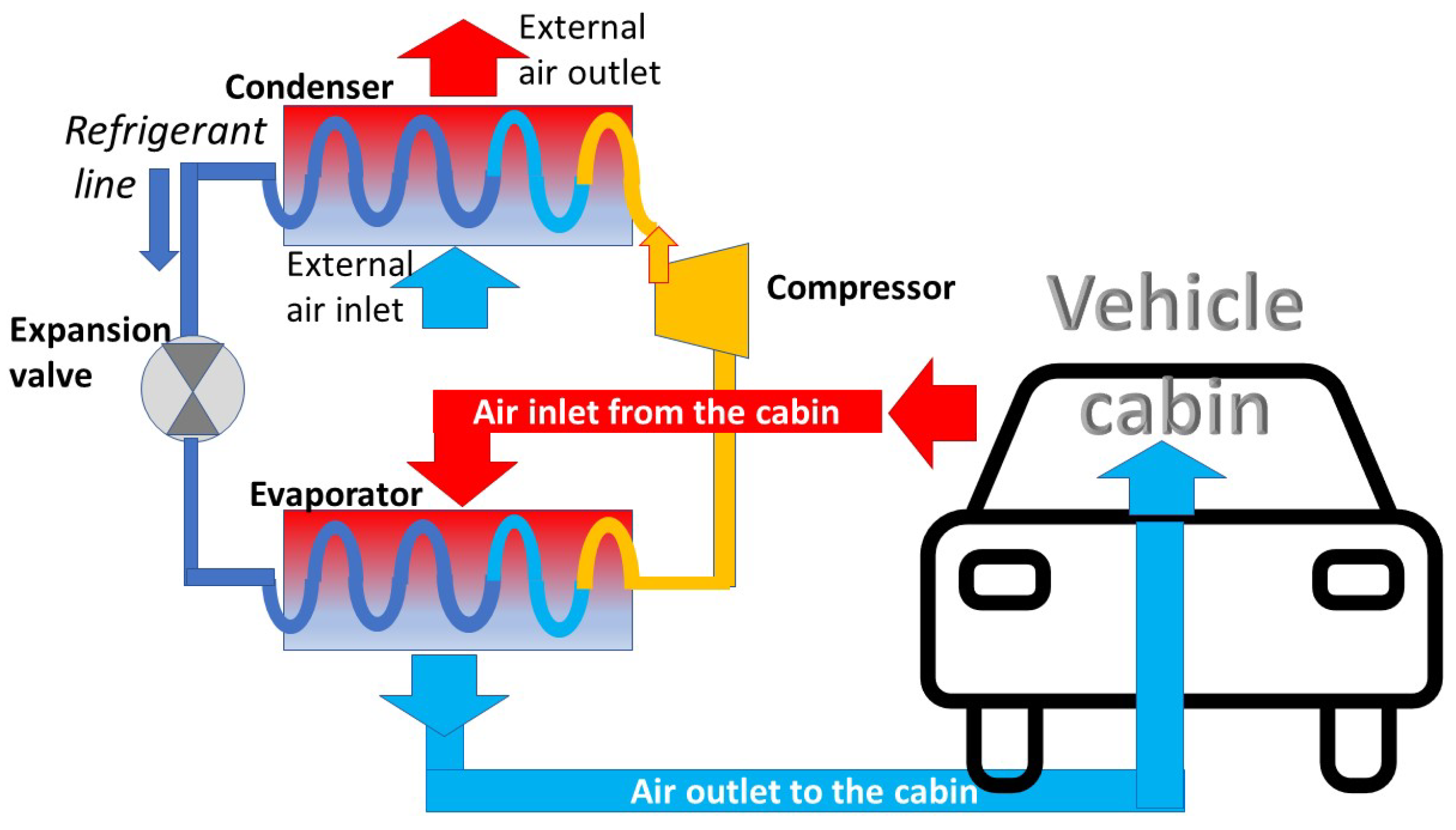
In order to investigate the dynamic behavior of the thermal conditions inside the vehicle cabin, a numerical model of the HVAC system in combination with the vehicle cabin was created within the Simulink environment. In particular, the developed model calculates the temperature inside the vehicle cabin ($T_{cab}$) by the energy balance of external loads (solar radiation, ventilation) and metabolic load [14] with the HVAC system, considering the thermal capacity of the cabin (as shown in Figure 1):

$$\left(m_a{c}_{p,a}\xi \right){\displaystyle \frac{d{T}_{cab}}{dt}}={\dot{Q}}_{rad}\left(t\right)+{\dot{Q}}_{in}\left(t\right)+{\dot{Q}}_{tra}\left(t\right)+{\dot{Q}}_{met}\left(t\right)-{\dot{Q}}_{hvac}\left(t\right)$$

(1)

where ${\dot{m}}_a$ is the mass flow rate of the air blown out from the evaporator, $c_{p,a}$ is the specific heat of air, $\xi$ is a dimensionless parameter that takes into account the thermal inertia of the vehicle, ${\dot{Q}}_{rad}\left(t\right)$ is the thermal load due to the solar radiation, ${\dot{Q}}_{in}\left(t\right)$ is the thermal load due to air infiltration in the cabin, ${\dot{Q}}_{tra}\left(t\right)$ is the transmission load due to the temperature difference between the vehicle and the outer environment, ${\dot{Q}}_{met}\left(t\right)$ is the thermal load due to the presence of people inside the vehicle and ${\dot{Q}}_{hvac}\left(t\right)$ is the cooling power given by the HVAC system. These contributions are variable with time and depend on the boundary conditions, which vary with numerous factors, such as the external weather conditions, the velocity of the vehicle, the number of occupants, etc.

By integrating Equation (1) over a time interval $\Delta t$, it is possible to calculate the evolution in time of the vehicle cabin temperature as follows:

$$T_{cab}\left(t\right)={\displaystyle \frac{1}{m_a{c}_{p,a}\xi }}{\int }_0^{\Delta t}({\dot{Q}}_{rad}\left(t\right)+{\dot{Q}}_{in}\left(t\right)+{\dot{Q}}_{tra}\left(t\right)+{\dot{Q}}_{met}\left(t\right)-{\dot{Q}}_{hvac}\left(t\right))dt$$

(2)

To calculate the temperature evolution of the vehicle cabin, two interconnected Simulink block models were developed, the HVAC model and the vehicle cabin model, which interact with each other. The main blocks of the HVAC system and the mathematical models chosen to simulate the single devices are detailed in the following sections.

2.1. The HVAC Model

The HVAC system consists of four main subsystems: the evaporator, the compressor, the condenser and the expansion valve. Each subsystem is connected to the previous and subsequent subsystems through the main physical properties of the refrigerant fluid: the enthalpy and pressure of the refrigerant fluid and its mass flow rate. The schematic of the connections between the four devices and the heat transfer processes in the evaporator and condenser is shown in Figure 2. In this work, we consider the steady rotational speed of the compressor. Therefore, the volumetric flow rate of the refrigerant is constant inside the single loop, and the mass flow rate depends only on the physical properties of the refrigerant at the compressor inlet. The control system is of an off type, controlled by the vehicle cabin temperature set point $T_{sp}$. Defining the deadband [$T_{sp}-\delta T;T_{sp}+\delta T]$, the following rule is adopted:

$$\left\{\begin{array}{c}{T}_{cab}<T_{sp}-\delta T\mathrm{HVAC}\mathrm{is}\mathrm{off}\\ T_{cab}>T_{sp}+\delta T\mathrm{HVAC}\mathrm{is}\mathrm{on}\end{array}\right.$$

(3)

The energy consumption of HVAC can be calculated as the product between the electrical power consumption ($P_{el}$) and its working time ($\Delta t$):

$$E_{el}=P_{el}·\Delta t$$

(4)

The energy balances within the four main components of the HVAC system are described below.

2.1.1. Evaporator

The thermal power balance in the evaporator can be modeled using the following equation:

$${\dot{Q}}_{eva,ref}\left(p_{eva}\right)={\dot{Q}}_{eva,\Delta T_{ml}}\left(p_{eva}\right),$$

(5)

where ${\dot{Q}}_{eva,ref}$ is the thermal power to the refrigerant and ${\dot{Q}}_{eva,\Delta T_{ml}}$ is the thermal power of the air side calculated using the mean logarithmic temperature difference [15]:

$${\dot{Q}}_{eva,ref}={\dot{m}}_{ref}(h_{ref,out}-h_{ref,in}),$$

(6)

and

$${\dot{Q}}_{eva,\Delta T_{ml}}=f_{eva}{\left(UA\right)}_{eva}\Delta T_{ml}.$$

(7)

In Equation (6), ${\dot{m}}_{ref}$ is the refrigerant mass flow rate, while $h_{ref,out}$ and $h_{ref,in}$ are the enthalpies of the refrigerant fluid, respectively, at the inlet and outlet of the evaporator. In Equation (7), $f_{eva}$ is a correction factor which depends on the evaporator typology, ${\left(UA\right)}_{eva}$ is the product between the global heat transfer coefficient of the evaporator and the heat transfer area (see Equation (11)) and $\Delta T_{ml}$ is the mean logarithmic temperature difference [15]. The mean logarithmic temperature difference requires knowledge of the air and refrigerant temperatures at the inlet and outlet of the evaporator. The air temperature at the evaporator inlet is defined by the ventilation operation condition: indoor temperature set point (in case of recirculation) or external temperature (in case of outdoor air). The air temperature at the outlet of the evaporator ($T_{air,out}$) can be calculated from the following equation:

$${\dot{Q}}_{eva,air}={\dot{Q}}_{eva,air,sen}+{\dot{Q}}_{eva,air,lat}={\dot{m}}_{ref}(h_{ref,out}-h_{ref,in}),$$

(8)

where the sensible and latent heat are obtained by

$${\dot{Q}}_{eva,air,sen}={\displaystyle \frac{{\dot{V}}_{air}{\rho }_{air}}{3600}}{c}_{p,air}(T_{air,in}-T_{air,out}),$$

(9)

and

$${\dot{Q}}_{eva,air,lat}={\displaystyle \frac{{\dot{V}}_{air}{\rho }_{air}}{3600}}r\Delta x,$$

(10)

where r is the water latent heat of vaporization (2430 kJ/kg [16]) and $\Delta x$ is the air humidity difference between inlet and outlet air flow.

The evaporator model is the most complex component in the air conditioning system. This block allows calculation of the thermal load due to refrigerant evaporation, evaluation of the evaporating pressure and change in the physical properties of the refrigerant. The input data are the physical state of the refrigerant (the pressure of the refrigerant fluid is then updated inside the evaporator element), the temperature inside the vehicle at the last iteration, the set-point temperature ($T_{sp}$), the air flow rate and the geometry of the evaporator (or at least its global heat transfer coefficient, $U_{eva}$). In our case, the selected evaporator is made up of flat tubes made of louvered finned microchannels. If the global heat transfer coefficient is not known in advance, it is possible to calculate it from knowledge of the evaporator geometry and the heat transfer mechanism. Then, due to the high conductivity and small thickness of the tubes, the expression of ${\left(UA\right)}_{eva}$ can be simplified as follows [15]:

$${\left(UA\right)}_{eva}={\displaystyle \frac{1}{\frac{1}{h_{ref,eva{A}_{e,i}}}+\frac{1}{h_{air,eva}{A}_{e,o}}}},$$

(11)

where $h_{ref,eva}$ and $h_{air,eva}$ are the heat transfer coefficients on the refrigerant and air side, respectively, while $A_{e,i}$ and $A_{e,o}$ are, respectively, the inner and outer surfaces of the evaporator. Several correlations proposed in the literature were tested for the determination of the heat transfer coefficient on the refrigerant side, $h_{ref,eva}$ [17,18]. As suggested by Zhao et al. (2012) [17], among the several tested correlations, the correlation proposed by Kandlikar and Steinke (2003) [19] was chosen.

$$h_{ref,eva}=max(h_{nbd},h_{cbd}),$$

(12)

where $h_{nbd}$ and $h_{cbd}$ are the flow boiling heat transfer coefficients for nucleate boiling dominance and convective boiling dominance, respectively [19,20]:

$$h_{nbd}=0.6683{\mathrm{Co}}^{-0.2}{(1-x)}^{0.8}{f}_2\left({\mathrm{Fr}}_L\right)h_{L,e}+1058{\mathrm{Bo}}^{0.7}{(1-x)}^{0.8}{F}_{fl}{h}_{L,e}$$

(13)

and

$$h_{cbd}=1.136{\mathrm{Co}}^{-0.9}{(1-x)}^{0.8}{f}_2\left({\mathrm{Fr}}_l\right)h_{l,e}+667.2{\mathrm{Bo}}^{0.7}{(1-x)}^{0.8}{F}_{fl}{h}_{l,e}$$

(14)

where $h_{l,e}$ is the heat transfer coefficient, evaluated considering the refrigerant fluid in the liquid phase. As reported by Kandlikar and Steinke (2003) [19], it can be calculated as follows [21,22,23]:

$$h_{l,e}={\displaystyle \frac{{\mathrm{Re}}_l{Pr}_l(f/2)(k_l/D_h)}{1+12.7{({Pr}_l^{(2/3)}-1(f/2))}^{0.5}}}for{10}^4\le {\mathrm{Re}}_l\le {10}^6$$

(15)

and

$$h_{L,e}={\displaystyle \frac{({\mathrm{Re}}_L-1000){Pr}_l(f/2)(k_l/D_h)}{1+12.7{({Pr}_L^{(2/3)}-1(f/2))}^{0.5}}}for1600\le {\mathrm{Re}}_l\le {10}^4$$

(16)

and

$$h_{L,e}=\mathrm{Nu}{\displaystyle \frac{k_l}{D_h}}for{\mathrm{Re}}_l\le 1600$$

(17)

where ${Pr}_l$ and ${\mathrm{Re}}_l$ are the dimensionless Prandtl and Reynolds numbers considering the refrigerant in the liquid phase, f is the friction function ($f={[1.58ln\left({\mathrm{Re}}_l\right)-3.28]}^{-2}$), $k_l$ is the thermal conductivity of the refrigerant in the liquid phase and $D_h$ is the hydraulic diameter of the microchannels. In Equation (17), $\mathrm{Nu}$ is the Nusselt number, which depends on the geometry of the channels and the boundary conditions acting on the walls of the evaporator.

In Equations (13) and (14), x is the vapor quality of the mixture, $f_2\left({\mathrm{Fr}}_l\right)$ is a correction factor based on the Froude number (equal to 1 for microchannels [19]) and $F_{fl}$ is a parameter which depends on the typology of the adopted refrigerant. In the case of R134a, $F_{fl}$ is equal to 1.63 [19]. The two dimensionless parameters which appear in Equations (13) and (14) are the Convection number ($\mathrm{Co}$) and the Boiling number ($\mathrm{Bo}$), defined as

$$\mathrm{Co}={\left({\displaystyle \frac{{\rho }_v}{{\rho }_l}}\right)}^{0.5}{\left({\displaystyle \frac{1-x}{x}}\right)}^{0.8}\mathrm{Bo}={\displaystyle \frac{q}{G{h}_{\overline{ls}}}}$$

(18)

where ${\rho }_v$ and ${\rho }_l$ are the densities of the refrigerant in the gas and liquid phases, q is the heat flux over the evaporator walls, G expresses the ratio between the mass flow rate of the refrigerant fluid and the cross-sectional area of the microchannels and $h_{\overline{ls}}$ is the maximum latent heat of vaporization for a given pressure. The heat transfer coefficient on the refrigerant side is evaluated from the evaporating pressure and the refrigerant mass flow rate. The air-side heat transfer coefficient $h_{air,eva}$ is usually expressed through the Colburn factor j that expresses the Nusselt number as a function of the Reynolds and Prandtl dimensionless numbers:

$${\mathrm{Nu}}_{air,eva}=j{\mathrm{Re}}_{air}\underset{air}{\overset{(1/3)}{Pr}}.$$

(19)

Hence, the air-side heat transfer coefficient $h_{air,eva}$ can be expressed as follows:

$$h_{air,eva}=j_{eva}{\displaystyle \frac{{\rho }_{air}{v}_{air}{k}_{air}}{{\mu }_{air}}}{\left({\displaystyle \frac{{\mu }_{air}{c}_{p,air}}{k_{air}}}\right)}^{(1/3)}$$

(20)

where ${\rho }_{air}$, $v_{air}$, $k_{air}$, ${\mu }_{air}$ and $c_{p,air}$ are the density, velocity, thermal conductivity and specific heat of the air. In agreement with the chosen evaporator, the Colburn factor j can be calculated using the correlation proposed by Chang and Wang (1997) [24]:

$$j_{eva}=R{e}_{Lp}^{-0.19}{\left({\displaystyle \frac{\theta }{90}}\right)}^{0.27}{\left({\displaystyle \frac{F_p}{L_p}}\right)}^{-0.14}{\left({\displaystyle \frac{F_l}{L_p}}\right)}^{-0.29}{\left({\displaystyle \frac{T_d}{L_p}}\right)}^{-0.23}{\left({\displaystyle \frac{L_l}{L_p}}\right)}^{0.68}{\left({\displaystyle \frac{T_p}{L_p}}\right)}^{-0.28}{\left({\displaystyle \frac{{\delta }_f}{L_p}}\right)}^{-0.05},$$

(21)

where ${\mathrm{Re}}_{Lp}$ is the Reynolds number based on the louver spacing ($L_p$), $\theta$ is the louver angle, $F_p$ is the fin spacing, $F_l$ is the fin length, $T_d$ is the main diameter of the tube (the correlation is valid for flat tubes), $L_l$ is the louver length, $T_p$ is the tube spacing and ${\delta }_f$ is the fin thickness. A list of typical parameters for commercial heat exchangers can be found in the work of Chang and Wang (1997) [24]. As the refrigerant side heat transfer coefficient, the air side heat transfer coefficient also changes during the simulation because it depends both on the volumetric flow rate and on the temperature of the air entering the evaporator. Once the pressure of the refrigerant fluid has been defined inside the evaporator, it is then possible to determine the physical quantities of the fluid at the inlet of the compressor. In doing so, it is important to keep in mind that the refrigerant fluid enters the compressor in a superheated vapor state.

2.1.2. Compressor

The compressor model, which is in our case a scroll compressor, calculates for each iteration the refrigerant mass flow rate. The input data are the rotational speed of the compressor $V_{r,comp}$ and its discharge capacity ($DC$), while the density of the refrigerant ${\rho }_{ref}$ is obtained from the physical state of the refrigerant fluid given by the evaporator outlet. The mass flow rate of the refrigerant fluid ${\dot{m}}_{ref}$ can be calculated as follows:

$${\dot{m}}_{ref}={\dot{V}}_{ref}·{\rho }_{ref},$$

(22)

where

$${\dot{V}}_{ref}={\displaystyle \frac{DC·V_{r,comp}}{60·{10}^6}}.$$

(23)

The condensing pressure ($p_{cond}$) is defined by the condensing temperature of the refrigerant, which is defined by adding to the external air temperature a pinch point temperature difference. The compression ratio is defined by the ratio between the condensing pressure and the evaporating pressure. The compressor outputs include the physical state of the refrigerant at the component outlet. In this case, the enthalpy of the refrigerant fluid is determined using the isentropic efficiency of the compressor. Finally, the energy consumption of the compressor is evaluated according to Equation (4).

2.1.3. Condenser

In addition to updating the physical states of the refrigerant fluid, the condenser element calculates the heat exchange between the refrigerant fluid and the external air. The thermal power balance in the condenser can be modeled using the following equation:

$${\dot{Q}}_{c,\Delta T_{ml}}={\dot{Q}}_{c,ref},$$

(24)

where ${\dot{Q}}_{c,\Delta T_{ml}}$ and ${\dot{Q}}_{c,ref}$ are, respectively, the thermal power determined by using the mean logarithmic temperature difference and the thermal power determined from the energy balance on the refrigerant fluid side:

$${\dot{Q}}_{c,\Delta T_{ml}}=f_c{\left(UA\right)}_{cond}\Delta T_{ml},$$

(25)

and

$${\dot{Q}}_{c,ref}={\dot{m}}_{ref}(h_{ref,vs}\left(p_{cond}\right)-h_{ref,lsc}\left(p_{cond}\right)).$$

(26)

Similar to Equation (7), in Equation (25), $f_c$ is a correction factor which depends on the compressor typology [15], ${\left(UA\right)}_{cond}$ is the global heat transfer coefficient of the compressor multiplied by the heat transfer area of the condenser and $\Delta T_{ml}$ is the mean logarithmic temperature difference. In Equation (26), $h_{ref,vs}\left(p_{cond}\right)$ is the enthalpy of the refrigerant fluid in the state of superheated vapor at the inlet of the condenser and $h_{ref,lsc}\left(p_{cond}\right)$ is the enthalpy of the refrigerant fluid in the state of subcooled liquid at the outlet of the condenser. Hence, after solving Equation (25), it is possible to use Equation (26) in order to determine the temperature of the condensed refrigerant fluid. In addition, in this case, if the global heat transfer coefficient ($U_c$) is not known in advance, it is possible to calculate it as follows:

$${\left(UA\right)}_{cond}={\displaystyle \frac{1}{\frac{1}{\overline{h_{ref,c}}{A}_{tot,c,i}}+\frac{1}{h_{air,c}{A}_{c,o}}}}.$$

(27)

In Equation (27), $\overline{h_{ref,c}}$ is the mean heat transfer coefficient of the refrigerant side (see Equation (28)) and is multiplied by the total inner heat transfer surface of the condenser ($A_{tot,c,i}$), and $h_{air,c}$ is the air-side heat transfer coefficient, which is multiplied by the outer heat transfer surface of the condenser ($A_{c,o}$).

$$\overline{h_{ref,c}}=h_{r,c}·\left({\displaystyle \frac{A_{tot,c,i}-A_{vs,c,i}}{A_{tot,c,i}}}\right)+h_{vs,c}·A_{vs,c,i}$$

(28)

where $h_{r,c}$ and $h_{vs,c}$ are the heat transfer coefficients of the refrigerant during its condensing phase and during its cooling from the superheated vapor state to the saturated vapor state. $A_{vs,c,i}$ is the portion of the condenser heat transfer coefficient in the inner area devoted to cooling of the refrigerant from the superheated vapor state to the saturated vapor state. The heat transfer coefficient $h_{vs,c}$ can be calculated from the Nusselt number determined by the Dittus–Boelter correlation for the cooling of superheated vapor [15], while the heat transfer coefficient $h_{r,c}$ can be calculated using the correlation of Cavallini et al. (2006) [25], reported in the following equation.

$$\left\{\begin{array}{c}{h}_{r,c}=h_A\mathrm{for}{J}_G>J_G^T\\ h_{r,c}=h_D\mathrm{for}{J}_G\le J_G^T\end{array}\right.$$

(29)

where

$$J_G={\displaystyle \frac{xG}{{\left[g{D}_h{\rho }_v({\rho }_l-{\rho }_v)\right]}^{0.5}}}$$

(30)

and

$$J_G^T={\left\{{\left[{\displaystyle \frac{7.5}{\left(4.3X_{tt}^{1.111}+1\right)}}\right]}^{-3}+C_T^{-3}\right\}}^{-(1/3)}$$

(31)

where $J_G$ is the modified Froude number and is used as the dimensionless gas velocity, while $J_G^T$ is a threshold parameter involved in determining the transition between the regime in which the heat transfer coefficient depends on the difference between the saturation temperature and the inner wall temperature of the tube and the regime in which it does not depend on this value [25]. In Equation (31), $X_{tt}$ is the Martinelli parameter and $C_T$ is a parameter that takes into account whether the refrigerant fluid is a hydrocarbon ($C_T$ = 1.6) or not ($C_T$ = 2.6) [25]. The heat transfer coefficient of the refrigerant during condensation is calculated as follows:

$$h_A=h_{L,c}\left[1+1.128x^{0.817}{\left({\displaystyle \frac{{\rho }_l}{{\rho }_v}}\right)}^{0.3685}{\left({\displaystyle \frac{{\mu }_l}{{\mu }_v}}\right)}^{0.2363}{\left(1-{\displaystyle \frac{{\mu }_v}{{\mu }_l}}\right)}^{2.144}P{r}_L^{-0.1}\right]$$

(32)

and

$$h_D=\left[h_A{\left({\displaystyle \frac{J_G^T}{J_G}}\right)}^{0.8}-h_{st}\right]\left({\displaystyle \frac{J_G}{J_G^T}}\right)+h_{st}$$

(33)

where $h_{L,c}$ and $h_{st}$ can be determined using the following Equations [25]:

$$h_{l,c}=0.023{\mathrm{Re}}_l^{0.8}\underset{l}{\overset{0.4}{Pr}}\left({\displaystyle \frac{k_L}{D_h}}\right)$$

(34)

and

$$h_{st}=0.725{\left[1+0.741{\left({\displaystyle \frac{1-x}{x}}\right)}^{0.3321}\right]}^{-1}{\left[{\displaystyle \frac{k_L^3{\rho }_l({\rho }_l-{\rho }_g)g{h}_{\overline{LS}}}{{\mu }_l{D}_h\Delta T}}\right]}^{0.25}+\left(1-x^{0.087}\right)h_{L,c}$$

(35)

In Equation (35), $h_{\overline{LS}}$ is the latent heat of condensation and $\Delta T$ is the temperature difference between the saturation temperature and the inner wall temperature.

2.1.4. Expansion Valve

The expansion valve gives the evaporator pressure ($p_{eva}$) by means of the following equation:

$$p_{eva}=p_{cond}/\beta .$$

(36)

This value is updated inside the evaporator element as explained in Section 2.1.1.

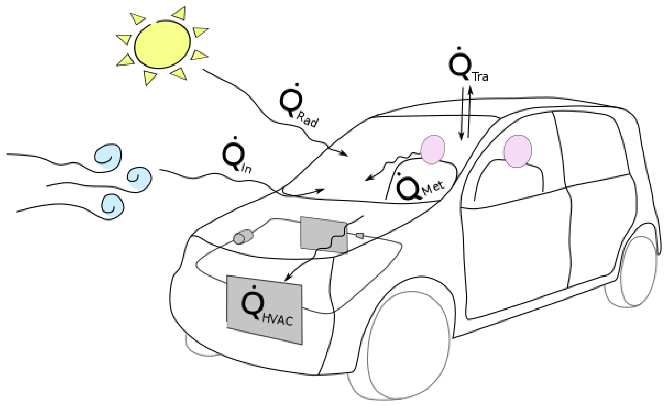
2.2. The Cabin Model

The cabin model interacts with the HVAC model through the temperature inside the vehicle cabin. This model considers all the thermal loads reported in Equation (1). The details of all external loads acting on the vehicle cabin are reported below.

2.2.1. Solar Radiation

The main contribution during summer is the thermal load due to the solar radiation. As also outlined in the Ashrae Fundamentals Handbook (1997) [26], the total solar radiation that affects the vehicle body is composed of the following components:

• Direct solar radiation, depending on the incident angle $\theta$ of the normal solar radiance $I_{dn}$ with respect to the normal of the surface.
• Diffuse sky radiation $I_{diff}$.
• Albedo $I_{alb}$, depending on reflections from the ground and surrounding surfaces.

Hence, the thermal load due to solar radiation can be calculated as follows [14]:

$${\dot{Q}}_{rad}=\sum _s{S}_s\alpha (I_{dn}·cos\left(\theta \right)+I_{diff}+I_{alb}),$$

(37)

where $S_s$ is the vehicle surface and $\alpha$ is the surface absorptivity. In our case, a surface absorptivity equal to 0.2 [27] was assumed for the entire surface of the external vehicle.

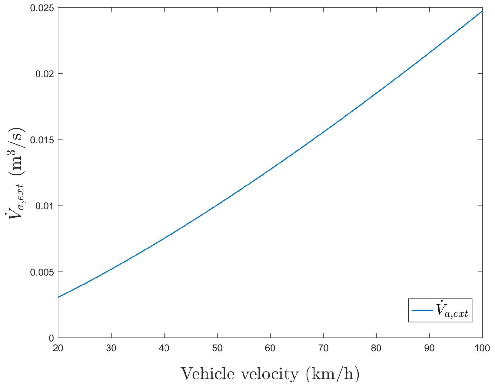
2.2.2. Ventilation and Infiltration

In order to enable proper operation of the HVAC system, windows are considered closed and the air conditioning system works in the air recirculation mode. As the vehicle body is not perfectly sealed, infiltration of external air occurs inside the vehicle cabin as a function of the pressure difference between the internal and external environments. The amount of air entering from the outside was experimentally studied by Fletcher and Saunders (1994) [28] in the case of a stationary vehicle and in the case of a vehicle in movement. The infiltration flow rate can be calculated as follows [28]:

$${\dot{m}}_{a,ext}={\rho }_{air}·{\dot{V}}_{a,ext}={\rho }_{air}·0.1C{\left({\displaystyle \frac{{\rho }_{air}}{2}}\right)}^n{v}^{2n},$$

(38)

where C and n are experimental coefficients and depend both on vehicle typology and operative conditions [28], while v is the speed of the car. Therefore, the thermal load due to infiltration can be expressed as

$${\dot{Q}}_{in}={\dot{m}}_{a,ext}·(h_{a,out}-h_{a,in}).$$

(39)

The specific air enthalpy $h_a$ can be calculated as follows:

$$h_a=T_a{c}_{p,a}+\left(T_a{c}_{p,w}+r\right)x_a,$$

(40)

where $T_a$ is the temperature of the air, $c_{p,a}$ is the specific heat of the air, $c_{p,w}$ is the specific heat of water vapor, r is the latent heat of the vaporization of the water, $x_a$ is the humidity ratio and $\phi$ is the relative humidity. The humidity ratio is a function of saturation pressure $P_{sat}$ as follows:

$$x_a=0.622{\displaystyle \frac{\phi P_{sat}}{101325-\phi P_{sat}}},$$

(41)

where

$$P_{sat}=e^{\left(65.81-{\displaystyle \frac{7066.27}{T_a+273.15}}-5.976ln(T_a+273.15)\right)}.$$

(42)

When the vehicle is not in motion, a volumetric air flow rate equal to 10 ⁻³m³/h is assumed.

2.2.3. Heat Transmission Through the Vehicle Envelope

The thermal load owing to the difference in temperature between the air inside the vehicle and the outer environment can be determined as follows:

$${\dot{Q}}_{tra}=U_{cab}{A}_{cab}(T_{ext}-T_{cab}),$$

(43)

where $U_{cab}$ is the mean global heat transfer coefficient of the vehicle body and $A_{cab}$ is the total outer surface of the car.

2.2.4. Metabolic Load

The metabolic load due to the presence of people inside the vehicle can be evaluated according the ISO 8996 standard [29]:

$${\dot{Q}}_{met}=n_p{\dot{q}}_p{S}_p,$$

(44)

where $n_p$ is the number of people inside the vehicle, ${\dot{q}}_p$ is the thermal load per unit of area of the person and $S_p$ is the standard outer surface of the person. The ISO 8996 International Standard suggests values of thermal load ${\dot{q}}_p$ for different cases, such as people at rest or during car driving.

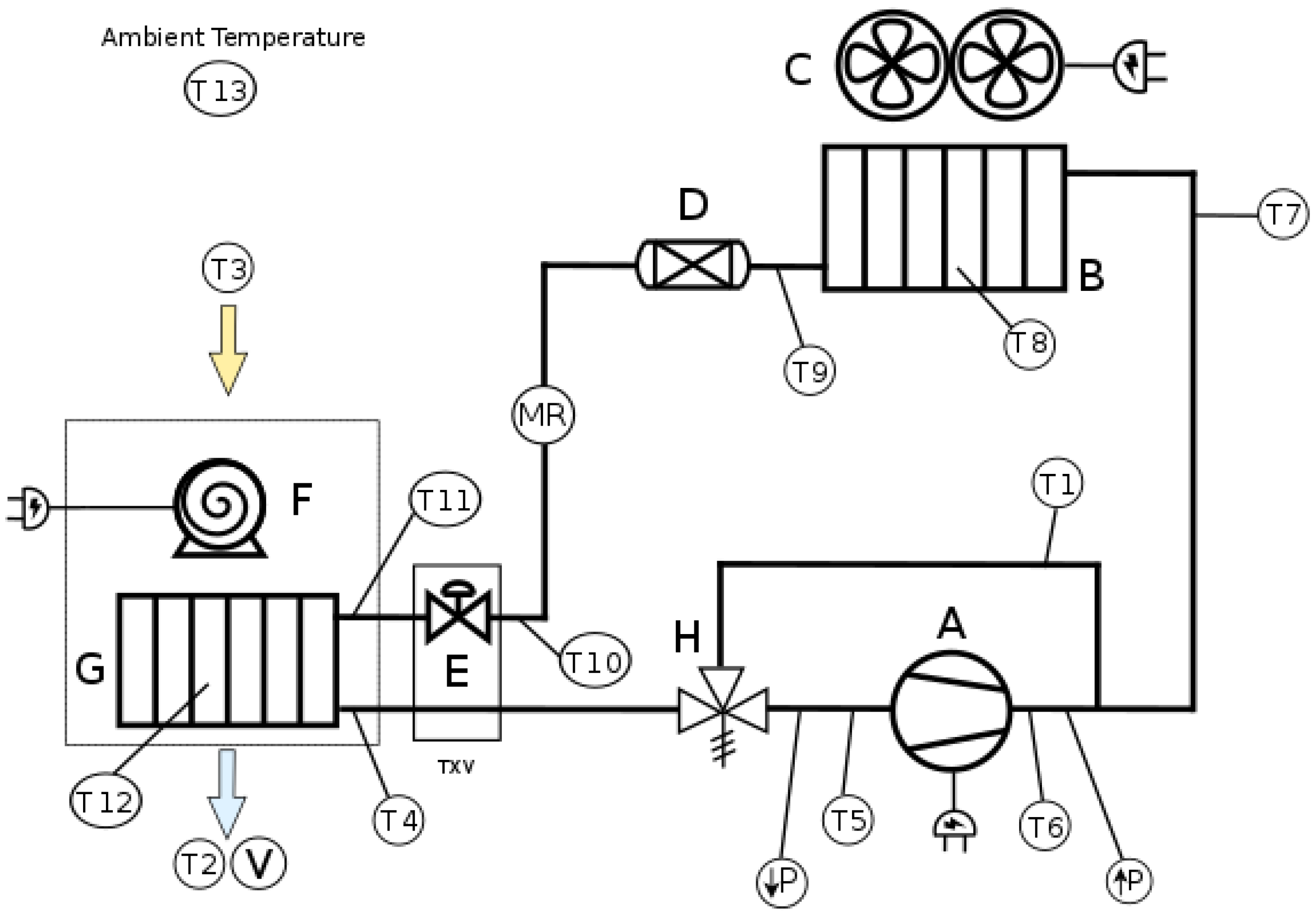
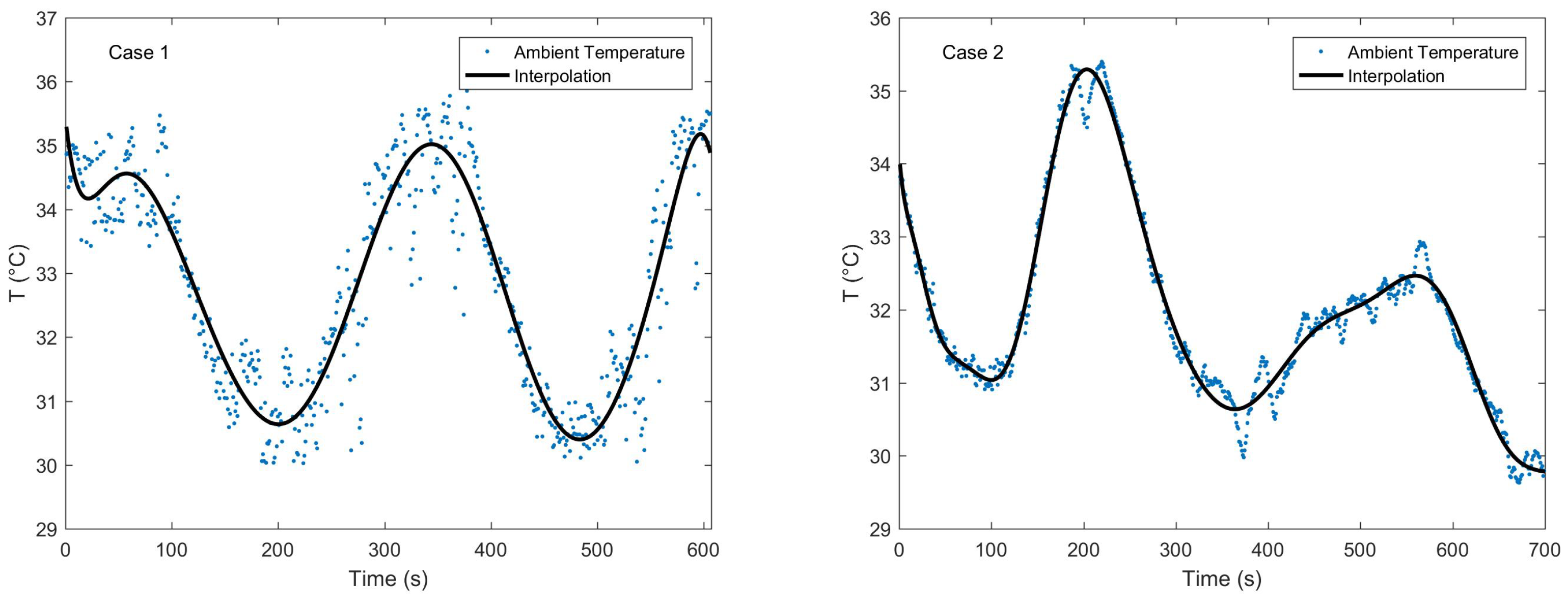
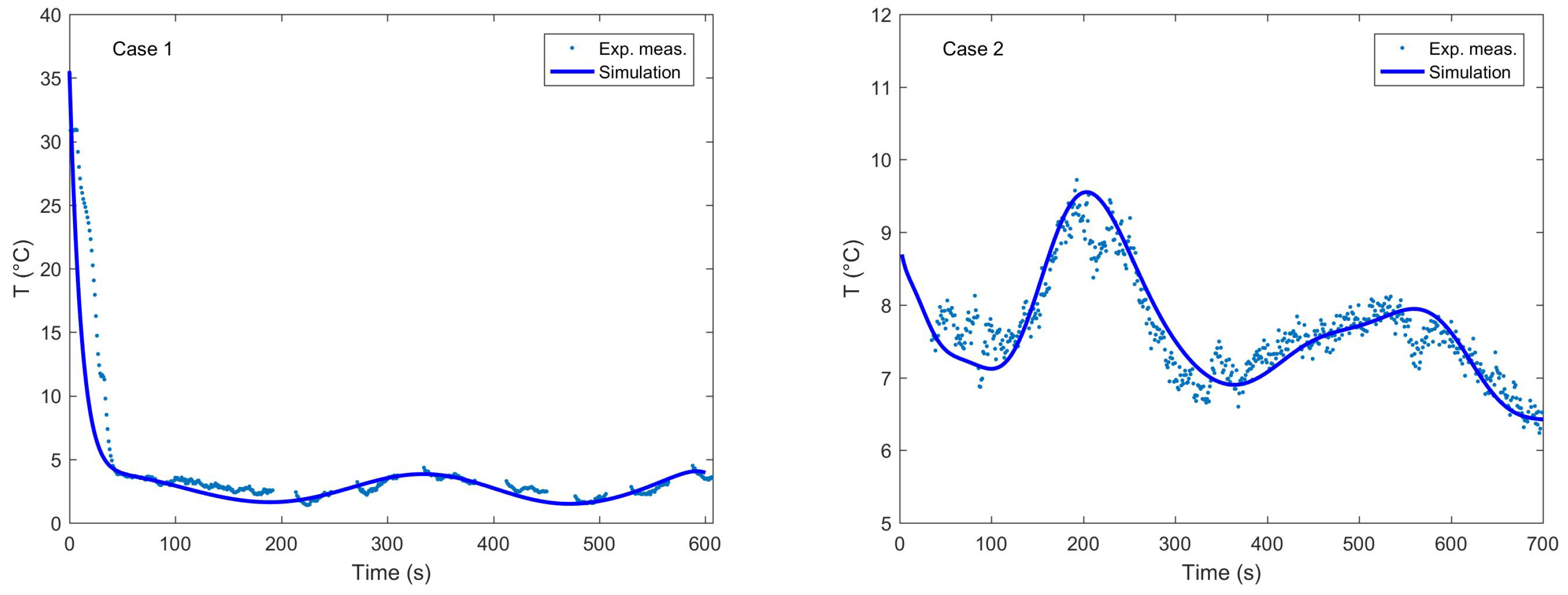
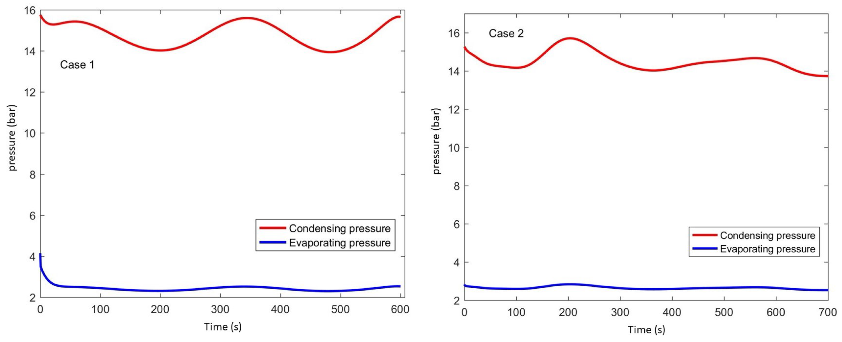
3. Validation of the Model

The model was validated through experimental measurements performed on a real air conditioning system built ad hoc for an internal combustion engine vehicle that was retrofitted to an electric vehicle. The HVAC system is composed of an aluminum evaporator with two rows of 38 parallel flat tubes with a length of 0.11 m and 72 fins each. The internal exchange area is 0.4682 m², while the external exchange area is 1.2 m². The condenser is a finned tube heat exchanger, with an internal exchange area of 0.7297 m² and an external exchange area of 1.8974 m². The compressor is a Benling scroll compressor DM18A8, with a discharge capacity equal to 18 cc/rev and a maximum power of 2 kW. The air temperatures and the refrigerant side temperatures were measured using 13 thermocouples as shown in Figure 3.

All data were acquired by specific software developed on a Labview platform. The temperatures of the refrigerant fluid were acquired by placing the thermocouples on the metallic surface of the corresponding component.

The pressure of the refrigerant fluid was continuously checked using two pressure sensors located before and after the compressor. With this configuration, it was possible to evaluate the minimum and maximum pressures of the refrigerant fluid within the system. The mass flow rate of the refrigerant fluid was measured using a Coriolis flow and density meter (Emerson Micro Motion R025) installed along the branch connecting the receiver dryer after the condenser outlet with the inlet of the expansion valve (MR in Figure 3). This position allows a correct reading of the refrigerant mass flow (the refrigerant fluid is in the liquid phase) and allows the measurement of the actual mass flow entering the expansion valve. The volumetric air flow rate was measured for different fan velocities using an integral anemometer (KIMO LV130) placed in correspondence to the air flow at the evaporator outlet (V in Figure 3).

Table 1. Table of experimental uncertainties.

Description	Uncertainty
T-type thermocouples	±0.5 °C
Low-pressure gauge	±0.2 bar
High-pressure gauge	±0.5 bar
Refrigerant mass flow rate	±0.5% of reading
Volumetric air flow rate	±3% of reading

summarizes the uncertainties of the measuring devices used for the experiments. The HVAC system, together with the related measurement instrumentation, were placed inside a remotely controlled climatic chamber. All thermal loads described in Section 2.2 were considered null to validate the HVAC system independently from the vehicle cabin model.

Test Conditions

Different tests were carried out by changing the system settings (such as fan speed) and repeated for different temperatures of the climatic room. Among the different test conditions, two particular cases were chosen for the validation of the model. The first dealt with the air conditioning system start procedure: in this case, the HVAC system was turned off for several hours inside the climatic room, which had an average temperature of 32.5 °C. In this way, all the system components were at the same temperature as the surrounding environment. The system was turned on, with an air flow rate through the evaporator equal to 160 m³/h. The second case started just at the end of the first case, with an air flow rate of 240 m³/h. The temperature trends inside the climatic room during the two tests are reported in Figure 4.

The blue points are the experimental measurements, while the black line is the interpolation. The wide range of temperature variation within the climatic room (30–35 °C) was chosen as an example of real variability in the atmospheric condition. The interpolating function was used as the ambient temperature input in the Simulink model. The measured relative humidity was 0.31 for the first case and 0.26 for the second case. The model developed allows us to simulate the continuous behavior of several quantities, such as the physical states of the refrigerant fluid and its mass flow rate, the mean condensing and evaporating pressure, the different powers related to the air conditioning system and the temperature and volumetric flow rate through the evaporator. Among these different variables, the most relevant to take into account for the model validation is the air temperature at the evaporator outlet. Hence, the comparison between the temperature measurements of the air exiting the evaporator and the corresponding simulated one is shown in Figure 5.

In both figures, the dots represent the experimental measurements, while the continuous line represents the simulated trend. As is visible from the pictures, there is good agreement between the simulation results and the experimental measurements in both the start-up condition (case 1) and the maximum load condition (case 2). Figure 5 (right) shows that the variation in the air temperature at the exit of the evaporator is related to fluctuations in the air temperature at the exit (Figure 4 (right)). The time evolution obtained for the evaporating and condensing pressures is shown in Figure 6.

The total pressure drop in the evaporator was set at 0.36 bar [17], while the pressure drop in the condenser was set at 0.6 bar.

Table 2. Comparison between mean simulated and measured pressures (bar).

Description	Case	Simulation	Measurements
High pressure	1	14.8	15.5 ± 0.5
Low pressure	1	2.1	2.0 ± 0.2
High pressure	2	14.4	15.0 ± 0.5
Low pressure	2	2.3	2.0 ± 0.2

shows the comparison between the mean simulated pressure values and the related measured ones. The table shows that the simulated data agree very well with the experimental measurements.

Validation was performed for numerous boundary conditions, combining the room temperature in the range (30–50 ° C) and the humidity in the range (30–60%). The simulation results consistently deviated from the experimental measurements by values below 10%. Therefore, the proposed model can be considered validated in a wide range of climatic conditions.

4. Results and Discussion

In this section, the energy consumption of the HVAC system is analyzed for two representative driving conditions. In the first, there is only one person in the car, driving at a constant speed for 40 min during a hot summer day. In the second, a regulated driving cycle (ECE 15 driving cycle [13]) is repeated for one hour. In the first driving condition, the case in which the driver enters the hot car and starts driving immediately is compared with the case where the car has undergone a precooling phase.

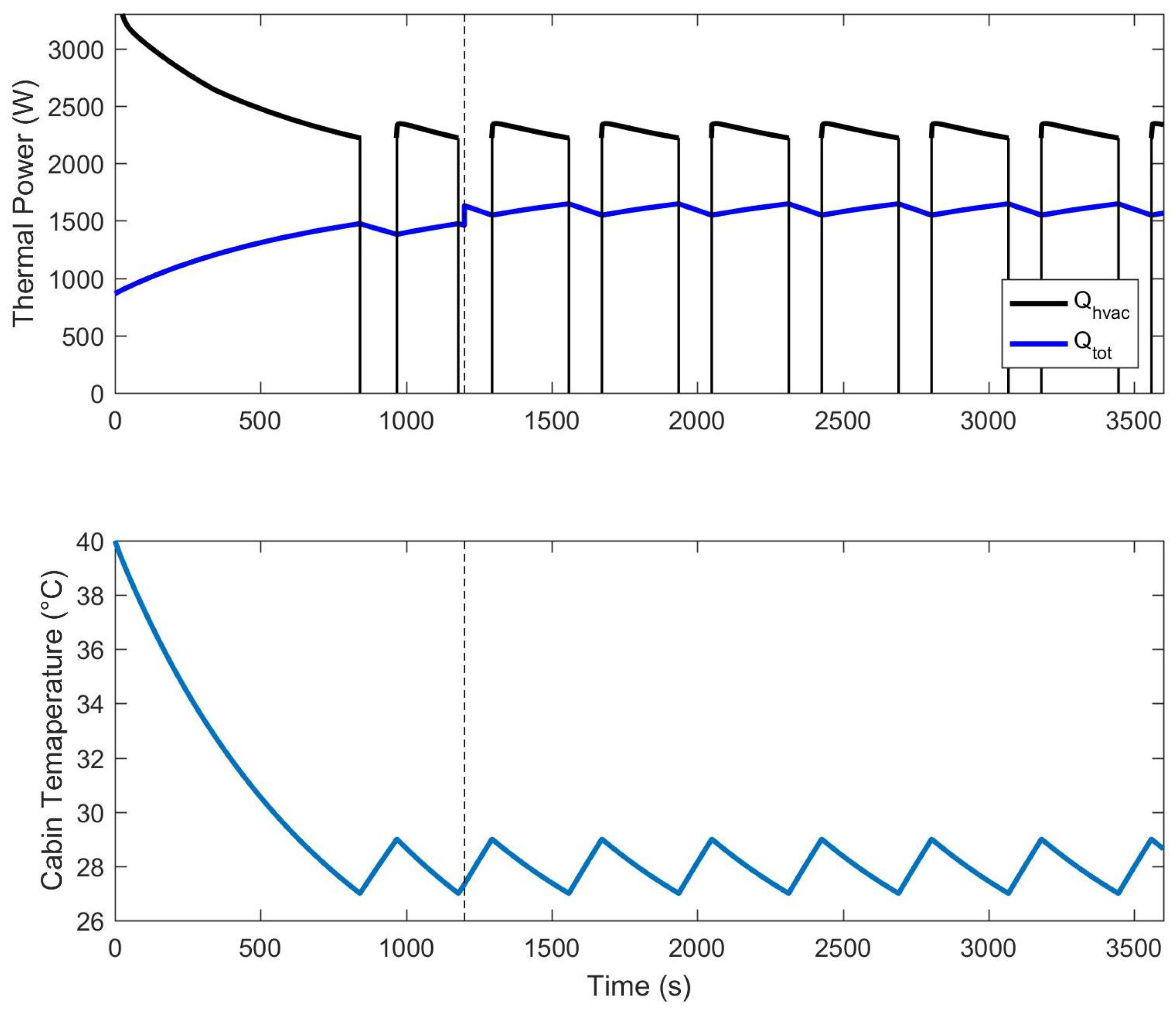
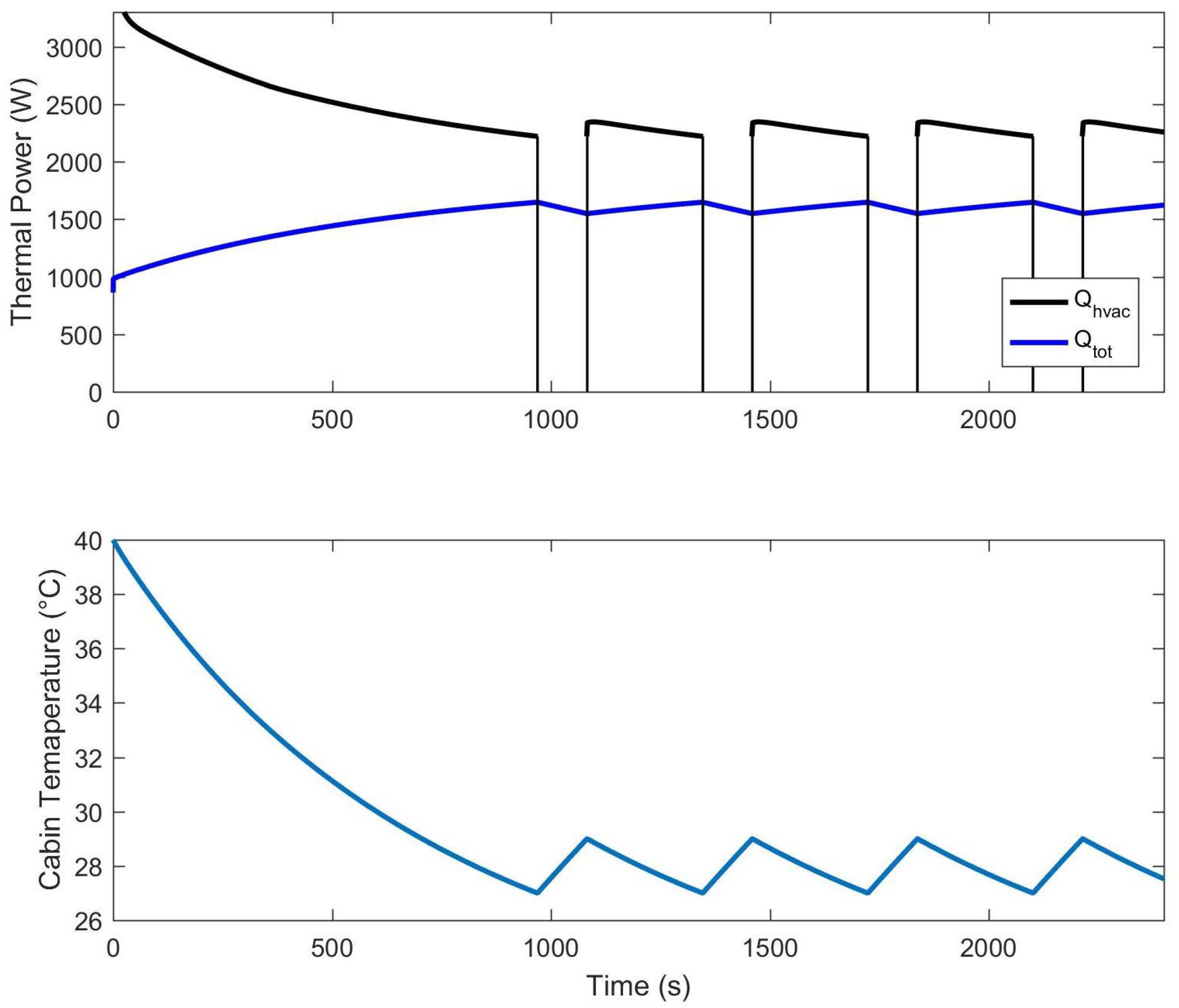
4.1. Constant Speed Driving Condition and the Influence of Precooling Phase

The adoption of a precooling phase gives advantages in terms of comfort conditions inside the vehicle together with a lower battery electric consumption during the driving. In order to evaluate the effective advantages, the cases with and without the precooling phase are compared in this section.

Table 3. Common conditions imposed in both cases.

Imposed Condition		Values
Outdoor temperature	$T_{ext}$	35 °C
Initial inner temperature	$T_{cab}$	40 °C
Relative humidity	${\phi }_{ext}$	35%
Solar thermal load	${\dot{Q}}_{rad}$	1100 W
Passenger number		1

shows the common conditions imposed as input in both cases, while

Table 4. Different settings between the two cases.

With Precooling
Simulation time	3600 s
Average vehicle velocity (t < $t_0$ )	0 km/h
Average vehicle velocity (t > $t_0$ )	20 km/h
Without Precooling
Simulation time	2400 s
Average vehicle velocity	20 km/h

shows the different assumptions made in order to compare the two different solutions. In the first case, the car undergoes a precooling phase from 0 to $t_0$ = 1200 s with the HVAC system on, and a second period from $t_0$ to $t_1=3600$ s when the user is inside the car and drives at an average velocity of 20 km/h. In the second case, the car is not cooled before the user arrival, and the simulation starts when the user enters the car. In order to compare this second case with the previous one, the second case ends at 2400 s and the average velocity of the vehicle is equal to 20 km/h. In both simulations, the initial temperature inside the vehicle cabin is 40 °C.

The results are shown in Figure 7 for the case with the precooling phase and in Figure 8 for the case without. In the figures, ${\dot{Q}}_{hvac}$ represents the thermal power exchanged in the evaporator. From this variable, we determine the coefficient of performance (COP) of the cycle, which is variable, with a maximum value of 3.6.

Figure 7 shows that once the user enters the vehicle (dotted line), the temperature inside the cabin has already reached the comfort set point. More precisely, after almost 14 min, $T_{cab}$ reached the set-point value ($T_{sp}$) and the system started the on–off cycle. This means that for all of the driving period, the HVAC system works only to keep the temperature inside the vehicle cabin at the comfort temperature. On the contrary, without the employment of the precooling phase, when the user enters the vehicle, the temperature inside the vehicle is equal to the maximum temperature (i.e., 40 °C) and the HVAC system must continue to work until it reaches the comfort temperature before starting the on–off cycle (as shown by Figure 8).

Regarding the energy consumption of the batteries ($E_{el,batt}$), the analysis can be made as follows. In the case of the precooling phase, the energy absorbed from the batteries during the driving period can be calculated as the integral of the power absorbed from the compressor ($P_{el}$) over the time interval $\Delta t=t_1-t_0$:

$$E_{el,batt}={\int }_{t_0}^{t_1}\delta \left(t\right)P_{el}dt$$

(45)

where $\delta \left(t\right)$ is a function equal to 1 when the system is “on” and equal to 0 when the system is “off”. In our specific case, Equation (45) gives a value of 0.65 kWh. Similarly, the energy consumption of the batteries during the driving period due to the HVAC system without the adoption of the precooling phase can be calculated by using Equation (45) and changing the time interval to [0–2400 s]. In this case, Equation (45) gives a value of 0.78 kWh, which is about 16% higher than the case with precooling. However, the adoption of the precooling phase requires additional energy consumption during the battery charging, which in this case is 0.42 kWh; therefore, the total amount of energy requested by the HVAC system is 1.08 kWh. In reducing the precooling time to 840 s instead of 1200 s, the total amount of energy required for vehicle cooling (840 s of precooling and 2400 s of driving) decreases to 0.99 kWh, saving about 8.6% of the energy for battery charging. Then, the adoption of the precooling phase reduces the energy consumption during the driving period and increases the overall energy consumption. Therefore, with the model developed, it is possible to predict whether the adoption of the precooling phase gives advantages in terms of energy consumption and comfort conditions.

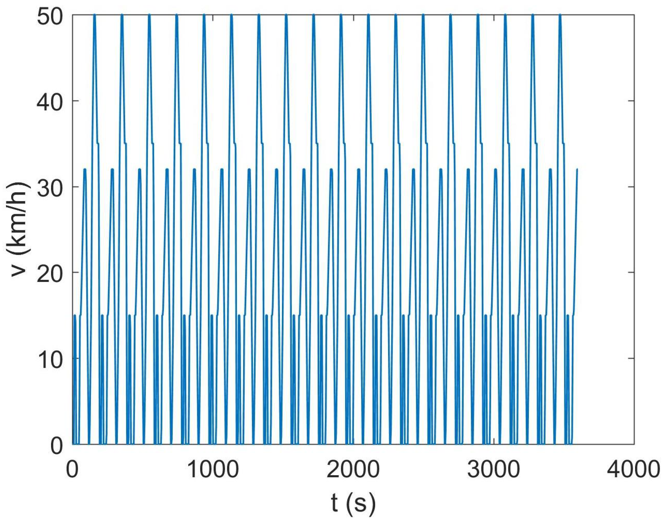
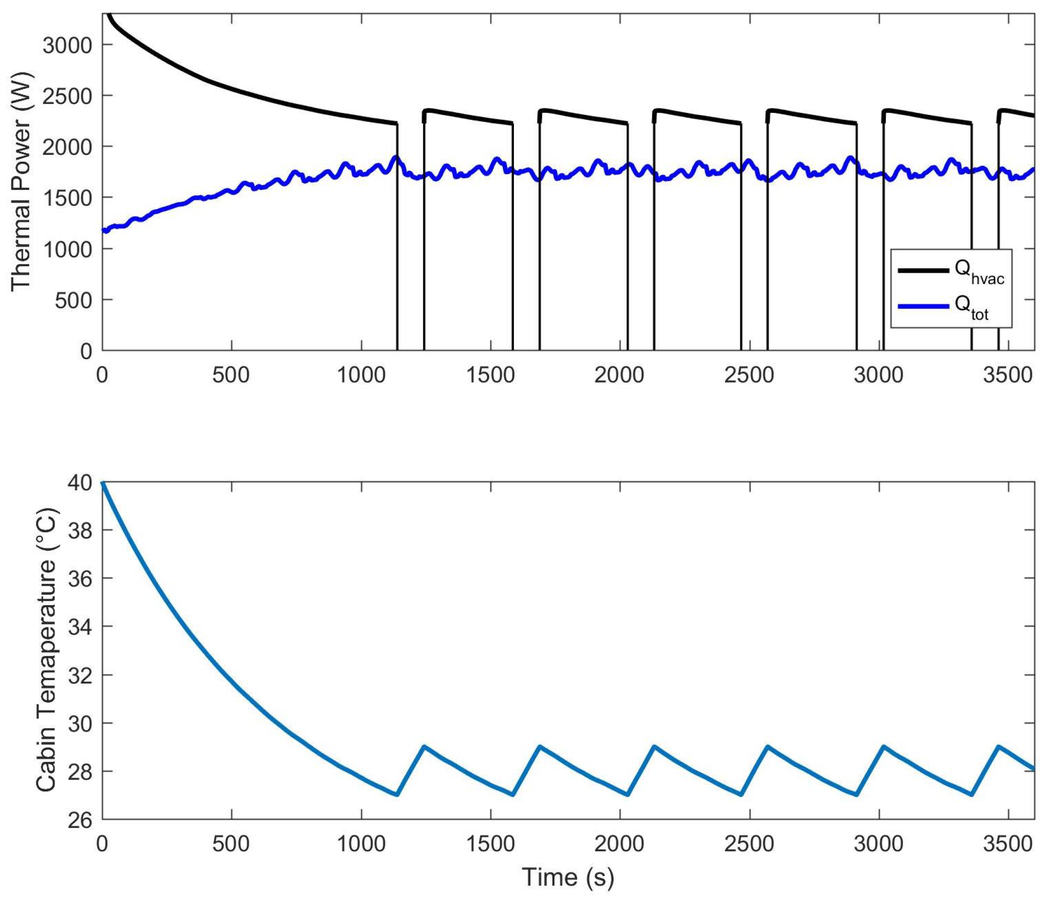
4.2. ECE 15 Driving Cycle

The ECE 15 driving cycle simulates urban mobility where the maximum speed of the vehicle is limited to 50 km/h, while its average speed in the cycle is equal to 18.4 km/h [13]. The powertrain of the vehicle is made up of lithium ion batteries having an electrical capacity 320 Ah with a discharge voltage of 50 V. The vehicle parameters, including the state of charge (SOC) of the batteries as well as the comfort conditions inside the cabin, were simulated with and without the use of the HVAC system. The main input conditions imposed in this case are reported in

Table 5. Main input conditions imposed in the ECE 15 case.

Imposed Condition		Values
Simulation time		3600 s
Outdoor temperature	$T_{ext}$	35 °C
Initial inner temperature	$T_{cab}$	40 °C
Relative humidity	${\phi }_{ext}$	35%
Solar thermal load	${\dot{Q}}_{rad}$	1100 W
Passenger number		2
Set-point temperature	$T_{SP}$	28 °C
Total distance covered		19.8 km

, while the vehicle velocity is shown in Figure 9.

The thermal load due to solar radiation ${\dot{Q}}_{rad}$ was taken as constant during the hourly simulation, and the metabolic load ${\dot{Q}}_{met}$ depended on the occupancy of the passengers. The average metabolic load was set to 145 W per person according to [29]. The other thermal loads were not constant. Figure 10 shows the trend of the air mass flow rate due to infiltration s ${\dot{m}}_{a,ext}$ as a function of vehicle velocity (Equation (38)).

Taking into account a typical day for a metropolitan city with continental climate during the summer, solar radiation (${\dot{Q}}_{rad}$) can be responsible for more than 60% of the total thermal load, while heat transmission (${\dot{Q}}_{tra}$) can be on the order of 20%, as shown in Figure 11.

The results in terms of cabin temperature and thermal loads are shown in Figure 12. Fluctuations in the total thermal load ${\dot{Q}}_{tot}$ are due to variations in vehicle velocity. In this case, 950 s after the vehicle departure, $T_{cab}$ reaches the set-point value ($T_{sp}$), and 190 s later, the on–off cycle of the HVAC system starts and is repeated for the rest of the driving cycle. The average time of a single on–off cycle is about 446 s.

The state of charge (SOC) of the batteries obtained with and without the use of the HVAC system is shown in Figure 13. As shown in the figure, the use of the HVAC system reduces the battery’s state of charge of almost 7% during a driving time of an hour (without adopting the precooling phase). In terms of energy consumption, the energy required for the only propulsion is 1.815 kWh, while with the adoption of the HVAC system, the total energy required increases to 3.014 kWh. As a consequence, for this one-hour urban cycle, the employment of the HVAC system increases the energy consumption by about 40%.

5. Conclusions

This paper introduces an innovative approach for modeling the transient behavior of a vapor compression refrigerating system for automotive applications. The methodology, validated by comparisons with experiments, can give the energy consumption of the air conditioning system in different scenarios. Several factors influence the energy consumption of the HVAC system, including the characteristics of subsystems such as the evaporator and condenser, external thermal loads and the number of occupants in the vehicle cabin. This paper places particular emphasis on the behavior of HVAC subsystems, while simplified models account for heat and mass exchanges between the vehicle cabin and the external environment. The main findings and novel aspects are summarized as follows:

• Model and validation: Accurate correlations for refrigerant and air-side heat transfer coefficients are integrated into the model to represent a realistic HVAC system designed for electric vehicles. These correlations are sourced from the literature and are based on the geometry of the heat exchangers used in the experiments. The model’s results were validated through comparisons with experimental measurements performed in a climatic chamber, demonstrating excellent agreement.
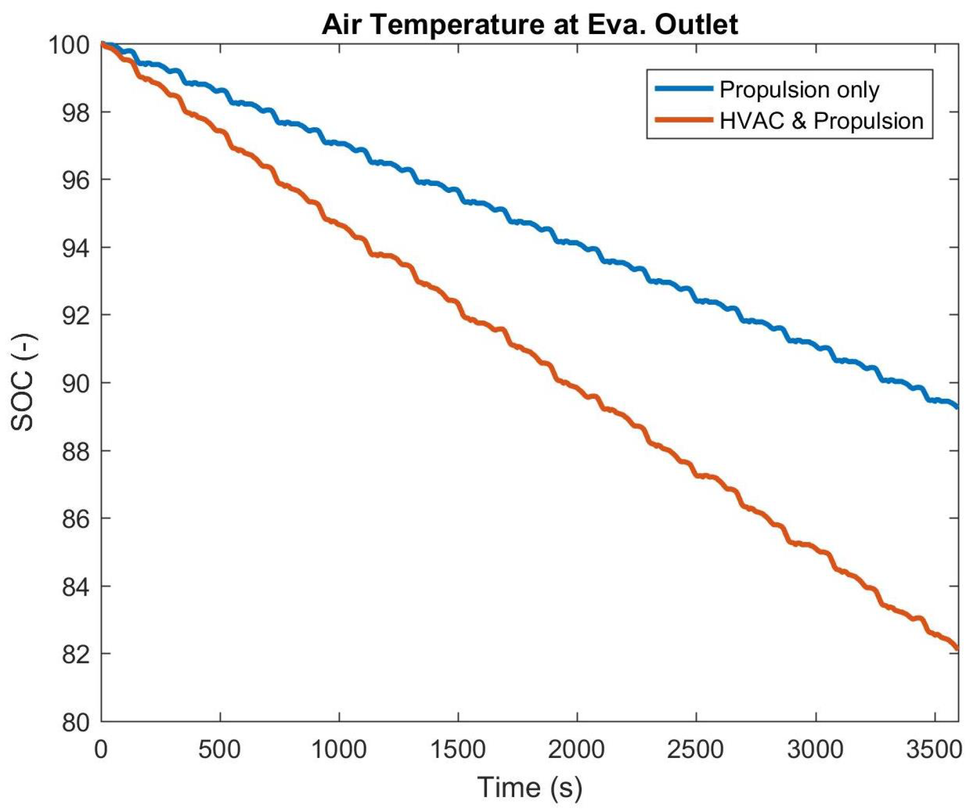
• Unsteady analysis of energy consumption: Two different HVAC working conditions were considered for the unsteady analysis of energy consumption. The first condition involves one person in the car, driving at a constant speed for 40 min on a hot summer day. The analysis compares the energy consumed by the HVAC during the drive period in two scenarios: one in which the driver enters a hot car and starts driving immediately and another where the driver enters a car that has undergone a precooling phase. The comparison shows that the energy consumption during the driving period without a precooling phase is 16% greater than with a precooling phase. However, the total energy consumed with precooling is 25% higher than without precooling, but this does not affect the energy delivered by the batteries during the drive. The second condition simulates the behavior of the HVAC system during a regulated driving cycle (ECE 15 driving cycle) that simulates urban mobility. In this case, the HVAC system increases the total energy consumption of the electric vehicle by 40%.
• Importance and future work: The contribution of the HVAC system is significant in the overall energy consumption of an electric vehicle. Therefore, a computational model that allows us to evaluate the electrical consumption of the HVAC system is crucial to improving the efficiency of electric mobility. The methodology framework proposed in this article can be extended to other HVAC systems and applied in different scenarios, allowing more robust optimization techniques for such systems. This approach shows potential practical implications, such as in a tool for describing the dynamic behavior of systems in the vehicle to compare different solutions. In an example, one can compare the energy consumption with different heat exchangers in the evaporator or condenser before building a prototype. Moreover, the dynamic simulation shown in this paper can be a basis for the optimization of a control system for the HVAC system. Hence, the methodologies presented in this paper are very useful for electric vehicle manufacturers or HVAC system developers.

References

1. Catano, J.; Zhang, T.; Wen, J.T.; Jensen, M.K.; Peles, Y. Vapor compression refrigeration cycle for electronic cooling—Part I: Dynamic modeling and experimental validation. Int. J. Heat Mass Transf. 2013, 66, 911–921. [Google Scholar] [CrossRef]
2. Nunes, T.; Vargas, J.; Ordonez, J.; Shah, D.; Martinho, L. Modeling, simulation and optimization of a vapor compression refrigeration system dynamic and steady state response. Appl. Energy 2015, 158, 540–555. [Google Scholar] [CrossRef]
3. Heimel, M.; Berger, E.; Posch, S.; Stupnik, A.; Hopfgartner, J.; Almbauer, R. Transient cycle simulation of domestic appliances and experimental validation. Int. J. Refrig. 2016, 69, 28–41. [Google Scholar]
4. Yin, X.; Wang, X.; Li, S.; Cai, W. Energy-efficiency-oriented cascade control for vapor compression refrigeration cycle systems. Energy 2016, 116, 1006–1019. [Google Scholar] [CrossRef]
5. Wang, W.; Ren, J.; Yin, X.; Qiao, Y.; Cao, F. Energy-efficient operation of the thermal management system in electric vehicles via integrated model predictive control. J. Power Sources 2024, 603, 234415–234427. [Google Scholar]
6. Liang, K.; Wang, M.; Gao, C.; Dong, B.; Feng, C.; Zhou, X.; Liu, J. Advances and challenges of integrated thermal management technologies for pure electric vehicles. Sustain. Energy Technol. Assessments 2021, 46, 101319. [Google Scholar] [CrossRef]
7. Ibrahim, A.; Jiang, F. The electric vehicle energy management: An overview of the energy system and related modeling and simulation. Renew. Sustain. Energy Rev. 2021, 144, 111049. [Google Scholar] [CrossRef]
8. Zhao, L.; Zhou, Q.; Wang, Z. A systematic review on modelling the thermal environment of vehicle cabins. Appl. Therm. Eng. 2024, 257, 124142. [Google Scholar] [CrossRef]
9. He, L.; Jing, H.; Zhang, Y.; Li, P.; Gu, Z. Review of thermal management system for battery electric vehicle. J. Energy Storage 2023, 59, 106443. [Google Scholar] [CrossRef]
10. Karimshoushtari, M.; Kordestani, M.; Shojaei, S.; Dönmez, B.; Rashid, M.; Weslati, F.; Bouyoucef, K. On the applicability of advanced model-based strategies to control of electrified vehicle thermal systems. Energy 2023, 283, 128791. [Google Scholar] [CrossRef]
11. Narimani, M.; Emami, S.; Banazadeh, A.; Modarresi, A. A unified thermal management framework for electric vehicles: Design and test bench implementation. Appl. Therm. Eng. 2024, 248, 123057. [Google Scholar] [CrossRef]
12. Lahn, F.; Chen, J.; Li, W. Effect of urban microclimates on dynamic thermal characteristics of a vehicle cabin. Case Stud. Therm. Eng. 2023, 49, 103162. [Google Scholar] [CrossRef]
13. Barlow, T.; Latham, S.; McCrae, I.; Boulter, P. A Reference Book of Driving Cycles For Use in The Measurement of Road Vehicle Emissions; TRL Published Project Report; Crowthorne House: Berkshire, UK, 2009. [Google Scholar]
14. Fayazbakhsh, M.A.; Bahrami, M. Comprehensive Modeling of Vehicle Air Conditioning Loads Using Heat Balance Method; SAE Technical Paper 2013-01-1507; SAE: Warrendale, PA, USA, 2013. [Google Scholar] [CrossRef]
15. Özışık, M. Heat Transfer: A Basic Approach; McGraw-Hill: New York, NY, USA, 1985. [Google Scholar]
16. Wagner, W.; PrussVaghela, A. The IAPWS Formulation 1995 for the Thermodynamic Properties of Ordinary Water Substance for General and Scientific Use. J. Phys. Chem. Ref. Data 2002, 31, 387–535. [Google Scholar] [CrossRef]
17. Zhao, Y.; Liang, Y.; Sun, Y.; Chen, J. Development of a mini-channel evaporator model using {R1234yf} as working fluid. Int. J. Refrig. 2012, 35, 2166–2178. [Google Scholar] [CrossRef]
18. Mendoza-Miranda, J.; Ramírez-Minguela, J.; Muñoz-Carpio, V.; Navarro-Esbrí, J. Development and validation of a micro-fin tubes evaporator model using {R134a} and {R1234yf} as working fluids. Int. J. Refrig. 2015, 50, 32–43. [Google Scholar] [CrossRef]
19. Kandlikar, S.G.; Steinke, M.E. Predicting heat transfer during flow boiling in minichannels and microchannels. Trans. Am. Soc. Heat. Refrig. Air Cond. Eng. 2003, 109, 667–676. [Google Scholar]
20. Kandlikar, S.G. A general correlation for saturated two-phase flow boiling heat transfer inside horizontal and vertical tubes. J. Heat Transf. 1990, 112, 219–228. [Google Scholar] [CrossRef]
21. Petukhov, B.; Popov, V. Theoretical calculation of heat exchange and frictional resistance in turbulent flow in tubes of an incompressible fluid with variable physical properties (Heat exchange and frictional resistance in turbulent flow of liquids with variable physical properties through tubes). High Temp. 1963, 1, 69–83. [Google Scholar]
22. Gnielinski, V. New equations for heat and mass-transfer in turbulent pipe and channel flow. Int. Chem. Eng. 1976, 16, 359–368. [Google Scholar]
23. Kakaç, S.; Shah, R.; Aung, W. Handbook of Single-Phase Convective Heat Transfer, (Chapter 3) Laminar Convective Heat Transfer in Ducts; A Wiley Interscience Publication, Wiley: Hoboken, NJ, USA, 1987. [Google Scholar]
24. Chang, Y.J.; Wang, C.C. A generalized heat transfer correlation for Iouver fin geometry. Int. J. Heat Mass Transf. 1997, 40, 533–544. [Google Scholar] [CrossRef]
25. Cavallini, A.; Del Col, D.; Doretti, L.; Matkovic, M.; Rossetto, L.; Zilio, C.; Censi, G. Condensation in Horizontal Smooth Tubes: A New Heat Transfer Model for Heat Exchanger Design. Heat Transf. Eng. 2006, 27, 31–38. [Google Scholar] [CrossRef]
26. ASHRAE Handbook. Fundamentals; American Society of Heating, Refrigerating and Air-conditioning Engineers: Peachtree Corners, GA, USA, 1997. [Google Scholar]
27. Bolz, R. CRC Handbook of Tables for Applied Engineering Science; CRC Handbook Series; Taylor & Francis: Boca Raton, FL, USA, 1973. [Google Scholar]
28. Fletcher, B.; Saunders, C. Air change rates in stationary and moving motor vehicles. J. Hazard. Mater. 1994, 38, 243–256. [Google Scholar] [CrossRef]
29. ISO 8996:2004; Ergonomics of the Thermal Environment—Determination of Metabolic Rate. International Organization for Standardization: Geneva, Switzerland, 2004.
Figure 1. Thermal loads acting on the vehicle cabin.
Applsci 15 03514 g001
Figure 2. Scheme of connections between the four devices in the HVAC system and the heat transfer processes in the evaporator and condenser.
Applsci 15 03514 g002
Figure 3. Schematic view of the real commercial air conditioning system: (A) compressor, (B) condenser, (C) fans, (D) receiver dryer, (E) TXV, (F) blower, (G) evaporator, (H) bypass valve.
Applsci 15 03514 g003
Figure 4. Temperature trend inside the climatic chamber for case 1 (left) and for case 2 (right).
Applsci 15 03514 g004
Figure 5. Temperature of air exiting the evaporator. Comparison between the simulation results (lines) and experimental ones (dots) (case 1 (left) and case 2 (right)).
Applsci 15 03514 g005
Figure 6. Evaporating and condensing pressure obtained for case 1 (left) and for case 2 (right).
Applsci 15 03514 g006
Figure 7. Thermal loads and cabin temperature obtained in the case with precooling. A dashed line is drawn in correspondence with 1200 s.
Applsci 15 03514 g007
Figure 8. Thermal loads and cabin temperature obtained in the case without precooling.
Applsci 15 03514 g008
Figure 9. Vehicle velocity during the regulated driving case.
Applsci 15 03514 g009
Figure 10. Air flow rate which enters inside the vehicle due to the infiltration.
Applsci 15 03514 g010
Figure 11. Relative contribution of the thermal loads.
Applsci 15 03514 g011
Figure 12. Thermal loads and cabin temperature obtained for the ECE 15 case.
Applsci 15 03514 g012
Figure 13. State of charge of the batteries with (red line) and without (blue line) the employment of the HVAC system.
Applsci 15 03514 g013