Abstract
Global geomagnetic field models typically have low spatial resolution, whereas regional models are constrained by boundary effects and limited truncation levels. To address these limitations, this study introduces a novel regional geomagnetic anomaly field model called the regional associated Legendre polynomials magnetic model (R−ALPOLM). This model employs the associated Legendre polynomials method, which combines the QR decomposition approach and a comprehensive evaluation index formula to enhance the computational efficiency of parameter estimation. In addition, it allows for scientific and intuitive determination of the optimal truncation level of the model. The overall prediction accuracy of the model is significantly enhanced by identifying and re-predicting outliers using the exponential moving average approach. The results indicate that the degree 83 R−ALPOLM achieves a root mean square error (RMSE) of 3.21 nT. Compared to traditional models, the proposed model exhibits lower error rates, highlighting its superior efficiency and predictive accuracy. This underscores the potential value of the proposed model in both scientific research and practical applications.
1. Introduction
The geomagnetic field—an intrinsic vector field of the Earth—is generated through the interplay of the liquid outer core, magnetic materials in the mantle and crust, and the combined effects of internal and external current systems [1,2]. The presence of a geomagnetic field can be confirmed through geomagnetic measurements and observations of auroral phenomena in high-latitude regions. Furthermore, the geomagnetic field plays a crucial role in supporting biological activity in the Earth’s ecosystem and acts as a natural barrier to protect the Earth’s surface from direct exposure to energetic particle radiation [3]. Geomagnetic fields have significant application potential in areas such as target detection, motion carrier navigation, and missile guidance [4,5,6,7]. A critical challenge in these applications lies in generating high-precision reference maps, which require extensive high-resolution geomagnetic measurements and the support of efficient and accurate modeling technologies.
Geomagnetic field modeling techniques can be broadly categorized into global and regional modeling. Global modeling provides magnetic field distributions on a worldwide scale, making it suitable for large-scale geomagnetic studies; however, when the focus shifts to the magnetic field structure of localized regions, when only regional geomagnetic data are available, or when higher-resolution magnetic field characterization is required, the significance of regional modeling becomes particularly pronounced. Regional geomagnetic field modeling is typically performed using numerical fitting techniques and mathematical–physical modeling approaches. These latter approaches are based on mathematical–physical theories, including rectangular harmonic analysis (RHA) [8,9], spherical cap harmonic analysis (SCHA) [10,11], revised spherical cap harmonic analysis (R-SCHA) [12], and inversion of equivalent sources [13]. These approaches are often constrained by truncation levels, extension effects, and boundary effects. In contrast, numerical fitting approaches do not depend on potential theory. Instead, they utilize a set of functions or polynomials to model the detailed structure of a geomagnetic field in a localized region. Although Taylor polynomials use basis functions in exponential form to characterize physical quantities, they are not suitable for constructing higher-degree models due to their non-orthogonality, which significantly increases computational complexity during inversion. Legendre polynomials, with orthogonal properties, help to simplify modeling processes and enhance the truncation level of the model, allowing for a more accurate representation of the magnetic field at smaller scales. For instance, the 50th-degree small-scale regional Legendre polynomial model developed by Au et al. can capture magnetic anomaly information within a scale range of approximately 0.4 km, with the average error in fitting experimental data maintained within 30 nT. [14].
The Legendre polynomial method for regional geomagnetic field modeling has several limitations. First, the existing Legendre polynomials are usually simplified versions of the associated Legendre functions [15], which limits the accuracy of the model. Second, boundary effects are typically addressed by refining the boundary data, which enhances the accuracy of local data but also increases the computational complexity and workload. In addition, there may be inconsistencies in the data collected at different time points, affecting the overall accuracy of the model. Furthermore, the truncation level of the model remains insufficient, resulting in significant fitting errors that restrict its applicability to magnetic fields with small-scale distributions.
In this study, global geomagnetic anomaly field grid data derived from the Earth Magnetic Anomaly Grid (EMAG) model are used to create a basic model of localized regional geomagnetic anomalies—referred to as the R−ALPOLM—by employing associated Legendre polynomials. The model enhances the computational efficiency of parameter estimation through incorporation of the QR decomposition technique [16]. In addition, this study develops a comprehensive evaluation index that combines the effects of outliers with the accuracy of model predictions to determine the optimal truncation level of the model. To address the issue of boundary effects in the model, the box plot approach is first used to detect and remove outliers. Subsequently, the exponential moving average method is applied to re-predict these outliers, resulting in a high-precision regional geomagnetic anomaly field model. The combined application of these methods offers an accurate and efficient framework for regional geomagnetic anomaly modeling.
2. Principles and Methods
2.1. Associated Legendre Polynomials
Associated Legendre equations are a type of ordinary differential equation frequently encountered in physics and various technical fields, particularly emphasizing orthogonality, computational accuracy, and speed in geophysics. The standard Legendre polynomials are a special case derived from solving an associated Legendre equation. When solving the associated Legendre equation, the solutions can be categorized into two main forms: one is the direct solution form, which involves explicit mathematical expressions to directly compute the solutions; the other is the recursive form, which is obtained through recurrence relations. Although these two forms are theoretically equivalent as solutions to the equation, they differ significantly in computational efficiency and numerical stability due to their structural differences. The direct solution form has precise mathematical expressions and can directly compute associated Legendre polynomials of any degree. However, for higher-degree polynomials, the computational cost of the direct solution increases dramatically and numerical instability may occur when the truncation level is large. This is because the calculation of higher-degree polynomials involves complex mathematical operations, which are susceptible to limitations in floating-point precision, leading to the accumulation of computational errors. In contrast, the recursive form—while less elegant in theoretical analysis—is highly suitable for efficient and stable numerical computations. Recurrence relations avoid the numerical instability issues that may arise in direct solutions, particularly excelling in the computation of higher-degree polynomials. In this study, the final recurrence formula for the associated Legendre polynomials we used is as follows [17]:
The x in Equation (1) represents the longitude or latitude value, k denotes the degree of the associated Legendre polynomials, and m represents the ordinal number of the summed terms.
2.2. Basic Modeling Methods
Modeling the geomagnetic field using the associated Legendre polynomials involves creating a basis function system, solving the coefficient matrix, and using the basis function series to predict observations. Assuming that the geomagnetic element of the geomagnetic field is B, the basis function system is jointly constructed using the associated Legendre polynomials , where and denote the normalized latitude and longitude, respectively; N denotes the maximum degree of the expansion; n indicates the order of the associated Legendre polynomial expansion; and A is the matrix of model coefficients. The associated Legendre polynomials exhibit orthogonality, which satisfies Equation (2):
Based on this, the basic model equations of the geomagnetic field in the localized region can be constructed using Equation (3):
which can be simplified as , where the matrix D is constructed from associated Legendre polynomials, as shown in Equation (4), and B represents the observed data sequence. The coefficient matrix A is typically solved using the least squares method. However, as the truncation level of the expansion increases, its numerical instability is significantly exacerbated, often leading to failure to obtain a solution [18,19]. Although the Cholesky decomposition method offers higher computational efficiency, it is only applicable to symmetric positive definite matrices and also faces numerical stability-related challenges at high orders [20]. The singular value decomposition (SVD) method, while effective in handling ill-conditioned matrices, presents a significant increase in computational complexity as the order rises [21]. In contrast, the QR decomposition method demonstrates outstanding numerical stability, effectively addressing ill-conditioned matrix problems in high-order polynomial fitting while maintaining moderate computational complexity and balancing precision with efficiency. Therefore, based on the comprehensive consideration of numerical stability, computational efficiency, and applicability, this study employs the QR decomposition method as the optimal approach for solving the coefficient matrix. The fundamental principle of QR decomposition lies in its orthogonalization process, which transforms the column vectors of a matrix into an orthogonal basis while generating an upper triangular matrix. This process ensures high stability and efficiency in numerical computations. In this study, QR decomposition is applied to solve the coefficient matrix of the geomagnetic field model, where its orthogonality guarantees computational accuracy, and the upper triangular structure significantly simplifies subsequent solution procedures. If the final matrix formed by the associated Legendre polynomials is D, the QR decomposition method effectively preserves the stability of the numerical computation and reduces the computational complexity by transforming matrix D into an orthogonal matrix Q and an upper triangular matrix R. In Equation (6), represents the pseudo-inverse of R. For the upper triangular matrix R, the pseudo-inverse is its inverse.
The model calculations yield a coefficient matrix A, which can subsequently be used to make predictions of the modeled data in the region.
3. Data and Modeling Results
3.1. Data Sources and Pre-Processing
Geomagnetic anomalies are residual magnetic fields derived by removing the main, varying, and induced magnetic fields from the global magnetic field, also known as the crustal or lithospheric magnetic field. EMAG is compiled based on satellite magnetometry, ocean magnetometry, and aeromagnetic measurements, and the latest EMAG2v3 database was released by the U.S. National Centers for Environmental Information (NCEI) in 2016 [22] and updated in 2017. This database includes converted 4 km altitude and sea level data, formatted as a grid with abundant available data points as well as high fidelity and accuracy, with the minimum resolution reaching 2’ (approximately 3.7 km) globally. These data can be applied for aeromagnetic surveys, ocean exploration, geomagnetic navigation, and other related applied research [23,24] (EMAG2v3 data were obtained from https://www.ncei.noaa.gov/products/earth-magnetic-model-anomaly-grid-2 (accessed on 15 December 2024)).
To maintain the orthogonality of the associated Legendre polynomials, it is crucial to normalize the latitude and longitude coordinates of the data, ensuring that the values lie within the interval [−1, 1]:
where represent the value of the latitude and longitude coordinates of a data point, , denote the maximum and minimum values of the latitude coordinates, denote the maximum and minimum values of the latitude and longitude coordinates, and represent the results of normalizing the latitude and longitude coordinates, respectively.
3.2. Regional Geomagnetic Anomaly Field Model Construction
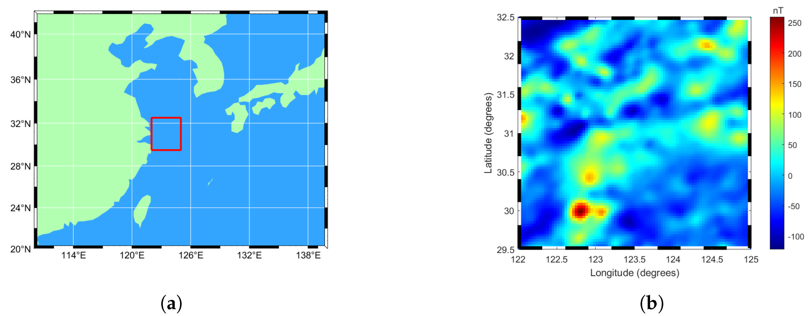
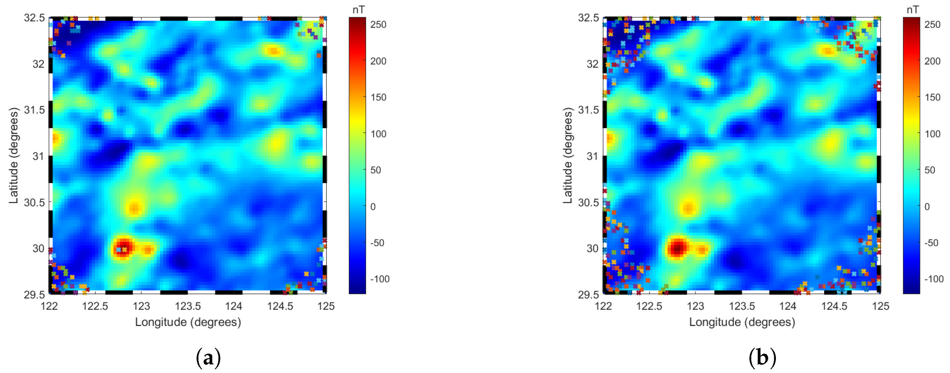
In this study, the Northwest Pacific Ocean—specifically, the 3° × 3° area from 122° E to 125° E in longitude and 29.5° N to 32.5° N in latitude (the area marked by the red box in Figure 1a)—was selected as the study area. This area, which covers approximately 160,000 square kilometers and contains 8100 data points, was assessed based on the sea-level dataset. As illustrated in Figure 1b, the spatial distribution of the geomagnetic anomalies in the study area is clearly characterized, and the statistics provided in Table 1 highlight the significant variations regarding the geomagnetic anomalies in the area. Furthermore, there are several areas with high geomagnetic anomaly values in the region, which provides good conditions for verifying and comparing the accuracy and applicability of various modeling approaches. To construct and validate the model, of the data (i.e., 6480 data points) were randomly selected from the 8100 points in the selected region as the training dataset for the model; meanwhile, the remaining (i.e., 1620 data points) were used as the test dataset for the model. This data partitioning approach ensures an unbiased evaluation of the model’s performance on independent data. To objectively assess the model’s predictive accuracy, the root mean square error (RMSE) was selected as the key index, which is calculated as follows:
where n represents the number of samples, denotes the predicted value of the model for the ith data point, and represents the true value for the ith data point. The smaller the RMSE value, the smaller the difference between the predicted result and the true value of the model, which indicates that the predictive performance of the model is superior. Through calculating the RMSE, we can quantitatively assess the prediction accuracy of the model and provide a scientific basis for the optimization and selection of the model.
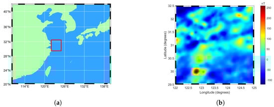
Figure 1.
Overview of the experimental area: (a) Scope of the experimental area. (b) Distribution of geomagnetic anomalies in the experimental area. The data have a horizontal resolution of 2 arcminutes.

Table 1.
Basic experimental data.
Previous studies [14] have highlighted that the truncation level and the resolution of boundary effects are critical factors in constructing regional geomagnetic anomaly models. In regional geomagnetic field modeling, the truncation level refers to the maximum degree of the modeling model expansion used, which determines the resolution and complexity of the model. The selection of the optimal truncation level is crucial, as it balances the trade-off between model accuracy and computational efficiency. A higher truncation level captures finer details of the field but increases the computational complexity, while a lower truncation level simplifies calculations but may omit significant features. Therefore, the optimal truncation level is determined through comprehensive consideration of the error analysis results and computational efficiency. Regarding boundary effects, the prediction of data within the modeling region is essentially an interpolation problem, where points exhibit continuous relationships with surrounding points. However, at the boundaries, the boundary points have vacant data outside the region, which can result in significant deviations in the model predictions at the boundary points. Figure 2a illustrates the relationship between the truncation level and the number of outliers. The RMSE was calculated using the training data and the number of outliers, which was determined using the test data through the box plot method (as will be detailed later in this section). As shown in Figure 2b, when the truncation level is less than 10, the model is in an underfitting state, leading to a certain number of outliers. As the truncation level increased gradually from 10, the accuracy of the model training improved, with the RMSE reaching its minimum value of 0.41 nT at the 85th degree. This accuracy was maintained up to approximately the 104th degree, after which the RMSE started to increase gradually and slightly. The relationship between the number of outliers and the truncation level follows an approximately exponential trend, expressed as . As the truncation level increases from 0 to 87, the number of outliers increases from 0 to 100. With a further increase in the truncation level from 88 to 97, the number of outliers increases from 100 to 200. Subsequently, as the truncation level increases from 98 to 300, the number of outliers continues to increase, before decreasing slightly to 100 from 200 when the truncation level spans from 88 to 97. As the truncation level increased from 98 to 105, the detected outliers also increased. At a truncation level of 85, 93 outliers were identified, which comprised of the total number of data points. When the truncation level increased to 104, the number of detected outliers increased to 270, approximately three times the original number. Figure 3 illustrates the distribution of outliers at truncation levels of 85 and 104. The outliers were primarily concentrated at the four corners of the region’s boundary. At the 104th truncation level, the number of outliers increased significantly and extended further into the interior of the region.
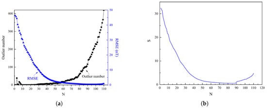
Figure 2.
Determination of the optimal truncation level for the R−ALPOLM: (a) Relationship between the number of outliers and RMSE with truncation level. (b) Determination of the optimal truncation level for the R−ALPOLM.
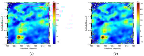
Figure 3.
Distribution of outliers in the R−ALPOLM at different degrees, with ‘x’ symbols representing outliers: (a) Distribution of 85th degree model outliers. (b) Distribution of 104th degree model outliers.
To more accurately and rationally determine the optimal truncation level, this study proposes a comprehensive evaluation index formula that combines the RMSE and the number of outliers A, and fully considers their impact on the overall assessment. The formula is as follows:
In Equation (9), and represent the weight parameters and satisfy ; meanwhile, denotes a nonlinear function of the number of outliers A, which is used to adjust the impact of outliers on the comprehensive evaluation index. Specifically, as the number of outliers increases, the negative impact on the comprehensive evaluation index also increases. The explicit form of is given by:
In Equation (10), represents a threshold value and k represents a constant greater than 1, which is used to amplify the impact of outliers that exceed the threshold.
During the model training phase, the RMSE was selected as the primary evaluation index. The value of the weight was set to 0.7 and the value of was set to 0.3. is taken as the threshold value of of the number of checkpoints (i.e., it is 113). This threshold value was based on a statistical analysis of the dataset and the requirements for identifying outliers. Furthermore, k was set to 1.2 to enhance the sensitivity of the model to outliers. As shown in Figure 2b, analyzing the trend of the comprehensive evaluation index in relation to the truncation level revealed that the index remained highly stable between the 81st and 89th truncation levels, consistently falling within the range of 0.56 to 0.59. The integrated evaluation index value reached a minimum of 0.5622 at the 83rd degree. This result indicates that the 83rd degree is the optimal truncation level for the model, achieving a good balance between model complexity and prediction performance. Thus, the 83rd degree was selected as the optimal truncation level of the R−ALPOLM in this study, and post-processing of the predicted outliers was performed on this basis to enhance the performance of the model.
Traditional approaches to handling boundary effects typically involve adding boundary data points to control errors, thereby enhancing the fitting degree of the model and overcoming boundary issues. However, when constructing a model, measured data are considered the most reliable. Artificial interpolation—which involves generating synthetic data based on measured values for use as training data—can introduce unnecessary errors. These errors vary depending on the distribution density of the measured data, leading to a certain level of error during the initial stages of model construction.
The data presented in Table 2 indicate the overall RMSE after removing the prediction outliers. The results indicate that the overall prediction accuracy of the model remained high after excluding the predicted outliers, and the RMSE decreased with increasing truncation level. Furthermore, through the selection of an appropriate truncation level, the number of prediction outliers can be limited to a smaller proportion of the total number of checkpoints. Consequently, including significant predicted outliers in the evaluation of model accuracy to determine the truncation level is not ideal, as it does not accurately reflect the prediction performance of higher-degree models.
Table 2.
Effect of outliers on model accuracy at different truncation levels.
In light of this, this study does not focus on the original observations when addressing boundary effects but, instead, employs a strategy of post-processing the abnormal predicted values at the boundaries based on the model to enhance the overall prediction performance. This approach aims to reduce the negative impacts of boundary effects on model performance through optimizing the prediction mechanism within the model to achieve more accurate prediction results.
Outlier detection was performed using the box plot method, which visualizes the distribution of raw geomagnetic data by dividing the dataset into four equal parts based on three quartiles: the lower quartile (Q1), the median (Q2), and the upper quartile (Q3). Specifically, Q1 separates the lowest of the data, Q2 (the median) divides the data into two equal halves, and Q3 marks the boundary below which of the data falls. This division effectively partitions the dataset into four distinct segments, each representing of the data, ordered from the smallest to largest values. The difference between the upper and lower quartiles is known as the Interquartile Range (IQR). Values greater than the upper quartile by 1.5 times the IQR or smaller than the lower quartile by 1.5 times the IQR are typically classified as outliers when detecting predicted outliers using the box-and-line plot method. This method is highly robust as the IQR is less affected by outliers.
The moving average is a widely used statistical technique in data analysis and time series forecasting. Its primary purpose is to minimize randomness by smoothing data to better extract trend features. For regional geomagnetic data, which typically exhibit continuity, outlier prediction can be performed by applying the moving average method to smooth the predicted data values of surrounding points (N points of radius d). This approach enables the re-prediction of outliers. To address predicted outliers in a dataset , the following steps can be taken:
Step 1: Compute the upper quartile and the lower quartile .
Step 2: Determine the interquartile range .
Step 3: Detect predicted outliers: if , then is not an outlier; otherwise, is an outlier.
Step 4: Use the model coefficient matrix A to predict the geomagnetic data for the surrounding point coordinates, in order to obtain the surrounding point data values .
Step 5: Calculate the surrounding point average for each outlier: .
The obtained result is the result of the re-prediction of the predicted outliers.
3.3. Model Accuracy Evaluation Analysis
To evaluate the superiority of the R−ALPOLM in regional geomagnetic field modeling, comparative experiments were conducted against the Taylor polynomial model (TPM) and the Legendre polynomial model (LPM). These models are based on Taylor polynomials and traditional Legendre polynomials, respectively. The Taylor polynomial is a widely used mathematical tool that provides local approximations of functions around a specific point. In the context of geomagnetic field modeling, it can also be employed to approximate variations in geomagnetic elements. For a given geomagnetic element B, the center point of the modeled region is selected as the expansion point of the Taylor polynomial. The normalized latitude and longitude coordinates of the center point are denoted by and , A denotes the matrix of model coefficients, and the modeling formula is expressed as in Equation (11) [25,26]:
The direct solution formula for the traditional Legendre polynomials is shown in Equation (12):
In Equation (12), represents the integer part of , where n is the degree of the Legendre polynomial, and m denotes the order of the summation terms. The fundamental model equations used for both Legendre polynomials and associated Legendre polynomials are identical, with the key difference lying in the polynomial . By substituting Equation (12) into Equation (3), the subsequent methods and steps for solving the coefficient matrix remain the same.
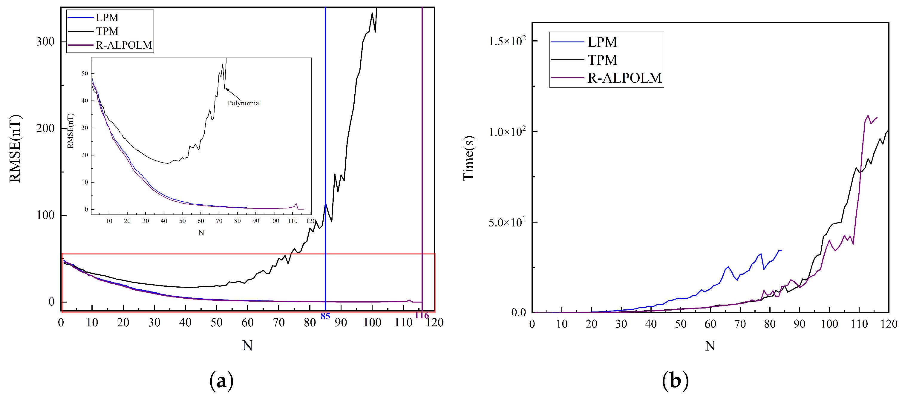
The experimental data originated from the training dataset described in Section 3.2, and the results illustrated in Figure 4 were obtained by comparing the training accuracy and runtime of the three models at different truncation levels. As illustrated in Figure 4a, the RMSE of the LPM and the R−ALPOLM proposed in this study decreased rapidly as the truncation level increased, where the RMSE value of the R−ALPOLM was slightly lower than that of the LPM. However, the LPM encounters a singular value problem at the 85th degree; thus, it is incapable of further execution. Conversely, the proposed model demonstrated stable performance, operating successfully up to the 116th degree before encountering the singular value issue. The RMSE value of the TPM was substantially higher than those for the other two models, showing a sharp increase after descending to the 42th degree and exhibiting greater fluctuations after the 42th degree.
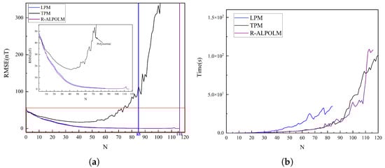
Figure 4.
RMSE and running time of the three models at different degrees: (a) RMSE. (b) Running time.
Figure 4b illustrates the runtime performance of the three models. The runtime of all models increased as the truncation level increased. The overall runtimes of the TPM and R−ALPOLM were comparable, whereas the LPM exhibited a significantly higher runtime than the other two models. Notably, the singular value problem occurred at the 43rd degree for the TPM, which explains the sharp increase in the RMSE value after the 42nd degree. The appearance of the singular value solution in the TPM runtime indicates that it does not have significant reference value. Considering its higher-degree fitting ability and runtime efficiency, the proposed R−ALPOLM exhibited a clear advantage.
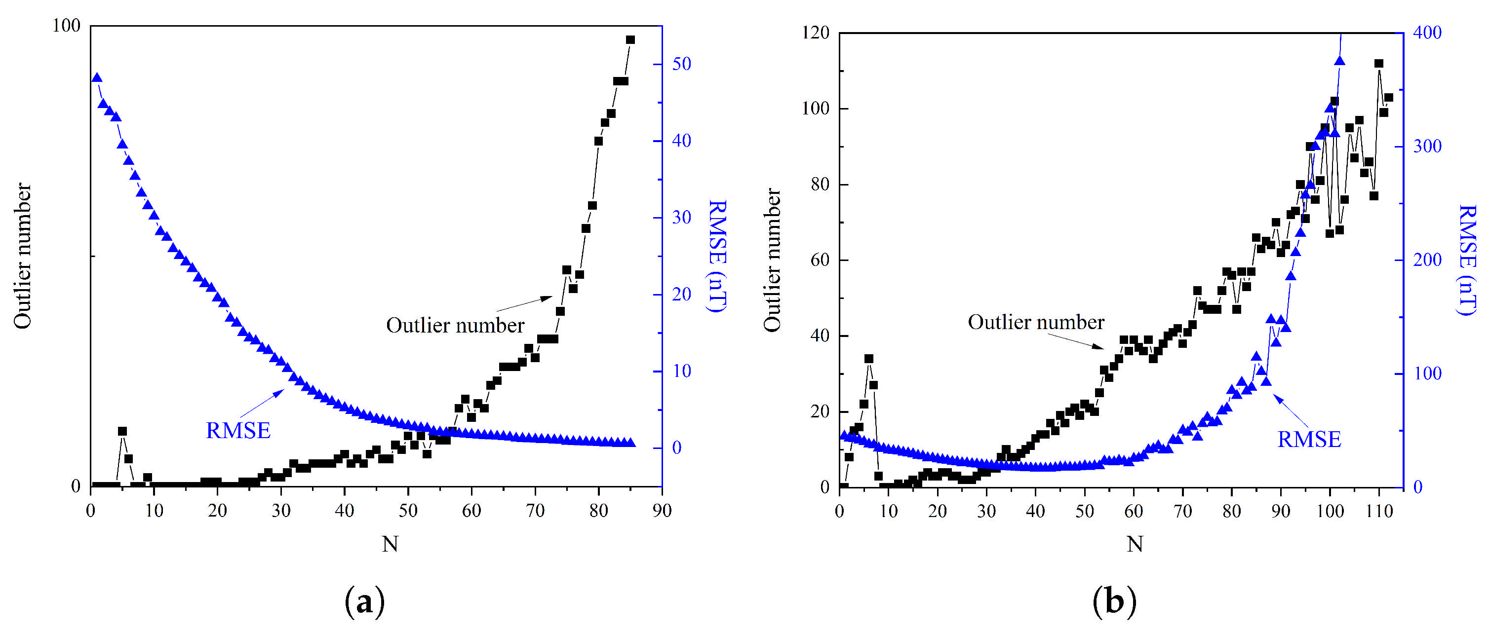
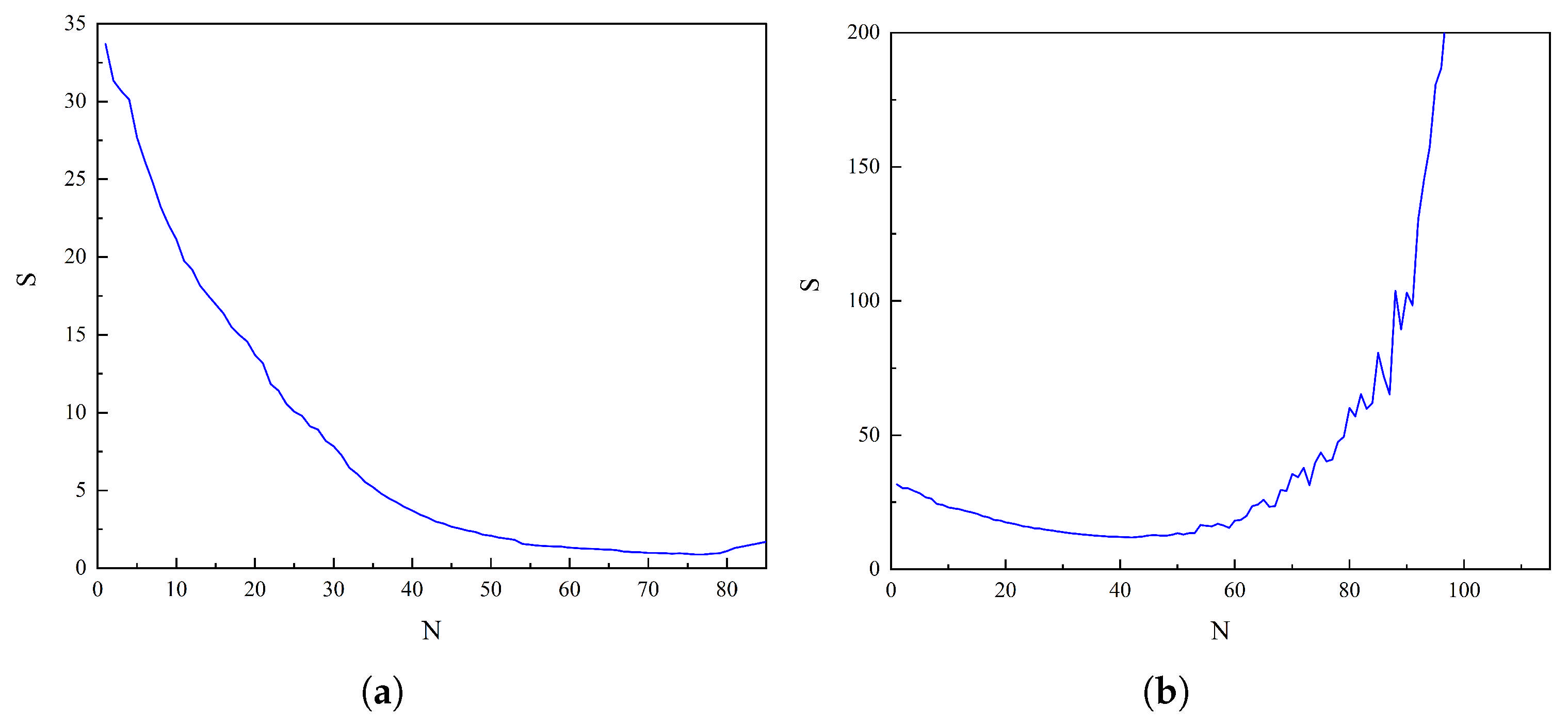
Figure 5 shows the variations in RMSE and the number of outliers for TPM and LPM at different degrees. As illustrated in Figure 5a, the LPM and R−ALPOLM exhibited similar results when the truncation level increased, with their RMSE values decreasing while the number of outliers gradually increased. At a truncation level of 85, the RMSE reached a minimum of 0.59 nT, whereas the number of outliers increased to a maximum of 97. To evaluate the combined impact of the RMSE and number of outliers on the overall model performance, the comprehensive evaluation index (defined in Equation (9)) was applied. The obtained results are illustrated in Figure 6a. As shown in Figure 6a, the comprehensive evaluation index steadily decreased as the truncation level increased, reaching a minimum value of 0.8749 at the 76th degree. Beyond this point, the index began to increase gradually, Based on this analysis, the optimal truncation level for the LPM was identified as the 76th degree, corresponding to the outlier number of 43 points and representing approximately of the total number of points. As shown in Figure 5b, the trend in RMSE of the TPM across truncation levels can be categorized into three phases: a slow decrease in the initial phase, followed by local stabilization and, finally, a sharp increase. For truncation levels lower than 42, the RMSE gradually decreased, reaching a minimum value of 16.9 nT at degree 42. Between degrees 42 and 51, the RMSE remained relatively stable, fluctuating within a range of approximately 1 nT. However, from degree 52 onward, the RMSE increased dramatically, exceeding 400 nT at degree 103. Simultaneously, the change in the number of outliers exhibited a specific pattern. The number of outliers exhibited continuous fluctuations within the first 7 degrees. The number of outliers then increased rapidly from the 8th to the 90th degree. After the 90th degree, although the number of outliers continued to increase in general, significant fluctuations occurred. Considering the influences of the RMSE and the number of outliers on the overall model, the results obtained when applying the comprehensive evaluation index formula (Equation (9)) are shown in Figure 6b. As illustrated in Figure 6b, the comprehensive evaluation index decreased steadily as the truncation level increased, reaching a minimum value of 11.9086 at the 42nd degree. After this point, the index increased rapidly, reaching a value of 4507.089 at the 112th degree. Thus, the optimal truncation level of the TPM was determined to be the 42nd degree.
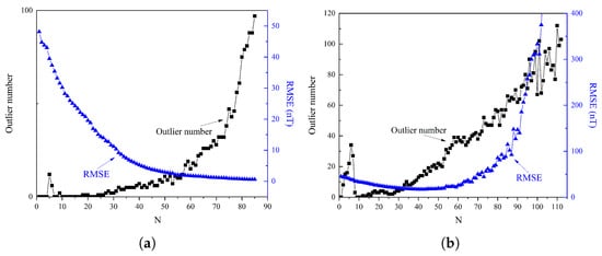
Figure 5.
Relationship between the number of outliers and RMSE with truncation level for: (a) The LPM. (b) The TPM.
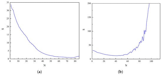
Figure 6.
Optimal truncation level for the (a) LPM and (b) TPM.
Next, we compared the performance of the R−ALPOLM, LPM, and TPM at their respective optimal truncation levels. Table 3 presents the statistics of the predicted data for the three models. The results indicate that the maximum error value of the predicted data for the R−ALPOLM of 83rd degree was 32.60 nT, the minimum error was nT, the average error was 1.16 nT, and the RMSE was 3.21 nT, which were the lowest among the three models for all parameters. The R−ALPOLM exhibited the lowest RMSE among the models, thereby highlighting its superior prediction accuracy. The predicted data for the 76th degree LPM showed similar values for the maximum, minimum, and the average error values, compared with the R−ALPOLM; however, the RMSE value for the LPM reached 5.00 nT, indicating comparable stability, although it was slightly inferior to that of the R−ALPOLM. In contrast, the predicted values for the 42nd degree TPM differed notably from those of the first two models, particularly with the RMSE reaching 12.76 nT. This was significantly higher than those for the first two models, highlighting a disadvantage in terms of its prediction accuracy.
Table 3.
Statistics of the three model projections.
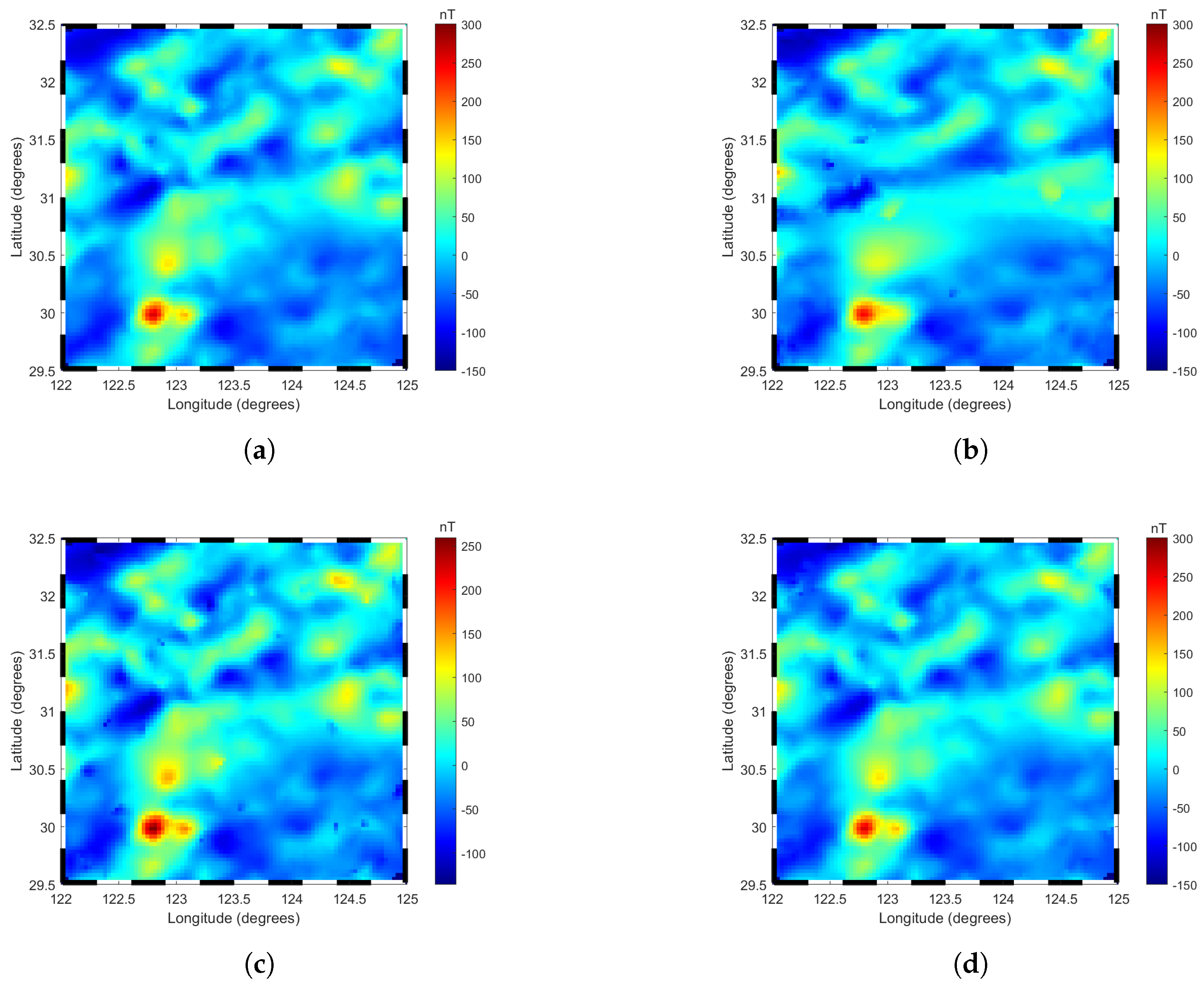
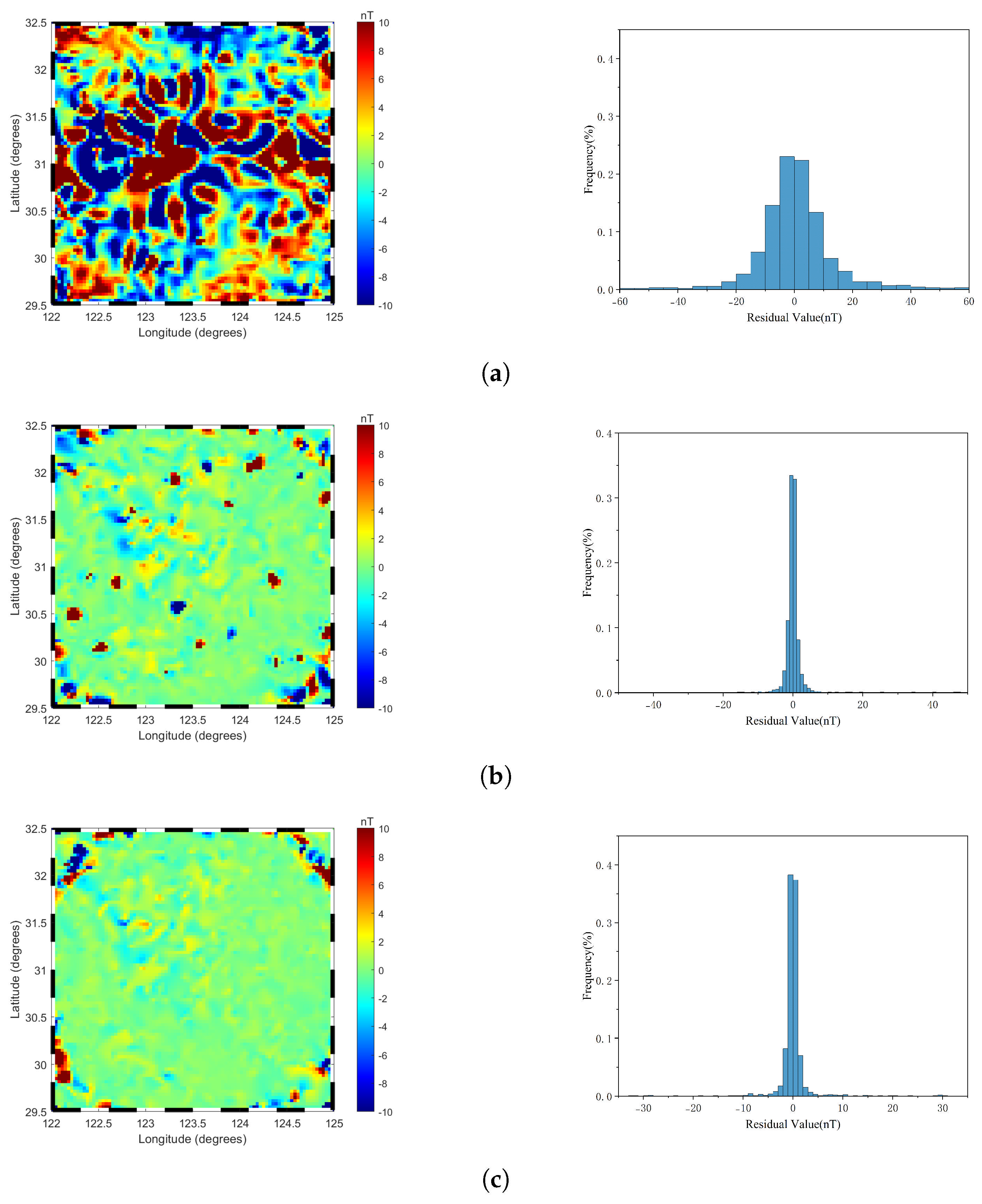
Figure 7 illustrates the two-dimensional (2D) images of local geomagnetic anomalies constructed by three models at their respective optimal truncation levels. The observations and analyses indicate that the 2D images generated by each model exhibit a high degree of consistency with the original geomagnetic anomaly data in terms of overall color distribution, effectively capturing the general characteristics of the geomagnetic anomaly field. Notably, the R−ALPOLM and LPM demonstrate significant advantages in the depiction of detailed features, as their 2D images not only align closely with the overall color distribution trends of the original data but also exhibit higher similarity in local detail characteristics. In contrast, although the TPM model maintains basic consistency with the original data in terms of overall color distribution trends, it shows obvious deficiencies in the expression of detailed features, with multiple regions displaying inconsistent color distributions compared to the original data, indicating its weaker capability in capturing local geomagnetic anomaly features. To further visually illustrate the differences in fitting accuracy among the three models, Figure 8 presents the planar residual distribution and residual histograms of the predicted results from each model. As shown in Figure 8, the R−ALPOLM model exhibits the best modeling performance, with residuals primarily concentrated within the range of ±2 nT. Moreover, the residual values in the central modeling region are generally small, indicating high fitting accuracy. Larger residuals are mainly distributed in the four corner regions of the modeling area, and their distribution pattern aligns with the anomaly point distribution characteristics described in Section 3.2. The LPM model also performs well overall, with residuals similarly concentrated within ±2 nT. However, compared to the R−ALPOLM model, its high residuals are more dispersed, appearing not only in the corner regions but also in the central modeling area, suggesting slightly inferior fitting capability for local geomagnetic anomalies compared to the R−ALPOLM model. In contrast, the TPM model exhibits significantly larger residuals, with high residuals widely distributed throughout the entire modeling region, indicating substantially lower modeling accuracy compared to the R−ALPOLM and LPM models.

Figure 7.
Two−dimensional planar data plots of the regional geomagnetic anomaly field: (a) The original data. (b) The TPM model. (c) The LPM model. (d) The R−ALPOLM model.The figure illustrates the comparison between the original data and the models constructed by TPM, LPM, and R−ALPOLM.

Figure 8.
Planar residual distribution and residual histograms of the model predictions: (a) The TPM model, (b) The LPM model, and (c) The R−ALPOLM model. The residuals are calculated as the difference between the original data and the model predictions. The figure illustrates the spatial distribution of residuals for each model, along with their corresponding histograms, providing a comprehensive comparison of the prediction accuracy.
4. Discussion and Conclusions
This study successfully developed a new regional geomagnetic anomaly field model—namely, the R−ALPOLM—using associated Legendre polynomials to enhance the accuracy and efficiency of geomagnetic field modeling. The model achieved an RMSE value of 3.21 nT, outperforming the LPM (5 nT) and TPM (12.76 nT) models considered in this study, as well as previous models (30 nT) [14], indicating its enhanced performance. This result highlights the advantage of the R−ALPOLM in accurately modeling geomagnetic anomaly fields and confirms the feasibility of enhancing the prediction accuracy through the post-processing of outliers, providing significant potential for applications in geophysical exploration, geomagnetic navigation and positioning, and other related fields.
As the degree of the model increased, the number of outliers showed a tendency to increase, primarily distributed in the boundary region of the model. These outliers typically have extremely large values, which significantly affect the overall accuracy of the model. Previous studies have addressed the boundary effect through the interpolation of additional boundary points, which can enhance the prediction accuracy of the model to some extent. As the degree of the model increases, the instability of the boundary also increases, which requires the introduction of more boundary points to compensate for this issue; however, an excessive number of boundary points can undermine the reliability of the experimental data. Furthermore, after sufficient data points are added to the boundary region, the effectiveness of mitigating the boundary effect through a high density of interpolation points begins to diminish. The results of this study indicate that properly addressing boundary outliers can significantly enhance the accuracy of the predicted data and reduce the computational complexity and workload, to some extent. There is a threshold value for the number of outliers, and appropriate weights must be applied when determining the optimal truncation level. This approach not only enhances the prediction accuracy of the model, but also effectively controls the boundary effect of the model while maintaining the credibility of the data, thereby achieving a balance between model construction and prediction accuracy. In this study, a comprehensive evaluation index formula was developed to determine the optimal truncation level, offering an alternative to commonly used methods such as the magnetic energy density, RMSE, and Chi-square information principles found in previous studies [14,27]. This new approach provides a more intuitive and scientifically grounded tool for the evaluation of model performance when selecting the truncation degree of a model.
As a limitation of this study, the model stability and outlier processing strategy require further optimization—particularly in the post-processing of outliers using the moving average approach. The selection of surrounding points plays a critical role in determining the accuracy of the re-predicted values. As such, future research can focus on enhancing model stability and refining the outlier processing strategy to achieve higher accuracy in local geomagnetic field modeling. This is expected to contribute to advancing the field of geomagnetic field modeling research.
Author Contributions
Conceptualization, L.Z. and H.L.; methodology, L.Z. and H.L.; validation, M.C. and B.Z.; formal analysis, J.O. and B.Z.; writing—review and editing, L.Z. and J.O. All authors have read and agreed to the published version of the manuscript.
Funding
This research was funded by the National Natural Science Foundation of China, grant number 42430101 and 42374050; the National Science Foundation for Outstanding Young Scholars of China, grant number 42122025.
Institutional Review Board Statement
Not applicable.
Informed Consent Statement
Not applicable.
Data Availability Statement
Geomagnetic data were obtained from https://www.ncei.noaa.gov/products/earth-magnetic-model-anomaly-grid-2 (accessed on 15 December 2024).
Acknowledgments
This research was generously funded by the National Science Foundation for Outstanding Young Scholars of China and the National Natural Science Foundation of China. We express our sincere gratitude for this support. The geomagnetic data, which were pivotal to our study, were provided by National Centers for Environmental Information and are accessible at https://www.ncei.noaa.gov/products/earth-magnetic-model-anomaly-grid-2 (last accessed on 8 January 2025). We acknowledge the crucial role these data played in our research endeavors. We appreciate the availability of this resource, which significantly contributed to our analytical approach. Our thanks are extended to the editor and the anonymous reviewers for their insightful and constructive comments, which were invaluable in enhancing the quality of this paper.
Conflicts of Interest
The authors declare no conflicts of interest.
Abbreviations
The following abbreviations are used in this manuscript:
| R−ALPOLM | Regional Associated Legendre Polynomials Magnetic Model |
| RMSE | Root Mean Square Error |
| EMAG | Earth Magnetic Anomaly Grid |
| TPM | Taylor Polynomial Model |
| LPM | Legendre Polynomial Model |
References
- Matzka, J.; Chulliat, A.; Mandea, M.; Finlay, C.C.; Qamili, E. Geomagnetic observations for main field studies: From ground to space. Space Sci. Rev. 2010, 155, 29–64. [Google Scholar] [CrossRef]
- Gubbins, D.; Herrero-Bervera, E. (Eds.) Encyclopedia of Geomagnetism and Paleomagnetism; Springer Science & Business Media: Berlin/Heidelberg, Germany, 2007. [Google Scholar]
- Erdmann, W.; Kmita, H.; Kosicki, J.Z.; Kaczmarek, Ł. How the geomagnetic field influences life on Earth–an integrated approach to geomagnetobiology. Orig. Life Evol. Biosph. 2021, 51, 231–257. [Google Scholar] [PubMed]
- Yuan, Z.F.; Liu, X.G.; Kong, D.H.; Du, C.P.; Peng, X.; Guo, H.; Xia, M.Y. Enhanced Aeromagnetic Compensation Models for Magnetic Anomaly Target Detection. IEEE Trans. Geosci. Remote Sens. 2024, 62, 1001813. [Google Scholar] [CrossRef]
- Xu, X.; Huang, L.; Liu, X.; Fang, G. DeepMAD: Deep Learning for Magnetic Anomaly Detection and Denoising. IEEE Access 2020, 8, 121257–121266. [Google Scholar]
- Tang, C.; Shi, H.; Zhang, L. Geomagnetic matching cooperative positioning method for unmanned boat cluster based on factor graph. Ocean Eng. 2024, 296, 116901. [Google Scholar] [CrossRef]
- Zhu, X.; Jia, Q.; Zhao, Y.; Song, J.; He, Y. Attitude Measurement Method of Geomagnetic/Gyro Combination based on Difference-Quotient. In Proceedings of the 2020 IEEE 4th Information Technology, Networking, Electronic and Automation Control Conference (ITNEC), Chongqing, China, 12–14 June 2020; Volume 1, pp. 841–847. [Google Scholar] [CrossRef]
- Alldredge, L. Rectangular harmonic analysis applied to the geomagnetic field. J. Geophys. Res. Solid Earth 1981, 86, 3021–3026. [Google Scholar] [CrossRef]
- Alldredge, L.R. Geomagnetic local and regional harmonic analyses. J. Geophys. Res. Solid Earth 1982, 87, 1921–1926. [Google Scholar] [CrossRef]
- Haines, G. Spherical cap harmonic analysis. J. Geophys. Res. Solid Earth 1985, 90, 2583–2591. [Google Scholar]
- Korte, M.; Holme, R. Regularization of spherical cap harmonics. Geophys. J. Int. 2003, 153, 253–262. [Google Scholar]
- Thébault, E.; Schott, J.; Mandea, M.; Hoffbeck, J. A new proposal for spherical cap harmonic modelling. Geophys. J. Int. 2004, 159, 83–103. [Google Scholar] [CrossRef]
- Harrison, C. The crustal field. Geomagnetism 1987, 1, 513–610. [Google Scholar]
- Ou, J.M.; Du, A.M.; Xu, W.Y.; Hong, M.H.; Chen, G.X.; Luo, H.; Zhao, X.D.; Bai, C.H.; Wang, Y. The Legendre polynomials modeling method of small-scale geomagnetic fields. Chin. J. Geophys. 2012, 55, 2669–2675. [Google Scholar]
- Wyld, H.W.; Powell, G. Mathematical Methods for Physics; CRC Press: Boca Raton, FL, USA, 2020. [Google Scholar]
- Björck, Å. Numerical Methods in Matrix Computations; Springer: Berlin/Heidelberg, Germany, 2015; Volume 59. [Google Scholar]
- Schweizer, W. Special Functions in Physics with MATLAB; Springer: Berlin/Heidelberg, Germany, 2021. [Google Scholar]
- Ding, F. Least squares parameter estimation and multi-innovation least squares methods for linear fitting problems from noisy data. J. Comput. Appl. Math. 2023, 426, 115107. [Google Scholar] [CrossRef]
- Golub, G.H.; Van Loan, C.F. Matrix Computations; JHU Press: Baltimore, MD, USA, 2013. [Google Scholar]
- Blaschke, S.; Stopkowicz, S. Cholesky decomposition of complex two-electron integrals over GIAOs: Efficient MP2 computations for large molecules in strong magnetic fields. J. Chem. Phys. 2022, 156, 044115. [Google Scholar] [CrossRef]
- Weiss, S.; Proudler, I.K.; Barbarino, G.; Pestana, J.; Mcwhirter, J.G. On Properties and Structure of the Analytic Singular Value Decomposition. IEEE Trans. Signal Process. 2024, 72, 2260–2275. [Google Scholar] [CrossRef]
- Meyer, B.; Chulliat, A.; Saltus, R. Derivation and Error Analysis of the Earth Magnetic Anomaly Grid at 2 arc min Resolution Version 3 (EMAG2v3). Geochem. Geophys. Geosystems 2017, 18, 4522–4537. [Google Scholar] [CrossRef]
- Seredkina, A.; Filippov, S. The depth to magnetic sources in the Arctic and its relationship with some parameters of the lithosphere. Russ. Geol. Geophys. 2021, 62, 735–745. [Google Scholar] [CrossRef]
- Claus, B.; Bachmayer, R. A parameterized geometric magnetic field calibration method for vehicles with moving masses with applications to underwater gliders. J. Field Robot. 2017, 34, 209–223. [Google Scholar] [CrossRef]
- Chong, Y.; Chai, H. Regional Marine Geomagnetic Field Model Reconstruction Based on Three-Dimensional Taylor Polynomial. J. Geod. Geodyn. 2016, 36, 5. [Google Scholar]
- An, Z.C.; Rotanova, N.M. Calculations and Analyses of the Geomagnetic Field Models for East Asia. Chin. J. Geophys. 2002, 45, 34–41. [Google Scholar]
- Feng, Y.; Sun, H.; Jiang, Y. Data fitting and modeling of regional geomagnetic field. Appl. Geophys. 2015, 12, 303–316. [Google Scholar] [CrossRef]
Disclaimer/Publisher’s Note: The statements, opinions and data contained in all publications are solely those of the individual author(s) and contributor(s) and not of MDPI and/or the editor(s). MDPI and/or the editor(s) disclaim responsibility for any injury to people or property resulting from any ideas, methods, instructions or products referred to in the content. |
© 2025 by the authors. Licensee MDPI, Basel, Switzerland. This article is an open access article distributed under the terms and conditions of the Creative Commons Attribution (CC BY) license (https://creativecommons.org/licenses/by/4.0/).