Effective Ductile Fracture Characterization of 17-4PH and Ti6Al4V by Shear–Tension Tests: Experiments and Damage Models Calibration ^†

Abstract

An experimental campaign based on multiaxial tests is carried out to characterize the ductile behavior of 17-4PH steel and a Ti6Al4V titanium alloy, and to calibrate numerical ductile damage models, accordingly. This study aimed to identify a minimal set of four specimen types to ensure the robust tuning of the damage models, using only a conventional uniaxial machine for testing. Two different shear–tension candidate geometries are identified, modified, and used together with cylindrical and notched bar specimens to evaluate material plastic strain at fracture under several stress states, characterized by different triaxialities and Lode angles. Finite element analysis and digital image correlation techniques are used to identify local data not directly measured from the tests. Three recent ductile damage models are calibrated using the experimental data. The accuracy of the proposed approach is validated and presented for the two alloys, by comparing the results with calibrations performed on the same materials using more conventional multiaxial tests. It is shown that the new methodology is effective, and how either one of the two shear–tension geometries in addition to tensile tests could replace, with the same level of accuracy, typical more complex calibration procedures involving tests that require dedicated facilities.

1. Introduction

Understanding how ductile materials accumulate damage with increasing plastic strain until reaching fracture is of great interest, as it is a key factor in engineering design to achieve the best compromises among mechanical strength, lightness, and a required level of safety. This is also crucial for establishing the deformability limits and the feasibility of cold-forming processes [1,2,3]. Furthermore, a better prediction of the ultimate strength of a material permits to determine whether a component can withstand overloads without reaching failure or not, increasing confidence in structural integrity, in turn. In this context, considerable efforts have been made in the last decades in estimating the conditions of plastic collapse in ductile materials, and it is now well accepted that damage accumulation is governed by the history of the stress/strain state with deformation.

An early study on ductile damage accumulation and on the mechanisms influencing its evolution was conducted by McClintock (1968) [4] and Rice (1969) [5], followed by several works from other authors [6,7,8], who associated failure to the evolution of the microstructure, studying the growth of cylindrical and spherical microvoids, and proved how this damage mechanism is highly influenced by the hydrostatic component of the stress tensor. Subsequently, porosity-based models were developed, guided by Gurson’s pioneering works (1977) [9], according to which voids volume fraction is the governing scalar variable for damage accumulation. This category of models relates fracture to the well-known mechanisms of nucleation, growth, and coalescence. Tvergaard and Needleman [10] provided an important contribution and enhanced the Gurson’s criterion, resulting in the Gurson–Tvergaard–Needleman (GTN) model, which is still well established nowadays. Another important class of damage models are those belonging to the Continuum Damage Mechanics (CDM), an approach started with the work of Kachanov [11] and Rabotnov [12] and further developed by Lemaitre [13] and Chaboche [14]. As opposed to other types of models that base the investigation dividing the damage evolution according to the three elementary stages (nucleation, growth, and coalescence), CDM models, using a thermodynamic framework, attempt to analyze ductile damage at a continuum scale, also including a degradation in strength and in other material properties. Concerning CDM models, several papers have been published; to mention a few: Chandrakanth et al. [15], Chaboche et al. [16], Zhang et al. [17], and Bonora et al. [18,19,20].

Lastly, other criteria attempt to describe the damage accumulation and final fracture at a macroscopic level through proper empirical laws based on experimental evidence. These criteria include the works of Cockcroft and Latham [21], Johnson and Cook [22], Bao and Wierzbicki [23]. A different general classification divides damage models into those in which damage evolution affects the plastic material behavior, called coupled models, and those in which damage and plastic flow are decoupled. The CDM and porosity-based damage models belong to the coupled models, while most empirical ones are uncoupled. Hereafter, only empirical models are considered. At the beginning, many studies [4,5,6,10,22,24,25] proposed damage models which are dependent on different functions of the hydrostatic pressure the material is subjected to; more specifically, damage accumulation is governed by the first invariant of the stress tensor $I_1$ through the triaxiality parameters T. However, these models showed a poor prediction under shear-driven failure conditions. Subsequently, in the works proposed by Bai (2008) [26], Wierzbicki (2005) [27], Barsoum (2006) [28], Coppola (2009) [29], and Mohr (2015) [30], it was proved that damage depends not only on $I_1$, but also on the third invariant of the deviatoric tensor $J_3$ through the Lode Angle θ, introduced by Lode (1926) [31]. This led to a better prediction accuracy of critical shear stress states.

The triaxiality T and Lode Angle θ are dimensionless and can be expressed as a function of the three principal stresses. To predict the ductility of each material, the calibration of the damage models has to be performed, which includes the execution of a series of different experimental tests devised to induce as many varied multiaxial stress states as possible in the material. Usually, these comprise tensile tests on smooth or notched specimens, torsion, compression, plane strain tests, as well as more complex multiaxial tensile-shear or tensile–torsion tests. Because of this, in addition to a uniaxial universal testing machine (UTM), the use of torsion or in general biaxial equipment is required, which requires a more complex experimental setup. This makes the calibration procedure of damage models non-trivial, and not suitable for small or even medium-sized companies interested in structural design, which in many cases do not have dedicated facilities. Therefore, the application of damage models is often restricted to the scientific community, without any solid contribution on an industrial scale.

One goal of this work is to establish that it is possible to calibrate ductile damage models just using simple specimen geometries and a conventional uniaxial testing machine to run the tests. This would ease the testing phase and should promote the use of damage models by design companies.

Two recent unconventional multiaxial specimen geometries were considered, which are capable of generating mixed tensile–shear stress states while loaded uniaxially. The first geometry was proposed by L. Driemeier [32], while the second is proposed by D. Mohr [33]. Thanks to these specimens and proper fixtures, several stress states covering the range of low triaxiality can be reproduced, replacing torsion or mixed tensile–torsion specimens. To assess the performance of these geometries, three damage models were calibrated, and the ductility of a 17-4PH steel and a of Ti6Al4V titanium alloy was estimated.

In the first part of this paper, an essential background on damage models is introduced, followed by a description of the setup and methodology used for the experiments. Along with the experimental activities, finite element analyses and digital image correlation postprocessing is used to evaluate the local values of stress and strain states at the critical points, which are not directly measurable quantities, and that are needed both for a ductility assessment and for the calibration procedures. Subsequently, the experimental and numerical results are presented, along with the outcome of the models’ calibration, and the effectiveness of the approach is discussed thoroughly.

2. Theoretical Background

In empirical damage models, the material is expected to accumulate damage (D) locally according to Equation (1), where ${\epsilon }_f$ is the equivalent plastic strain at failure, ${\epsilon }_p$ is the accumulated equivalent plastic strain, and $f\left(T,X\right)$ is a function that includes the effect of the stress state described by the triaxiality parameter T (Equation (2)) and the deviatoric parameters X (Equation (3)); ${\mathsf{\sigma }}_{VM}$ is the von Mises equivalent stress. It is worth noting that X is related to the Lode Angle $\mathsf{\theta }$ through Equation (4), and that T and X are defined by the principal stresses through $I_1$, $J_2$, and $J_3$, namely the first invariant of the stress tensor and the second and third invariants of the deviatoric stress tensor, respectively. The damage indicator D falls in the range $\left[0, 1\right]$, and the onset condition of plastic failure occurring for D is equal to 1.

$$D={\int }_0^{{\epsilon }_f}f\left(T,X\right)d{\epsilon }_p 0\le D\le 1$$

(1)

$$T={\displaystyle \frac{1}{3}}{\displaystyle \frac{I_1}{{\mathsf{\sigma }}_{VM}}}$$

(2)

$$X={\displaystyle \frac{27}{2}}{\displaystyle \frac{J_3}{{{\mathsf{\sigma }}_{VM}}^3}} -1\le X\le 1$$

(3)

$$\mathsf{\theta }={\displaystyle \frac{1}{3}}arccosX 0\le \mathsf{\theta }\le \mathsf{\pi }/3$$

(4)

Assuming proportional loading conditions, which implies T and X being constant with loading history, and setting D = 1, Equation (1) can be inverted leading to Equation (5), which mathematically represents a surface in the space ($T,X$,${\epsilon }_f$) called the fracture locus or fracture surface. This surface provides indications about the ductility of a material in terms of achievable equivalent strain to fracture for any applied stress state. Perfectly proportional loading is uncommon in actual applications; however, if T and X exhibit limited variations with plastic strain, average values $T_{avg}$ and $X_{avg}$ can be assumed; see Equations (6) and (7).

$${\epsilon }_f=f^{-1}(T,X)$$

(5)

$$T_{avg}={\displaystyle \frac{1}{{\epsilon }_f}}{\int }_0^{{\epsilon }_f}T\left(\epsilon \right)d{\epsilon }_p$$

(6)

$$X_{avg}={\displaystyle \frac{1}{{\epsilon }_f}}{\int }_0^{{\epsilon }_f}X\left(\epsilon \right)d{\epsilon }_p$$

(7)

As for Equation (5), different formulations for $f\left(T,X\right)$ have been proposed in the literature; in this work, the Modified Mohr–Coulomb (MMC) model, devised by Bai–Wierzbicki [34], the one by Coppola–Cortese (CC) [29], and the Hosford–Coulomb (HC) by Mohr–Marcadet [30] were considered. The MMC model is defined by Equation (8) and the CC model is based on Equation (9), while the HC model is based on the Equations (10)–(12), where $\overline{\theta }$ is the normalized Lode angle parameter; see Equation (13).

$${\epsilon }_f={\left\{{\displaystyle \frac{K}{c_2}}\left[\sqrt{{\displaystyle \frac{1+c_1^2}{3}}}\cos \left({\displaystyle \frac{\mathsf{\pi }}{6}}-{\displaystyle \frac{1}{3}}arccos\left(X\right)\right)+c_1\left(T+{\displaystyle \frac{1}{3}}\sin \left({\displaystyle \frac{\mathsf{\pi }}{6}}-{\displaystyle \frac{1}{3}}arccos\left(X\right)\right)\right)\right]\right\}}^{-{\displaystyle \frac{1}{n}}}$$

(8)

$${\epsilon }_f={\displaystyle \frac{1}{c_1}}{e}^{-c_{2}T}{\left({\displaystyle \frac{\cos \left[\beta \frac{\mathsf{\pi }}{6}-\frac{1}{3}arccos\left(\gamma \right)\right]}{\cos \left[\beta \frac{\mathsf{\pi }}{6}-\frac{1}{3}arccos\left(X\gamma \right)\right]}}\right)}^{{\displaystyle \frac{1}{n}}}$$

(9)

$${\epsilon }_f=b{\left({\displaystyle \frac{1+c}{g_{HC}\left[T,\overline{\theta }\right]}}\right)}^{{\displaystyle \frac{1}{n}}}$$

(10)

where

$$g_{HC}\left[T,\overline{\theta }\right]={({\displaystyle \frac{1}{2}}{\left|f_1-f_2\right|}^a+{\displaystyle \frac{1}{2}}{\left|f_2-f_3\right|}^a+{\displaystyle \frac{1}{2}}{\left|f_1-{fI}_2\right|}^a)}^{{\displaystyle \frac{1}{a}}}+c\left(2T+f_1+f_3\right)$$

(11)

$$f_1\left[\overline{\theta }\right]={\displaystyle \frac{2}{3}}\cos \left[{\displaystyle \frac{\mathsf{\pi }}{6}}\left(1-\overline{\theta }\right)\right],\hspace{1em}\hspace{1em}\hspace{1em}{f}_2\left[\overline{\theta }\right]={\displaystyle \frac{2}{3}}\cos \left[{\displaystyle \frac{\mathsf{\pi }}{6}}\left(3+\overline{\theta }\right)\right],\hspace{1em}\hspace{1em}\hspace{1em}{f}_3\left[\overline{\theta }\right]=-{\displaystyle \frac{2}{3}}\cos \left[{\displaystyle \frac{\mathsf{\pi }}{6}}\left(1+\overline{\theta }\right)\right]$$

(12)

$$\overline{\theta }=1-{\displaystyle \frac{6\mathsf{\theta }}{\mathsf{\pi }}}=1-{\displaystyle \frac{2}{\mathsf{\pi }}}arccos\left(X\right)$$

(13)

The material constants which have to be tuned on the specific material are $c_1$ and $c_2$ for the MMC, $c_1$, $c_2$, $\beta$, and $\gamma$ for the CC, and a, b, and c for the HC models. The parameters K and n are the hardening coefficient and the hardening exponent of the Hollomon’s power law, reported in Equation (14), which approximates the elasto-plastic constitutive behavior of the material. For the HC model only, the parameter n is recommended to be fixed to 0.1 [35,36].

$$\mathsf{\sigma }=K{\epsilon }^n$$

(14)

The damage model constants define the actual shape of the fracture surface with respect to T and X, for each material. They have to be derived for a given material through a calibration procedure based on multiaxial mechanical tests, characterized by different stress states. Typical tests are tensile tests on a smooth round bar (RB) and on a round notched bar (RNB) to investigate stress states characterized by high T and X equal to unity, plane strain, and torsion tests, to generate stress states with low values of T and X, compression tests to analyze the negative domain of T and X, or other multiaxial tests such as tensile–shear or tensile–torsion tests to induce more complex stress states usually in the low regime of T.

To calibrate a specific model, hence having an accurate overview of the material ductility, a minimum number of mechanical tests characterized by adequately different stress states is required. Global information such as load and displacement at failure are recorded during the tests. On the other hand, local information relative to the critical point of the specimen such as stress state and plastic strain, not directly measurable, is evaluated via an inverse procedure taking advantage of finite element (FE) analysis, reproducing the exact test conditions and retrieving T and X and strain evolution up to the experimentally observed instant of fracture. Finally, a minimization algorithm is employed to find the best fit material constants that minimize a cost function reported in Equation (15), which in this case represents the standard deviation error (SDErr) between the input data and the results provided by the damage models. The optimproblem function within the MATLAB R2022b software was used to solve this minimization problem. As a result, the best combination of calibration constants needed to achieve the best match between the fracture surface and the input points having coordinate (${T,X,\epsilon }_f$) is identified. The term ${\epsilon }_{f,i}^{model}$ corresponds to the accumulated equivalent plastic strain at the onset of failure predicted by damage model, while ${\epsilon }_{f,i}$ is the accumulated equivalent plastic strain obtained via FE. The letters N and i indicate the total number of test types performed and the i-th test, respectively.

$$SDErr=\sqrt{{\displaystyle \frac{1}{N-1}}{\sum }_{i=1}^N{\left({\epsilon }_{f,i}^{model}-{\epsilon }_{f,i}\right)}^2}$$

(15)

It is worth noting that the calibration constants of the Hosford–Coulomb model could be directly identified through expressions related to the strain at failure of mechanical tests [35,36]. However, the constants can also be derived through the minimization of the cost function described above, as done by several authors in their work [37,38,39,40,41]. Here, the latter method was adopted.

3. Materials and Methods

The feasibility of a successful damage model calibration using only a tensile testing machine for the experiments is investigated and proved employing, along with conventional round bar and round notched bar samples (Figure 1), two types of multiaxial test specimen geometries proposed by Driemeier [32] and Mohr [33], which can induce combined tensile–shear stress states in the material. The round bar geometry is required for both elasto-plastic characterization and for fracture at medium triaxiality, while the notched geometry is effective for stress concentrations and high triaxialities [42,43]. Shape, dimensions, and actual pictures of the shear–tension specimens are shown in Figure 2 and Figure 3. These geometries are slightly modified and simplified with respect to the original ones proposed by the authors, as a result of an optimization analysis (Nalli [44] and Cortis [45]). Through the Driemeier’s specimen, different shear–tension stress states can be generated due to two central holes that can be machined rotated clockwise by an angle alpha (α), as shown in Figure 2a. The larger the α, the greater the tensile component of the stress state with respect to the shear component; therefore, varying the α angle different pairs of T_avg and X_avg can be obtained, which are all seen to fall in a low triaxiality regime. Instead, the Mohr’s specimen is machined in a unique geometry, and a different direction of the applied load is the key factor to inducing distinct tensile–shear stress states. Using a suitable clamping system, reported in Figure 4, the specimen can be rotated with respect to the axial loading direction of the testing machine by fastening the clamps to the testing machine grips at different angles through bolted connections, thus changing the correspondingly generated stress state. In fact, the configuration with alpha equal to 0° induces a stress state close to pure shear stress, whereas the angles between 15–75° produce a mixed tensile–shear stress, instead a loading angle of 90° corresponds to a plane strain condition. In this work, two configurations with α equal to +10° (Pos10) and +30° (Pos30) were selected for the Driemeier’s specimen shown in Figure 2a, while for the Mohr’s specimens, a configuration with loading angle equal to 0° (Mohr00) and +15° (Mohr15) was chosen (Figure 4). In all four cases, mixed tensile–shear stress states were obtained.

Two materials were investigated, particularly a high-strength 17-4PH steel alloy and a Ti6Al4V titanium alloy. Their behavior has been considered as isotropic, as shown in various literature studies [46,47]. Their experimental true stress and true strain curves are reported in Figure 5, together with a corresponding Hollomon’s power law fit. It is worth noting that only the initial part of the experimental curves, around up to a true strain of 0.15, are determined experimentally, while the behavior conventionally chosen up to a large strain of 1.0 is derived numerically by means of an inverse finite element procedure with the aim to minimize the error between the experimental and numerical global response (force-displacement). Specifically, for 17-4PH, the strength coefficient K and the hardening exponent are set equal to 1420 MPa and 0.12, while for Ti6Al4V, they are set equal to 1305 MPa and 0.08. These alloys have already been extensively characterized in previous works by some of the authors [48,49,50], in which different damage models were calibrated testing more conventional specimens, specifically at least employing a set of round bar (RB), round notched bar (RNB), plane strain (PS), and torsion geometries (Tors), the last requiring a torsion capable machine for the test to be run. The values of triaxiality T, deviatoric parameter X, and plastic strain at failure obtained in these works were used to evaluate the fracture surface, to be considered as a benchmark for the comparison with fracture surfaces calibrated here by testing the Driemeier and Mohr’s specimens, which should prove to be equivalent in terms of ductility prediction effectiveness, therefore being suitable substitutes of other multiaxial specimens that require a more complex experimental setup.

An MTS servo-hydraulic tensile machine with a maximum axial load of 250 kN and a 150 mm stroke was used to run the tests in control of displacement. Three repetitions were performed for each configuration of the Driemeier (+10°, +30°) and Mohr’s (0° and 15°) specimens. Subsequently to the experimental campaign, a finite element analysis (FEA) for each specimen was set up, using the commercial finite element code Ansys, to evaluate the accumulated equivalent plastic strain as well as the triaxiality T and deviatoric parameter X in the critical zone of the samples, up to fracture. A quasi-static non-linear structural analysis was set up; in particular, Ansys Workbench and Mechanical APDL platforms R2022 were used to simulate Driemeier and Mohr tests, respectively. The experimental constitutive laws up to large strain of 17-4PH and Ti6Al4V reported in Figure 5 were implemented. Figure 6 shows the mesh size and the applied displacements and constraints; for the Mohr’s specimens, the used pulling directions are highlighted. To validate the FEA, for the shear–tension tests, a digital image correlation (2D-DIC) analysis was employed to compare the distribution of equivalent plastic strain obtained numerically with that evaluated through the optical technique.

The following list summarizes the combinations of tests that were used as input for the successive calibration of the damage models:

• Conventional specimens (RB, RNB, PS, and Tors), from [49,50];
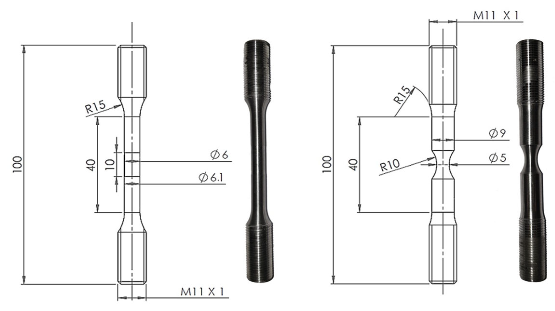
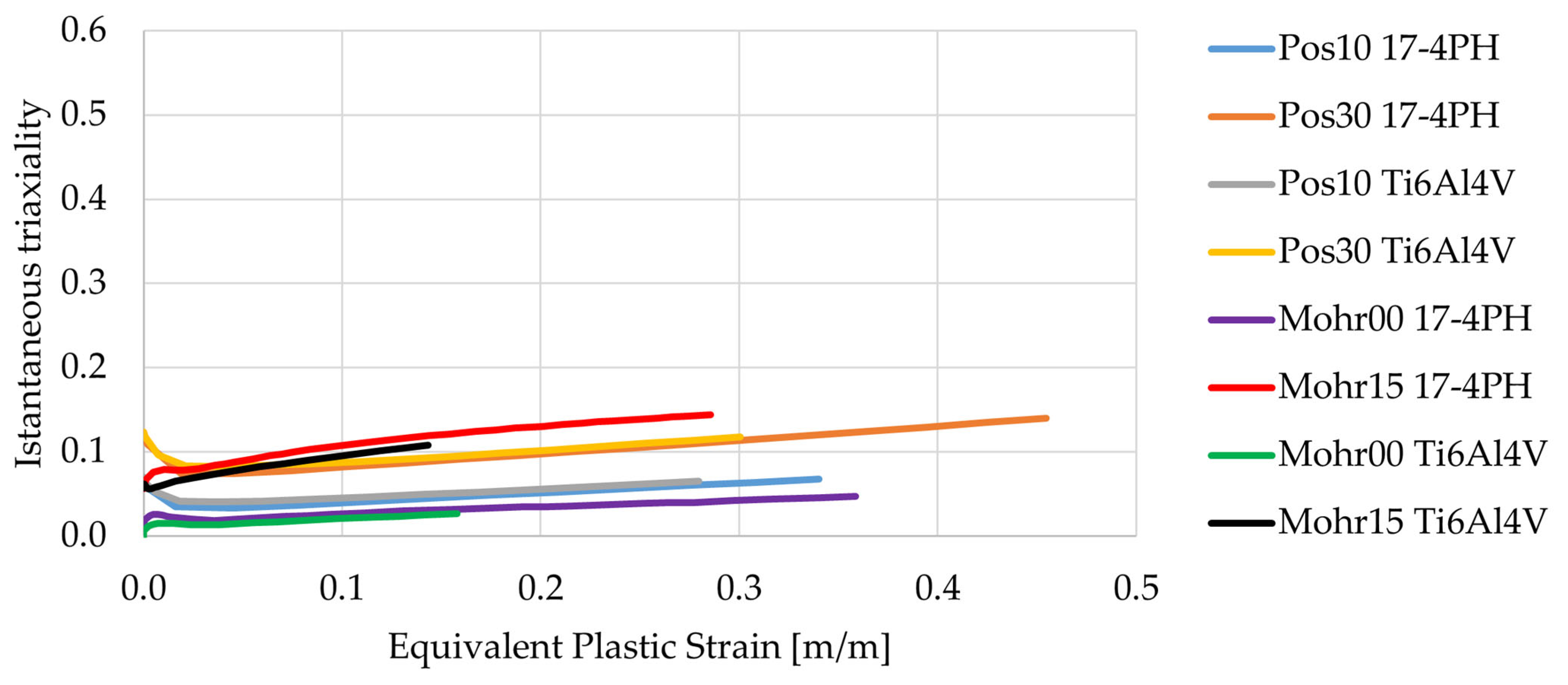
• Driemeier’s specimens (RB, RNB, Pos10, and Pos30);
• Mohr’s specimens (RB, RNB, Mohr00, and Mohr15);
• Driemeier and Mohr’s specimens (RB, RNB, Pos10, Pos30, Mohr00, and Mohr15);
• All tests (RB, RNB, PS, Tors, Pos10, Pos30, Mohr00, and Mohr15).

In particular, the calibration through (1) was used as a reference, being based on conventional tests, while the calibration through (5) relying on the highest number of data is expected to be the most accurate. Once all the calibrations were carried out, a comparison between all the fracture surfaces was put forth to assess the prediction resulting from the different tuning scenarios.

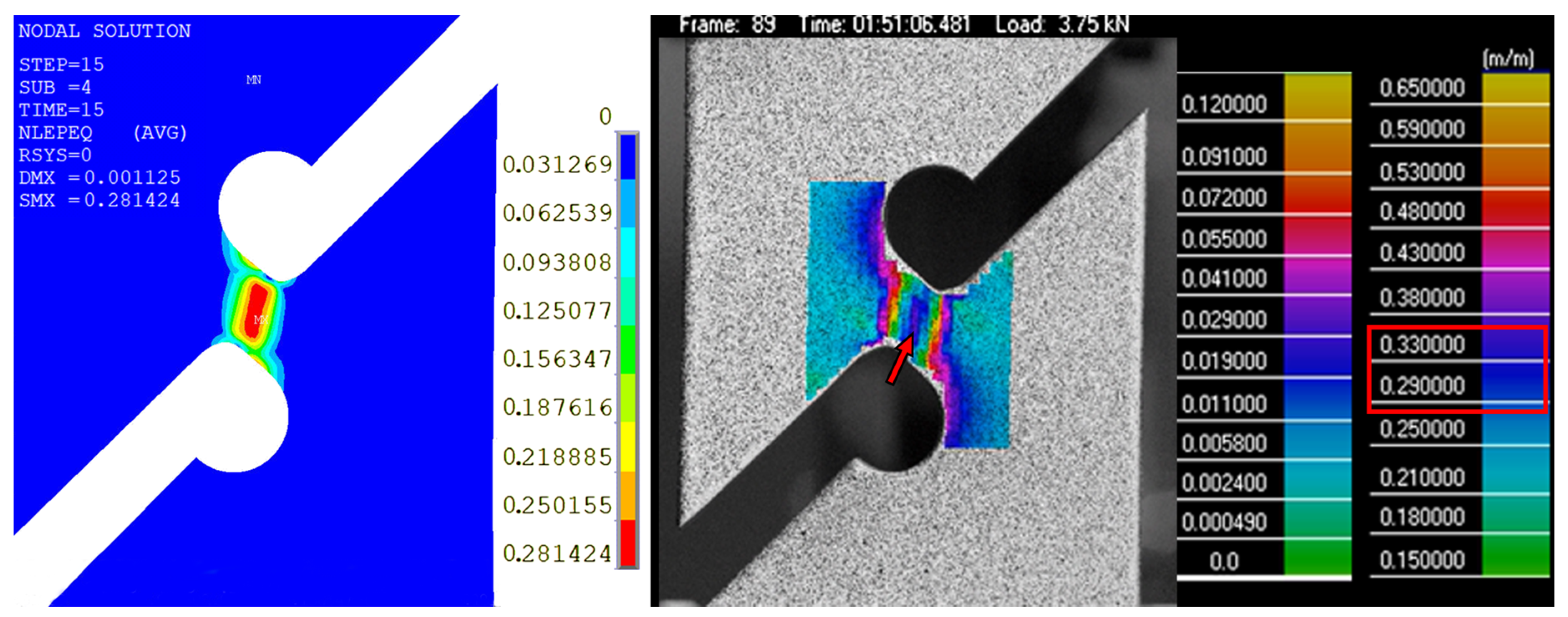
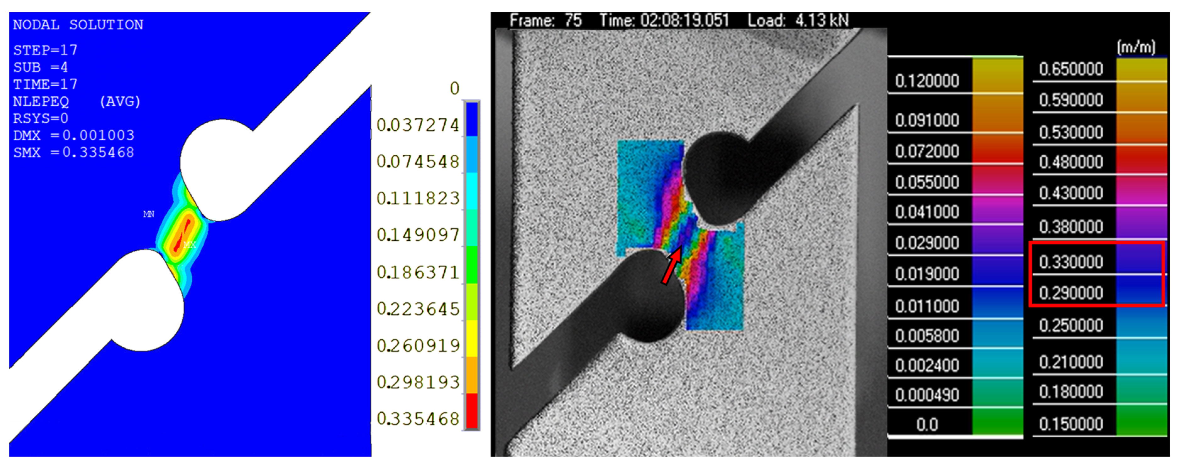
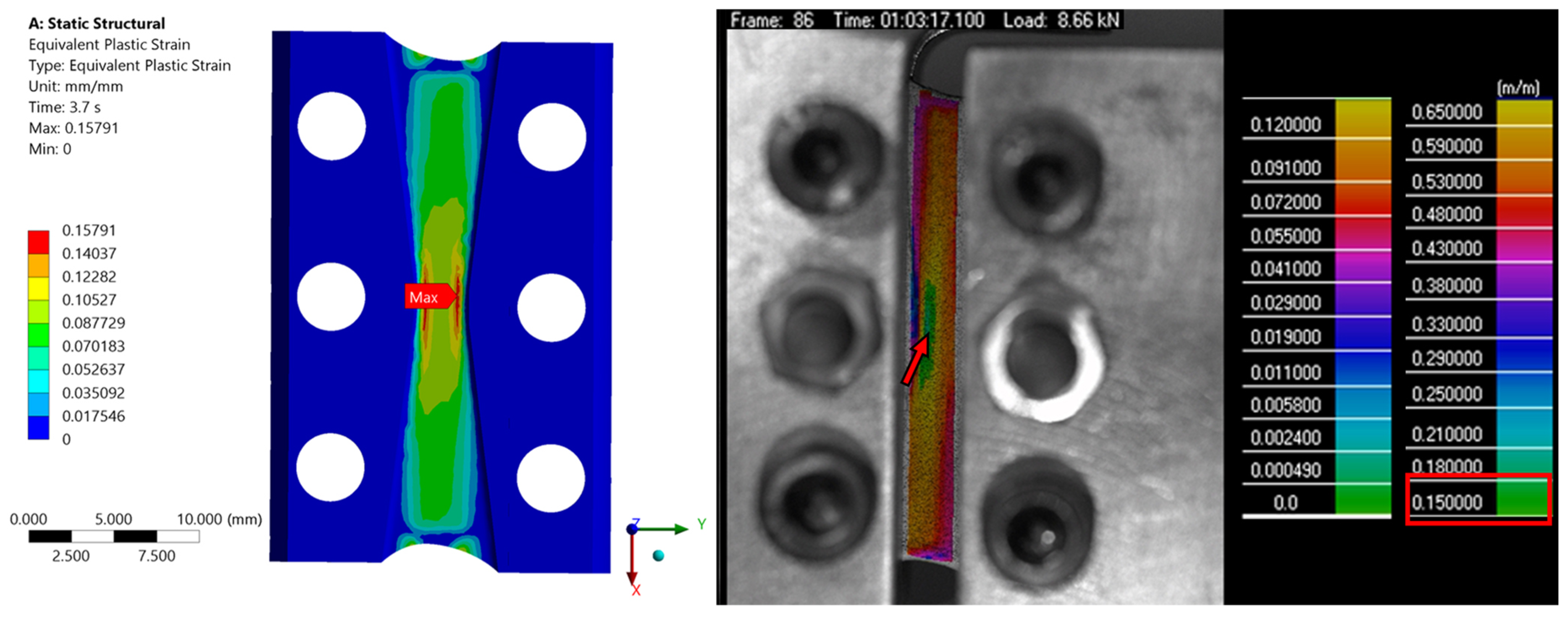
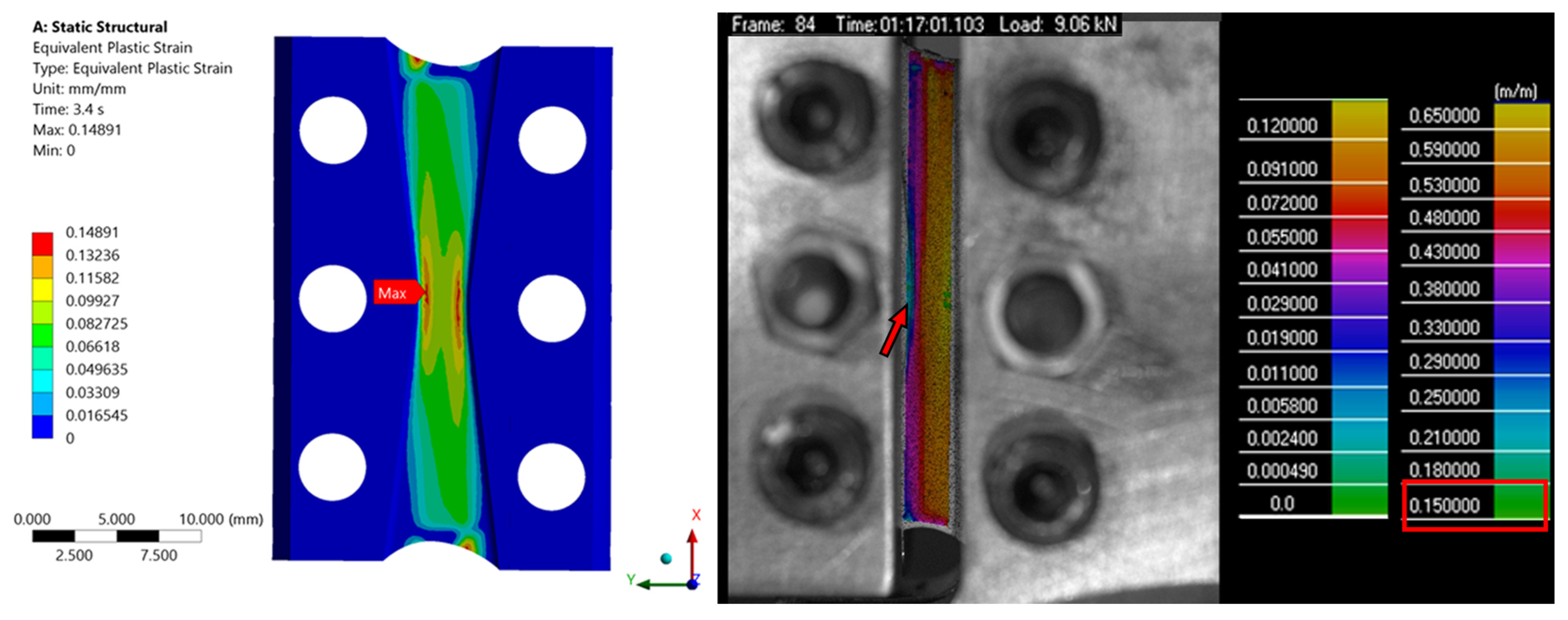
4. Results and Discussion

The main findings are presented in the following order: the results of the experimental campaign, the numerical data extracted from FEA, the outcome of the 2D-DIC analysis, and finally the calibrated fracture surfaces of the different damage models along with a detailed comparison between them.

Figure 7 shows the global load–displacement curves measured experimentally and calculated numerically for the two alloys, with the red dots representing the onset of ductile fracture. Of the three repetitions of each test, for the sake of brevity, only the average experimental values are reported in the figures. As for the global response, the curves obtained experimentally match those obtained via FEA.

For brevity, only the results obtained by DIC-2D relative to instant of fracture of the first repetition for the Driemeier and Mohr’s specimen are shown, for the two materials (Figure 8, Figure 9, Figure 10, Figure 11, Figure 12, Figure 13, Figure 14 and Figure 15). It is worth noting that in all cases, the overall distribution of the equivalent plastic strain obtained via DIC-2D is consistent with that obtained via FEA, with the local values corresponding fairly well. For both specimen types, a central zone of high plastic strain of significant extent is observed, with the deformation decreasing as one moves away from the center. The most critical point of this region, where fracture is expected to occur, is indicated by a red arrow in Figure 8, Figure 9, Figure 10, Figure 11, Figure 12, Figure 13, Figure 14 and Figure 15.

Regarding the results of the Mohr15 specimen obtained via FEM (Figure 11 and Figure 15), a concentration of plastic strain in the external side regions can be observed, with values similar to those present in the central test area; this should not be an issue, however, since the size of this concentration areas is very limited compared to that of the central zone and is furthermore not confirmed by the results obtained via DIC-2D. Therefore, the central zone of the specimen is considered at all effects as the most critical one. The FEM-DIC comparison confirms the accuracy of the FE simulations also from a local standpoint.

Using the FE models, the three principal stresses and the accumulated equivalent plastic strain at the instant of fracture were evaluated at the most critical point of each specimen. From these quantities, the triaxiality parameter T (Equation (2)) and the deviatoric parameter X (Equation (3)) were derived;

Table 1. Average value of triaxiality and deviatoric parameter corresponding to plastic strain at failure in the critical area of all specimens, from FEM.

	Ti6Al4V			17-4PH
Test	${\mathit{T}}_{\mathit{a}\mathit{v}\mathit{g}}$	${\mathit{X}}_{\mathit{a}\mathit{v}\mathit{g}}$	${\mathit{\epsilon }}_{\mathit{f}}$ [m/m]	${\mathit{T}}_{\mathit{a}\mathit{v}\mathit{g}}$	${\mathit{X}}_{\mathit{a}\mathit{v}\mathit{g}}$	${\mathit{\epsilon }}_{\mathit{f}}$ [m/m]
Pos10	0.05	0.18	0.28	0.05	0.16	0.35
Pos30	0.10	0.39	0.30	0.10	0.38	0.46
Mohr00	0.02	0.07	0.16	0.03	0.14	0.35
Mohr15	0.08	0.36	0.15	0.11	0.49	0.28
RB	0.48	0.99	0.63	0.61	0.99	1.17
RNB	0.72	0.99	0.36	0.76	0.99	0.81
PS	0.64	0.00	0.27	0.70	0.00	0.36
Tors	0.00	0.00	0.47	0.00	0.00	0.47

summarizes the local quantities that have been obtained. These data represent the coordinates of specific points in the space (T, X, ${\epsilon }_f$) that are employed as input data in the minimization algorithm of the calibration procedure. The average values T_avg and X_avg calculated via Equations (6) and (7) were assumed, presenting T and X limited variations with plastic strain, as confirmed by the low standard deviation values reported in

Table 2. Standard deviation (Std. dev.) of T and X with respect to the chosen average value $T_{avg}$ and $X_{avg}$.

	Ti6Al4V				17-4PH
	Pos10	Pos30	Mohr00	Mohr15	Pos10	Pos30	Mohr00	Mohr15
Std. dev. T (±)	0.01	0.02	0.01	0.02	0.01	0.02	0.01	0.03
Std. dev. X (±)	0.05	0.07	0.04	0.10	0.05	0.08	0.06	0.11

. This ensures the proportional or quasi proportional hypothesis guaranteeing the validity of Equation (5). The trend of T and X with respect to the accumulated equivalent plastic strain is also reported in Figure 16 and Figure 17. The graphs of the evolution of T and X with plastic strain were plotted on a y axis scaling from 0 to 1, which is the typical range exhibited by these quantities, in order to highlight the quasi-constant evolution.

Table 3. Experimental displacement and load at failure ($d_{exp},F_{exp}$), load at failure resulting from FEM ($F_{FEM}$), plastic strain at failure in the critical area of specimens as retrieved via DIC (${\epsilon }_{f-DIC}$).

	Ti6Al4V				17-4PH
Test	${\mathit{d}}_{\mathit{e}\mathit{x}\mathit{p}}$ [mm]	${\mathit{F}}_{\mathit{e}\mathit{x}\mathit{p}}$ [kN]	${\mathit{F}}_{\mathit{F}\mathit{E}\mathit{M}}$ [kN]	${\mathit{\epsilon }}_{\mathit{f}-\mathit{D}\mathit{I}\mathit{C}}$ [m/m]	${\mathit{d}}_{\mathit{e}\mathit{x}\mathit{p}}$ [mm]	${\mathit{F}}_{\mathit{e}\mathit{x}\mathit{p}}$ [kN]	${\mathit{F}}_{\mathit{F}\mathit{E}\mathit{M}}$ [kN]	${\mathit{\epsilon }}_{\mathit{f}-\mathit{D}\mathit{I}\mathit{C}}$ [m/m]
Pos10	1.00	3.75	3.85	0.32	0.95	3.69	3.70	0.33
Pos30	0.87	4.13	4.23	0.33	0.95	4.08	4.05	0.46
Mohr00	0.74	8.66	8.72	0.16	1.30	8.43	8.54	0.34
Mohr15	0.68	9.06	9.05	0.15	1.05	8.59	8.81	0.30

provides the experimental displacement and load values at failure ($d_{exp},F_{exp}$), the load at failure obtained via FEM ($F_{FEM})$ and the average value of the plastic deformation in the critical zone of the specimen calculated via DIC (${\epsilon }_{f-DIC})$.

The MMC, CC, and HC damage models were calibrated for Ti6Al4V and 17-4PH using data from Table 1, based on the combinations of tests indicated previously. More in detail, the first calibration is performed using only the experimental points of the conventional specimens (RB, RNB, Tors, and PS) and the resulting fracture surface was taken as a reference. The second and third calibrations involved the conventional RB and RNB specimens combined with the Driemeier and Mohr’s multiaxial specimens, respectively. The fourth calibration involved the RB and RNB specimens along with all shear–tension specimens. Finally, in the fifth calibration, data from all experimental tests were used.

To be brief, only the fracture surfaces for Ti6A4V and relative to the three damage models calibrated using the Driemeier and Mohr’s specimens are reported in Figure 18, Figure 19 and Figure 20. In particular, the Driemeier’s fracture surface is shown in Figure 18a, Figure 19a, and Figure 20a, while the Mohr’s fracture surface is shown in Figure 18c, Figure 19c, and Figure 20c. In addition to the 3D graphs, 2D views of ${\epsilon }_f$ behaviour as a function of T_avg for curves at different X_avg are reported in Figure 18b,d, Figure 19b,d, and Figure 20b,d. For completeness, the points related to PS and Tors tests are also included in the graphs, to observe the proximity of the fracture surface to the fracture points relative to the conventional tests. The 3D and 2D views of the fractures surface show a good match with the experimental points employed as input in the minimization algorithm (Equation (9)), showing that each model formulation is well capable of capturing all experimental evidence.

Side-by-side comparisons of the surfaces coming from the different calibrations for the three damage models (MMC, CC, and HC) and for both materials (Ti6Al4V and 17-4PH) are provided in Figure 21. Overall, the five fracture surfaces identified by the different combinations of experimental points are very close to each other. This suggests that no significant differences exist in terms of ductility prediction when a damage model is calibrated through the Driemeier and Mohr’s multiaxial specimens in place of the conventional PS and Tors specimens. The conventional surfaces are slightly higher than the other ones, which is a consequence of the plastic strain values of the PS and Tors tests being higher than those obtained with the multiaxial specimens, though belonging to the same region of the T,X domain. Although the surface obtained with conventional tests was chosen as the reference surface for the comparisons, it is worth a reminder that the surface obtained using all tests should be the most accurate, being based on the largest amount of data. Compared to this last fracture surface, the difference with the Driemeier and Mohr’s calibrated surfaces is even smaller. This further confirms that the selected damage models can be calibrated adopting Driemeier and Mohr’s multiaxial specimens in place of conventional specimens such as PS, Tors, or other multiaxial specimens, with the advantage of using a standard uniaxial testing machine for the experimental phase. Furthermore, regardless of whether the Driemeier or Mohr’s specimens are used, the resulting surfaces are similar in terms of predicted ductility.

It should be noted that for all the proposed combinations, the damage surfaces appear to steepen for low values of triaxiality and values of the deviatoric parameter tending to one. The predicted values of plastic strain at failure by damage surfaces in these zones may provide unreasonable results. The reason lies in the lack of experimental evidence in those areas, namely the unavailability of experimental tests characterized by T and X around 0 and 1 leads to a poor calibration in these areas. Currently, no specimens have been studied in the literature that provide the capability of investigating stress states with these particular T and X values. Surely this problem could represent an interesting opportunity for future studies.

Finally, it is worth noting how each experimental point falls quite close to the evaluated fracture surfaces, which means that either MMC, CC, or HC models are able to predict the plastic deformation at the onset of failure fairly well under very different multiaxial stress states.

Table 4. Calibration constants for TiAl4V alloy and standard deviation errors based on different combinations of inputs for the three damage models. The $n$ parameter for the HC model is set equal to 0.1.

Ti6Al4V	MMC			CC					HC
Test	${\mathit{C}}_1$	${\mathit{C}}_2$	SDErr	${\mathit{C}}_1$	${\mathit{C}}_2$	$\mathit{\beta }$	$\mathit{\gamma }$	SDErr	$\mathit{a}$	$\mathit{b}$	$\mathit{c}$	SDErr
Driemeier	0.079	692.4	0.03	0.82	1.50	0.853	1.000	0.04	1.00	0.80	0.550	0.05
Mohr	0.060	675.0	0.08	0.81	1.55	1.080	1.000	0.03	1.00	0.68	0.020	0.07
Conventional	0.090	710.0	0.09	0.80	1.55	0.997	0.925	0.07	1.10	0.80	0.070	0.04
Driemeier and Mohr	0.060	673.9	0.07	0.81	1.55	1.470	0850	0.07	1.00	0.74	0.036	0.15
All specimens	0.075	689.0	0.11	0.90	1.32	0.840	1.000	0.11	1.00	0.78	0.047	0.11

and

Table 5. Calibration constants for 17-4PH alloy and standard deviation errors based on different combinations of inputs for the three damage models. The $n$ parameter for the HC model is set equal to 0.1.

17-4PH	MMC			CC					HC
Test	${\mathit{C}}_1$	${\mathit{C}}_2$	SDErr	${\mathit{C}}_1$	${\mathit{C}}_2$	$\mathit{\beta }$	$\mathit{\gamma }$	SDErr	$\mathit{a}$	$\mathit{b}$	$\mathit{c}$	SDErr
Driemeier	0.013	742.0	0.14	0.51	1.02	1.970	0.750	0.09	1.02	1.36	0.017	0.12
Mohr	0.013	725.0	0.15	0.50	1.05	1.450	0.990	0.11	1.05	1.10	0.000	0.05
Conventional	0.020	751.0	0.13	0.53	0.85	1.130	0.986	0.11	1.03	1.42	0.020	0.11
Driemeier and Mohr	0.010	721.1	0.12	0.50	1.03	1.240	1.000	0.10	1.00	1.38	0.015	0.20
All specimens	0.020	732.2	0.11	0.60	0.74	1.110	1.000	0.11	1.06	1.20	0.010	0.12

provide the calibration constants for the three damage models and for every material.

5. Conclusions

A simplification of the testing phase required for material ductility evaluation and for ductile damage models calibration was achieved using specific specimen geometries, originally proposed by Driemeier and by Mohr, modified and used to induce multiaxial tensile–shear stress states employing a common uniaxial testing machine as equipment, only. This study showed that the approach can successfully replace more complex and expensive testing normally performed for damage model calibration. An experimental campaign was conducted to test different configurations of the proposed samples on a 17-4PH steel and a Ti6Al4V titanium alloy. Three state-of-the-art ductile damage models were calibrated using conventional tests as well as tests based on Driemeier and Mohr’s specimens. The main findings of this article are summarised below:

▪

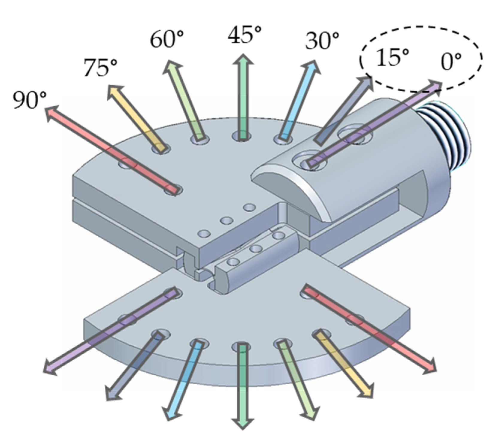
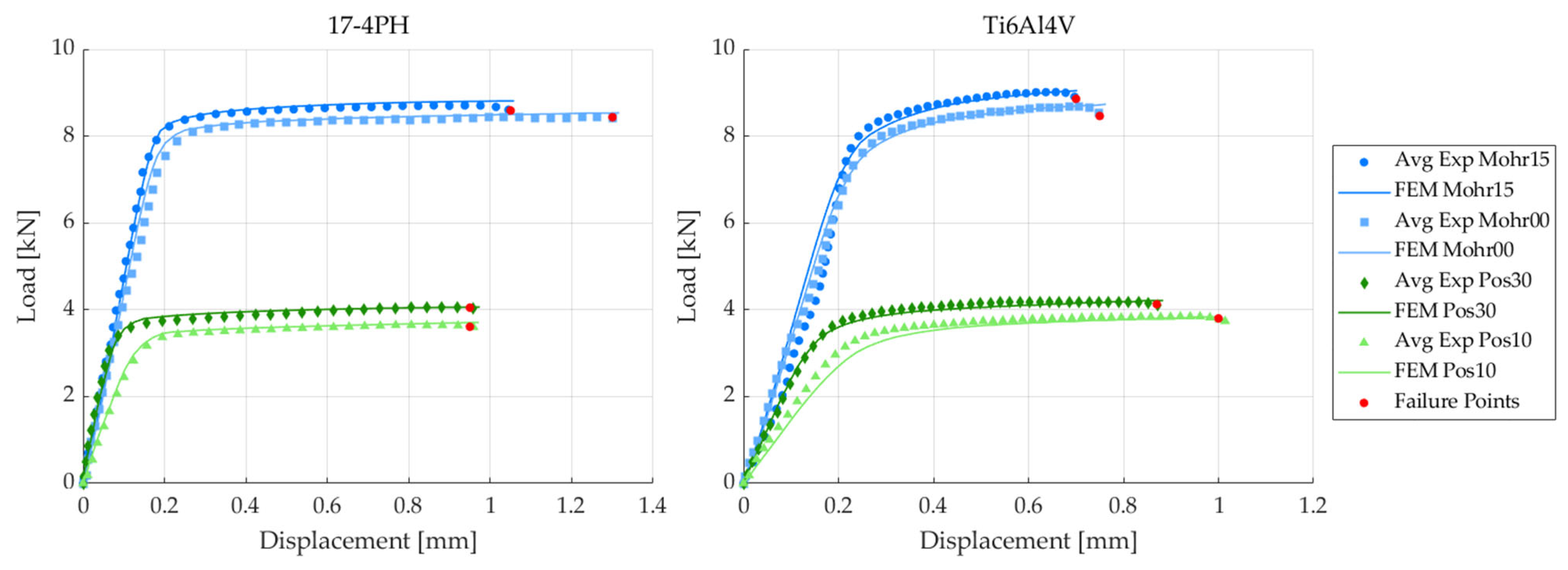
The Driemeier and Mohr’s test specimens are capable of generating several mixed tensile–shear stress states in a low triaxiality regime using only a uniaxial testing machine;

▪

It is possible to vary the tensile-to-shear ratio of the stress state just by changing the machined geometry and dimensions (Driemeier), or just by clamping the samples at a different angle (Mohr) through a purposely designed gripping system;

▪

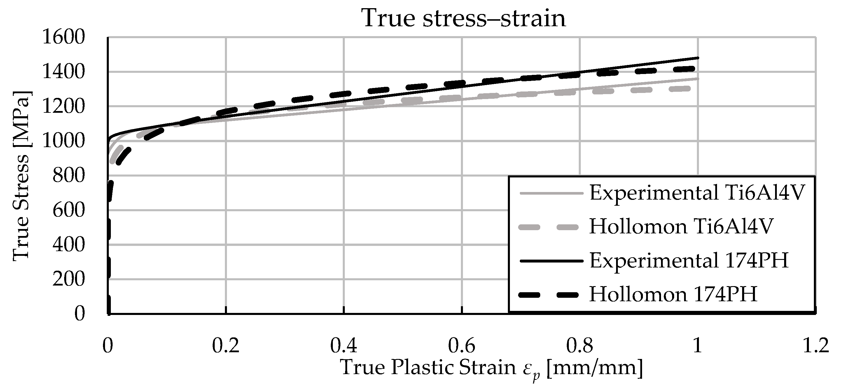
The ductility of a 17-4PH and of a Ti6Al4V alloys could be estimated with the same accuracy level achievable using a more typical complex multiaxial testing and calibration procedure;

▪

The prediction effectiveness of the Modified Mohr–Coulomb, Coppola–Cortese, and Hosford–Coulomb damage models was investigated.

References

1. Vural, H.; Erdogan, C.; Fenercioğlu, T.O.; Yalcinkaya, T. Ductile failure prediction during the flow forming process. Procedia Struct. Integr. 2022, 35, 25–33. [Google Scholar] [CrossRef]
2. Mohamed, M.; Amer, M.; Shazly, M.; Masters, I. Assessment of different ductile damage models of AA5754 for cold forming. Int. J. Adv. Manuf. Technol. 2021, 114, 1219–1231. [Google Scholar] [CrossRef]
3. Behrens, B.-A.; Rosenbusch, D.; Wester, H.; Althaus, P. Comparison of three different ductile damage models for deep drawing simulation of high-strength steels. IOP Conf. Ser. Mater. Sci. Eng. 2022, 1238, 012021. [Google Scholar] [CrossRef]
4. McClintock, F.A. A criterion for ductile fracture by growth of holes. ASME J. Appl. Mech. 1968, 35, 363–371. [Google Scholar] [CrossRef]
5. Rice, J.R.; Tracey, D.M. On the ductile enlargement of voids in triaxial stress fields. J. Mech. Phys. Solids 1969, 17, 201–217. [Google Scholar] [CrossRef]
6. Hancock, J.W.; Mackenzie, A.C. On the mechanism of ductile failure in high-strength steel subjected to multi-axial stresses. J. Mech. Phys. Solids 1976, 24, 147–160. [Google Scholar] [CrossRef]
7. Thomason, P. A three-dimensional model for ductile fracture by the growth and coalescence of microvoids. Acta Metall. 1985, 33, 1087–1095. [Google Scholar] [CrossRef]
8. Rousselier, G. Ductile fracture models and their potential in local approach of fracture. Nucl. Eng. Des. 1987, 105, 97–111. [Google Scholar] [CrossRef]
9. Gurson, A.L. Continuum theory of ductile rupture by void nucleation and growth: Part I Yield criteria and flow rules for porous ductile media. ASME J. Eng. Mater. Technol. 1977, 99, 2–15. [Google Scholar] [CrossRef]
10. Tvergaard, V.; Needleman, A. Analysis of the cup cone fracture in a round tensile bar. Acta Metall. 1984, 32, 157–169. [Google Scholar] [CrossRef]
11. Kachanov, L.M. Time of the rupture process under creep conditions. Izv. Akad. Nauk SSSR Otd. Tekh. Nauk 1958, 8, 26–31. [Google Scholar]
12. Rabotnov, Y.N. Creep Problems in Structural Members; North-Holland Series in Applied Mathematics and Mechanics; North-Holland Pub. Co.: Amsterdam, The Netherlands, 1969; Volume 7, 803p. [Google Scholar]
13. Lemaitre, J. A continuous damage mechanics model for ductile fracture. ASME J. Eng. Mater. Technol. 1985, 107, 83–89. [Google Scholar] [CrossRef]
14. Chaboche, J.-L. Damage induced anisotropy: On the difficulties associated with the active/passive unilateral condition. Int. J. Damage Mech. 1992, 1, 148–171. [Google Scholar] [CrossRef]
15. Chandrakanth, S.; Pandey, P.C. An isotropic damage model for ductile material. Eng. Fract. Mech. 1995, 50, 457–465. [Google Scholar] [CrossRef]
16. Chaboche, J.; Boudifa, M.; Saanouni, K. A CDM approach of ductile damage with plastic compressibility. Int. J. Fract. 2006, 137, 51–75. [Google Scholar] [CrossRef]
17. Zhang, K.; Badreddine, H.; Hfaiedh, N.; Saanouni, K.; Liu, J. Enhanced CDM model accounting of stress triaxiality and Lode angle for ductile damage prediction in metal forming. Int. J. Damage Mech. 2021, 30, 260–282. [Google Scholar] [CrossRef]
18. Bonora, N. A nonlinear CDM model for ductile failure. Eng. Fract. Mech. 1997, 58, 11–28. [Google Scholar] [CrossRef]
19. Bonora, N.; Testa, G. Plasticity damage self-consistent model incorporating stress triaxiality and shear controlled fracture mechanisms—Model formulation. Eng. Fract. Mech. 2022, 271, 108634. [Google Scholar] [CrossRef]
20. Bonora, N.; Testa, G. Plasticity damage self-consistent model incorporating stress triaxiality and shear controlled fracture mechanisms—Model verification and validation. Eng. Fract. Mech. 2022, 271, 108635. [Google Scholar] [CrossRef]
21. Cockcroft, M.G.; Latham, D.J. Ductility and the workability of metals. J. Inst. Met. 1968, 96, 33–39. [Google Scholar]
22. Johnson, G.R.; Cook, W.H. Fracture characteristics of three metals subjected to various strains, strain rates, temperatures and pressures. Eng. Fract. Mech. 1985, 21, 31–48. [Google Scholar] [CrossRef]
23. Bao, Y.; Wierzbicki, T. On fracture locus in the equivalent strain and stress triaxiality space. Int. J. Mech. Sci. 2004, 46, 81–98. [Google Scholar] [CrossRef]
24. Bridgman, P.W. Studies in Large Plastic Flow and Fracture; McGraw-Hill: New York, NY, USA, 1952; p. 177. [Google Scholar] [CrossRef]
25. Gurson, A.L. Plastic Flow and Fracture Behavior of Ductile Materials Incorporating Void Nucleation, Growth and Interaction. Ph.D. Thesis, Brown University, Providence, RI, USA, 1975. [Google Scholar]
26. Bai, Y.; Wierzbicki, T. A new model of metal plasticity and fracture with pressure and Lode dependence. Int. J. Plast. 2008, 24, 1071–1096. [Google Scholar] [CrossRef]
27. Wierzbicki, T.; Bao, Y.; Lee, Y.-W.; Bai, Y. Calibration and evaluation of seven fracture models. Int. J. Mech. Sci. 2005, 47, 719–743. [Google Scholar] [CrossRef]
28. Barsoum, I. Ductile Failure and Rupture Mechanisms in Combined Tension and Shear. Licentiate Thesis No 96 Stockholm. Ph.D. Thesis, KTH Solid Mechanics, Stockholm, Sweden, 2006. [Google Scholar]
29. Coppola, T.; Cortese, L.; Folgarait, P. The effect of stress invariants on ductile fracture limit in steels. Eng. Fract. Mech. 2009, 76, 1288–1302. [Google Scholar] [CrossRef]
30. Mohr, D.; Mercadet, J.S. Micromechanically-motivated phenomenological Hosford-Coulomb model for predicting ductile fracture initiation at low stress triaxialities. Int. J. Solids Struct. 2015, 67–68, 40–55. [Google Scholar] [CrossRef]
31. Lode, W. Versuche über den Einfluß der mittleren Hauptspannung auf das Fließen der Metalle Eisen, Kupfer und Nickel. Z. Phys. 1926, 36, 913–939. [Google Scholar] [CrossRef]
32. Driemeier, L.; Brünig, M.; Micheli, G.; Alves, M. Experiments on stress-triaxiality dependence of material behavior of aluminium alloys. Mech. Mater. 2010, 42, 207–217. [Google Scholar] [CrossRef]
33. Dunand, M.; Mohr, D. Optimized butterfly specimen for the fracture testing of sheet materials under combined normal and shear loading. Eng. Fract. Mech. 2011, 78, 2919–2934. [Google Scholar] [CrossRef]
34. Bai, Y.; Wierzbicki, T. Application of extended Mohr–Coulomb criterion to ductile fracture. Int. J. Fract. 2010, 161, 1–20. [Google Scholar] [CrossRef]
35. Roth, C.C.; Mohr, D. Ductile fracture experiments with locally proportional loading histories. Int. J. Plast. 2016, 79, 328–354. [Google Scholar] [CrossRef]
36. Roth, C.C.; Mohr, D. Effect of strain rate on ductile fracture initiation in advanced high strength steel sheets: Experiments and modeling. Int. J. Plast. 2014, 56, 19–44. [Google Scholar] [CrossRef]
37. Park, S.-J.; Lee, K.; Cerik, B.C.; Choung, J. Ductile fracture prediction of EH36 grade steel based on Hosford–Coulomb model. Ships Offshore Struct. 2019, 14 (Suppl. 1), 219–230. [Google Scholar] [CrossRef]
38. Park, S.-J.; Kim, K. Localized Necking Model for Punching Fracture Simulation in Unstiffened and Stiffened Panels. Appl. Sci. 2021, 11, 3774. [Google Scholar] [CrossRef]
39. Cerik, B.C.; Park, B.; Park, S.-J.; Choung, J. Modeling; testing and calibration of ductile crack formation in grade DH36 ship plates. Mar. Struct. 2019, 66, 27–43. [Google Scholar] [CrossRef]
40. Yu, R.; Li, X.; Yue, Z.; Li, A.; Zhao, Z.; Wang, X.; Zhou, H.; Lu, T.J. Stress state sensitivity for plastic flow and ductile fracture of L907A low-alloy marine steel: From tension to shear. Mater. Sci. Eng. A 2022, 835, 142689. [Google Scholar] [CrossRef]
41. Wilson-Heid, A.E.; Furton, E.T.; Beese, A.M. Contrasting the Role of Pores on the Stress State Dependent Fracture Behavior of Additively Manufactured Low and High Ductility Metals. Materials 2021, 14, 3657. [Google Scholar] [CrossRef]
42. Ma, H.; Qu, R.; Song, K.; Liu, F. Notch strength of ductile materials with different work-hardening behaviors. J. Mater. Res. Technol. 2024, 33, 8974–8982. [Google Scholar] [CrossRef]
43. Olsen, J.S.; Zhang, Z.L.; Lu, H.; Van der Eijk, C. Fracture of notched round-bar NiTi-specimens. Eng. Fract. Mech. 2012, 84, 1–14. [Google Scholar] [CrossRef]
44. Nalli, F.; Imbimbo, B.; Cortese, L. Design of non-conventional biaxial tensile-shear tests for the structural characterization and ductile damage assessment of ductile engineering materials. IOP Conf. Ser. Mater. Sci. Eng. 2021, 1038, 012068. [Google Scholar] [CrossRef]
45. Cortis, G.; Nalli, F.; Piacenti, M. A direct methodology for the calibration of ductile damage models from a simple multiaxial test. IOP Conf. Ser. Mater. Sci. Eng. 2022, 1214, 012016. [Google Scholar] [CrossRef]
46. Moreno-Garibaldi, P.; Alvarez-Vera, M.; Beltrán-Fernández, J.A.; Carrera-Espinoza, R.; Hdz-García, H.M.; Díaz-Guillen, J.C.; Muñoz-Arroyo, R.; Ortega, J.A.; Molenda, P. Characterization of Microstructural and Mechanical Properties of 17-4 PH Stainless Steel by Cold Rolled and Machining vs. DMLS Additive Manufacturing. J. Manuf. Mater. Process. 2024, 8, 48. [Google Scholar] [CrossRef]
47. Shunmugavel, M.; Polishetty, A.; Littlefair, G. Microstructure and Mechanical Properties of Wrought and Additive Manufactured Ti-6Al-4V Cylindrical. Procedia Technol. 2015, 20, 231–236. [Google Scholar] [CrossRef]
48. Cortis, G.; Broggiato, G.B.; Cortese, L. Ductility assessment of a 17-4PH steel through simple multiaxial tests. In Proceedings of the 2023 IOP Conference Series: Materials Science and Engineering, Padova, Italy, 7–10 September 2022. [Google Scholar] [CrossRef]
49. Nalli, F.; Cortese, L.; Concli, F. Ductile damage assessment of Ti6Al4V, 17-4PH and AlSi10Mg for additive manufacturing. Eng. Fract. Mech. 2021, 241, 107395. [Google Scholar] [CrossRef]
50. Cortese, L.; Nalli, F.; Broggiato, G.B.; Coppola, T. An effective experimental-numerical procedure for damage assessment of Ti6Al4V. In Residual Stress, Thermomechanics & Infrared Imaging, Hybrid Techniques and Inverse Problems, Volume 9, Proceedings of the 2015 Annual Conference on Experimental and Applied Mechanics, Costa Mesa, CA, USA, 8–11 June 2015; Bossuyt, S., Schajer, G., Carpinteri, A., Eds.; Conference Proceedings of the Society for Experimental Mechanics Series (CPSEMS); Springer: Cham, Switzerland, 2016. [Google Scholar] [CrossRef]
Figure 1. Round bar (RB) specimen and round notched bar (RNB) specimen.
Applsci 15 03645 g001
Figure 2. (a) Technical drawing of Driemeier’s specimen with detail for α = 10° (Pos10) and α = 30° (Pos30) configurations; (b) machined sample for Pos10 configuration.
Applsci 15 03645 g002
Figure 3. Mohr’s specimen: (a) technical drawing; (b) machined sample.
Applsci 15 03645 g003
Figure 4. Mohr’s specimen: clamping system to be connected to the test machine grips by screw connections. All seven possible pulling directions are reported, with the loading direction used at 0° (Mohr00) and 15° (Mohr15) highlighted by dashed circle.
Applsci 15 03645 g004
Figure 5. 17-4PH and Ti6Al4V experimental stress–strain curves, with corresponding power law fit. The maximum value of 1.0 is conventionally chosen and represents the nominal true plastic strain.
Applsci 15 03645 g005
Figure 6. Mesh size, applied displacements, and constraints for the Driemeier and Mohr’s specimens. For the Mohr’s sample, the pulling directions that were actually tested (0°, 15°) are reported.
Applsci 15 03645 g006
Figure 7. Experimental and numerical load–displacement curves for 17-4PH and Ti6Al4V alloys. The red dots indicate the onset of plastic failure.
Applsci 15 03645 g007
Figure 8. FEM-DIC comparison using Ansys Mechanical APDL for Driemeier Pos10, Ti6Al4V. The area of fracture is indicated by a red arrow, while in the legend the red box indicates the critical value of plastic strain to failure. The same applies to the following figures.
Applsci 15 03645 g008
Figure 9. FEM-DIC comparison using Ansys Mechanical APDL for Driemeier Pos30, Ti6Al4V.
Applsci 15 03645 g009
Figure 10. FEM-DIC comparison using Ansys Workbench for Mohr00, Ti6Al4V.
Applsci 15 03645 g010
Figure 11. FEM-DIC comparison using Ansys Workbench for Mohr15, Ti6Al4V.
Applsci 15 03645 g011
Figure 12. FEM-DIC comparison using Ansys Mechanical APDL for Driemeier Pos10, 17-4PH.
Applsci 15 03645 g012
Figure 13. FEM-DIC comparison using Ansys Mechanical APDL for Driemeier Pos30, 17-4PH.
Applsci 15 03645 g013
Figure 14. FEM-DIC comparison using Ansys Workbench for Mohr00, 17-4PH.
Applsci 15 03645 g014
Figure 15. FEM-DIC comparison using Ansys Workbench for Mohr15, 17-4PH.
Applsci 15 03645 g015
Figure 16. Evolution of triaxiality T with respect to equivalent plastic strain.
Applsci 15 03645 g016
Figure 17. Evolution of deviatoric parameter X with respect to equivalent plastic strain.
Applsci 15 03645 g017
Figure 18. Ti6Al4V fracture surface calibrated through Driemeier and Mohr’s tests, MMC model: (a) 3D fracture surface calibrated using Driemeier specimens plus RB and RNB; (b) 2D view of fracture surfaces for Driemeier surface; (c) 3D fracture surface calibrated using Mohr specimens plus RB and RNB; (d) 2D view of fracture surfaces for Mohr surface.
Applsci 15 03645 g018
Figure 19. Ti6Al4V fracture surface calibrated through Driemeier and Mohr’s tests, CC model: (a) 3D fracture surface calibrated using Driemeier specimens plus RB and RNB; (b) 2D view of fracture surfaces for Driemeier surface; (c) 3D fracture surface calibrated using Mohr specimens plus RB and RNB; (d) 2D view of fracture surfaces for Mohr surface.
Applsci 15 03645 g019aApplsci 15 03645 g019b
Figure 20. Ti6Al4V fracture surface calibrated through Driemeier and Mohr’s tests, HC model: (a) 3D fracture surface calibrated using Driemeier specimens plus RB and RNB; (b) 2D view of fracture surfaces for Driemeier surface; (c) 3D fracture surface calibrated using Mohr specimens plus RB and RNB; (d) 2D view of fracture surfaces for Mohr surface.
Applsci 15 03645 g020
Figure 21. Comparison of Ti6Al4V and 17-4PH fracture surfaces coming from calibrations using different combinations of tests (1–5, see the list at the end or materials and methods section) for the three damage models. Fracture surfaces of: (a) Ti6Al4V for MMC model; (b) 17-4PH for MMC model; (c) Ti6Al4V for CC model; (d) 17-4PH for CC model; (e) Ti6Al4V for HC model; (f) 17-4PH for HC model.
Applsci 15 03645 g021aApplsci 15 03645 g021b