Article

Optimizing Police Patrol Strategies in Real-World Scenarios: A Modified PPS-MOEA/D Approach for Constrained Multi-Objective Optimization

1
School of Information Network Security, People’s Public Security University of China, Beijing 100038, China
2
School of Criminology, People’s Public Security University of China, Beijing 100038, China
3
School of Computer and Artificial Intelligence, Beijing Technology and Business University, Beijing 100048, China
*
Author to whom correspondence should be addressed.
Appl. Sci. 2025, 15(7), 3651; https://doi.org/10.3390/app15073651
Submission received: 20 February 2025 / Revised: 24 March 2025 / Accepted: 25 March 2025 / Published: 26 March 2025

Abstract

:
This study addresses the realistic constrained multi-objective optimization problem of police patrols by constructing a mathematical model tailored to the actual operational context of police patrols in China. To solve this problem, a modified PPS-MOEA/D algorithm is proposed and its performance is systematically evaluated against several state-of-the-art Constrained Multi-Objective Evolutionary Algorithms (CMOEAs). The results demonstrate the superiority of the proposed approach in terms of the solution quality and computational efficiency. Furthermore, the optimal solution set is discussed and visualized on a map, providing decision makers with practical and actionable insights that align with real-world patrol requirements. This research not only advances the theoretical framework for police patrol optimization, but also offers a practical tool for enhancing the effectiveness and efficiency of law enforcement operations in urban environments.

1. Introduction

Police patrol strategies have been extensively studied and empirically demonstrated to significantly reduce crime rates while enhancing public perceptions of security, thereby constituting a critical operational focus for frontline law enforcement agencies [1]. In China, police deployment predominantly relies on the 110 call for the police service platform, which allocates the nearest available units based on reported incidents [2]. However, this reactive policing model falls short of meeting the evolving societal demands for security and the heightened expectations for proactive police services. Consequently, transitioning to an active policing paradigm has emerged as an imperative reform, aiming to optimize police resource allocation and enable timely interventions at potential risk sites [3]. A central challenge in this transition lies in determining the optimal spatial distribution of patrol units to ensure rapid response capabilities while minimizing resource inefficiencies. Fundamentally, this challenge represents a quintessential multi-objective optimization problem, balancing competing priorities such as the response time, resource utilization, and crime prevention efficacy.
Currently, there are still significant challenges in applying multi-objective optimization methods to solve the Police Patrol Optimization Problem (PPOP). As illustrated in Figure 1, PPOP is supposed to determine optimal patrol routes for police units. The solution aims to achieve three key objectives: (1) ensuring a rapid response to incidents by prioritizing the coverage of nearby streets [4,5], (2) maximizing the probability of police presence on main streets to enhance visibility [6,7], and (3) minimizing the time spent transitioning between streets to improve the operational efficiency and allocate more time to active patrolling or incident management [8,9]. These objectives often present inherent trade-offs, necessitating a delicate balance to formulate an effective and practical solution. Moreover, real-world constraints—such as geographical limitations, resource availability, and dynamic conditions like traffic congestion [10,11]—introduce significant layers of complexity. These factors not only complicate the optimization process, but also amplify the challenge of developing strategies that are both efficient and adaptable to changing environments.
Traditional multi-objective optimization algorithms often underperform in handling constraint conditions, failing to fully meet the diverse requirements of actual patrol tasks, particularly in dynamically changing environments where their adaptability is limited. Additionally, many existing methods exhibit deficiencies in global search efficiency, leading to the suboptimal convergence and robustness of solutions. These shortcomings become especially evident when tackling large-scale optimization problems, defined here as scenarios involving hundreds of patrol streets, and high-dimensional optimization problems, characterized by three or more conflicting objectives and constraints.
To address these issues, this paper proposes a method based on the PPS-MOEA/D (Push and Pull Search + Multi-Objective Evolutionary Algorithm based on Decomposition). This approach leverages the efficient convergence of the PPS algorithm [12] and the decomposition strategy advantages of MOEA/D [13], enabling the effective balancing of multi-objective optimization under complex constraint conditions. Simulation validation was carried out using real-world data from a subdistrict in Chaoyang, Beijing.

2. Related Work

The practical value of PPOP have been extensively validated through numerous studies [14,15,16]. At its core, the central decision-making challenge in the police patrol optimization problem lies in the optimal deployment of limited law enforcement resources to critical positions, ensuring the swiftest possible response to potential incidents [17]. Recent research on PPOP has explored various methodologies, which can be broadly categorized into single-objective optimization and multi-objective optimization approaches. This section systematically reviews these approaches, highlighting their methodologies, advantages, and limitations.

2.1. Single-Objective Optimization Approaches

Single-objective optimization focuses on optimizing a single criterion, such as resource allocation, the response time, or crime coverage. For example, Basilico et al. introduced Patrolling Security Games (PSGs), modeling strategic patrolling as extensive-form infinite-horizon games [18]. Chen et al. proposed a patrol strategy combining the ant colony algorithm with Bayesian decision making, focusing on optimizing local decisions [19]. Johanna Leigh et al. developed an algorithm that maximizes the coverage of high-crime areas [20]. Wu et al. applied game theory to PPOP, focusing on minimizing deployment costs based on risk values derived from the Nash equilibrium [21]. Chase et al. developed the GRAND-VISION patrol scheduling system, which uses mixed-integer programming to optimize resource allocation across regions and time periods [22]. Chainey et al. designed patrol paths based on static historical crime data, focusing solely on maximizing the coverage of crime hotspots [23]. Guevara et al. proposed a smart patrol system that integrates machine learning with real-time crime predictions, focusing solely on maximizing crime coverage [24].
Despite their promising efforts, the aforementioned single-objective optimization approaches—incorporating game theory, mathematical programming, machine learning, and heuristic algorithms—exhibit notable limitations. For instance, Basilico et al.’s [18] PSGs lack scalability for multiple patrollers and empirical validation. Chen et al.’s [19] greedy strategy does not guarantee global optimality. Johanna Leigh et al.’s [20] algorithm fails to guarantee optimal solutions in complex scenarios. Wu et al.’s [21] method does not address practical patrol path generation. Chase et al.’s [22] approach neglects patrol route optimization. Chainey et al.’s [23] reliance on static historical crime data limits their system’s ability to handle dynamic environments. Guevara et al.’s [24] system relies on simplistic linear regression for crime predictions, limiting its accuracy. More broadly, these methods often depend on static data or overly simplistic models, constraining their effectiveness in dynamic and complex environments. Their narrow focus on single objectives frequently results in suboptimal solutions when multiple objectives need to be balanced simultaneously. Given that real-world patrol tasks inherently involve trade-offs among competing objectives, the inherent constraints of single-objective approaches underscore the necessity for more comprehensive frameworks capable of addressing multiple objectives effectively.

2.2. Multi-Objective Optimization Approaches

Compared to the single-objective optimization of police patrols, multi-objective optimization addresses the need to balance multiple conflicting criteria simultaneously, providing more comprehensive solutions to the PPOP. For instance, Wang et al. employed Integer Programming (IP) to balance street coverage and minimize police deployment, introducing a decomposition approach to handle the NP-hard nature of the problem [25]. Subsequently, Wang et al. extended their approach to a two-stage CSP framework, incorporating both offline and real-time patrol models to maximize incident service rates [26], later adapting it for traffic security patrols under frequency constraints [27]. Joe et al. employed reinforcement learning (RL) to tackle dynamic patrol scheduling, focusing on two optimization objectives: maximizing the success rate of the incident response and minimizing patrol presence reduction [28]. They later extended this model to multi-agent cooperative scenarios, leveraging RL’s strength in achieving global optimization [29]. Jiang et al. proposed a genetic algorithm-based method to optimize street patrol routes, aiming to minimize the response time and reduce the number of patrol inspectors [30].
Despite their advancements, these multi-objective optimization methods exhibit significant limitations. Wang et al.’s [25,26,27] approaches, while theoretically robust, face challenges with scalability and real-time applicability. Joe et al.’s [28,29] RL-based method, though effective in dual-objective optimization, essentially reduces the problem to a single-objective formulation through its reward function, limiting its ability to fully capture the trade-offs between competing goals. Jiang et al.’s [30] genetic algorithm assigns fixed weights to objectives, which fails to qualify as a true multi-objective optimization approach, and its reliance on static crime data constrains its effectiveness in dynamic environments. More broadly, existing methods struggle to achieve genuine constrained multi-objective optimization in intricate environments. They are often limited by scalability issues, the inability to balance competing objectives adequately, and reliance on static or simplistic models, which hinder their applicability in dynamic and multi-patrol scenarios. These limitations underscore the need for more efficient algorithms capable of addressing the complexities of patrol pathing and resource allocation in real-world settings.
In recent years, Multi-Objective Evolutionary Algorithms (MOEAs) have demonstrated a remarkable performance in solving multi-objective optimization problems [31]. Numerous notable algorithms have emerged, such as NSGA-II [32], NSGA-III [33], SPEA2 [34], MOEA/D [35], IBEA [36], and HypE [37], which have significantly advanced the field. Notably, Constrained Multi-Objective Evolutionary Algorithms (CMOEAs) have effectively addressed optimization challenges by incorporating mechanisms specifically designed to handle constraints efficiently [38], including innovative algorithms like I-DBEA [39], ShiP [40], and BiCo [41]. Furthermore, the Push–Pull Search (PPS) algorithm offers distinct advantages, such as an enhanced convergence speed and adaptability to complex search landscapes, making it particularly suitable for dynamic and intricate optimization scenarios [42,43].
Leveraging these advancements, this paper proposes the integration of the PPS-MOEA/D algorithm to tackle the complex and dynamic challenges inherent in PPOP, including resource allocation, route planning, and constraint satisfaction. This approach aims to provide a more robust and efficient solution to the multifaceted problems encountered in real-world patrol operations, ultimately improving the effectiveness and adaptability of patrol strategies.

3. Model Formulation

The primary objective of this study focuses on addressing the PPOP by determining optimal deployment strategies for patrol units within an urban street network. Specifically, the research aims to establish the operational trajectory for each patrol unit across distinct temporal intervals from 08:00 to 23:00 on a designated day. The focus on this time frame is justified by empirical data analysis, which indicates that the majority of incidents occur within this period, with a substantial decrease in street incidents between 00:00 and 07:00 when most people are typically at rest. This optimization process is conducted under real-world constraints, with the fundamental decision variable being the allocation of the patrol unit, p n   , to a specific street, s i , during the time period, T . The comprehensive patrol scheme is designed to simultaneously satisfy three critical optimization criteria: (1) the maximization of 110 incident risk coverage, (2) the maximization of the police visibility rate, and (3) the minimization of the inter-street transfer time. This multi-objective optimization framework ensures an efficient and effective patrol strategy that addresses key operational requirements in urban security management.

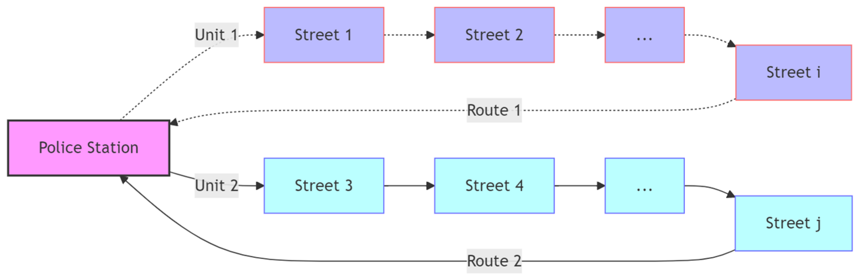
3.1. Problem Definition

Graph theory offers a strong modeling framework for urban street networks, treating streets as nodes and distances as edges to capture spatial relationships and the urban structure. This approach facilitates the application of graph algorithms to optimize patrol routes, reduce transition times, and efficiently allocate resources, which is especially advantageous for PPOP due to its dynamic and scalable nature.
The PPOP can be formally defined as follows: Consider a network of m streets, G , within a given jurisdiction, where n officer units, P = p 1 , p 2 , . . . , p n (typically deployed in pairs), are responsible for executing daily patrol operations over a specified time horizon, T (e.g., from 08:00 to 23:00, comprising 16 one-hour intervals). Each officer unit is required to patrol distinct streets during consecutive time intervals, necessitating transitions between street assignments at each time step.
To enhance temporal resolution in patrol scheduling, we introduce a fine-tuning parameter δ = 1,2 , 3 that governs the granularity of time intervals. When δ = 1 (default setting), the total time horizon T = 1,2 , . . . , 16 , with each interval representing a 60 min patrol duration. For δ = 2 , T = 1,2 , . . . , 32 , corresponding to 30 min patrol intervals. When δ = 3 , T = 1,2 , . . . , 48 , resulting in 20 min patrol intervals. For computational simplicity, the duration of each patrol interval inherently includes the transition time between consecutive street assignments, where transition time optimization constitutes a key objective for future research.
The street network within the district is formally represented as G = S , D , L , R , where:
S = s 1 , s 2 , . . . , s m denotes the set of m streets in the network.
D represents the weight matrix of the network, where d i j corresponds to the traveling distance between any pair of streets
L = l 1 , l 2 , . . . , l m denotes the length of each street.
R = r 1 t , r 2 t , . . . , r m t represents the risk of 110 call incidents on each street at hour t , which is derived from a deep spatio-temporal graph attention network [44]. It is important to note that the street risk values are hour-based due to the temporal granularity of the data. Consequently, when the fine-tuning parameter δ is set to 2,3 , the risk value remains constant over the corresponding two or three consecutive patrol intervals.
The binary decision variable x B m t is defined over the Cartesian product of m streets and t patrol time intervals, where x i t indicates the patrol assignment for street i at time interval t . Specifically, x i t = 1 if street i is selected for patrol during time interval t , and x i t = 0 otherwise.

3.2. Objective Function

The PPOP primarily involves three key objectives.
Objective 1: Maximization of Risk Coverage
The first objective is to maximize the total risk coverage, defined as the sum of risk values across all patrolled streets during the day. For instance, if two officer units are assigned to complete patrol tasks over 16 h, the goal is to maximize the sum of risk values across the 2 × 16 = 32 patrolled streets. This objective ensures that limited police resources are allocated to the streets with the highest risk, thereby achieving optimal risk coverage. This approach aligns with the principles of hotspot policing, which emphasizes focusing resources on high-risk areas to enhance public safety [45,46,47].
M a x i m i z e   o b j e c t i v e 1 = i = 1 m t = 1 T x i t · r i t
Objective 2: Maximization of Total Patrolled Street Length
The second objective is to maximize the total length of all patrolled streets during the day. For example, if two officer units are assigned to complete patrol tasks over 16 h, the goal is to maximize the sum of the lengths of the 2 × 16 = 32 patrolled streets. This objective aims to achieve the highest possible police visibility by ensuring that officers cover the greatest cumulative distance across the street network. Maximizing the total patrolled length enhances the perceived presence of law enforcement, which can deter potential criminal activities and improve public safety [48,49].
M a x i m i z e   o b j e c t i v e 2 = i = 1 m t = 1 T x i t · l i  
Objective 3: Minimization of Transfer Time Between Streets
The third objective is to minimize the transfer time between streets during patrols, thereby reducing unnecessary inefficiencies in resource allocation. Intuitively, when an officer unit transitions from the current street to the next, the nearest street (i.e., the one requiring the least travel time) should be selected from the available options. This minimizes the time wasted on necessary transitions, optimizing the utilization of police resources. Let x i j t p denote the decision variable, indicating that officer unit p transitions from street i to street j at the end of time interval t , with this process continuing until the final transition is completed at time interval T 1 .
M i n i m i z e   o b j e c t i v e 3 = p = 1 n t = 1 T 1 x i j t p · d i j
Multi-Objective Optimization
The three objectives described above may exhibit certain trade-offs or conflicts in specific scenarios. However, for police patrol operations, it is desirable to simultaneously satisfy all three objectives. To facilitate the optimization process, the first two objectives (the maximization of risk coverage and maximization of the total patrolled street length) can be transformed into minimization problems by taking their reciprocals, while the third objective remains unchanged.
f 1 ( x ) = 1 / o b j e c t i v e 1 f 2 ( x ) = 1 / o b j e c t i v e 2 f 3 ( x ) = o b j e c t i v e 3
Therefore, the three-objective optimization problem can be formulated as:
M i n i m i z e   F x = f 1 x , f 2 x , f 3 x T

3.3. Constraints

The optimization problem is subject to the following constraints:
Patrol Assignment Constraint:
Ensure that in each time interval t , all n officer units are assigned to n distinct streets for patrol:
i = 1 m x i t = n   t 1,2 , . . . , T
Transition Constraint:
Ensure that each officer unit transitions to a different street for patrol in the next time interval, preventing units from remaining on the same street continuously. This constraint enhances the efficiency and motivation of police patrol work:
p = 1 n t x i j t p = p = 1 n t + 1 x i j t p   i j
Starting Street Constraint:
Ensure that all officer units start their patrol from a designated starting street s 0   :
x i 0 = s 0
Ending Street Constraint:
Ensure that all officer teams return to the designated starting street s 0 at the end of the patrol period:
x i T + 1 = s 0
Risk Coverage Constraint:
Ensure that the total risk coverage across all patrolled streets is at least equal to the average risk value:
i = 1 m t = 1 T x i t · r i t i t R i t m × T × n
Street Length Coverage Constraint:
Ensure that the total length of all patrolled streets is at least equal to the average length of all streets:
i = 1 m t = 1 T x i t · l i i L i m × n
Transfer Time Constraint:
Ensure that the average time required for all necessary street transitions is less than or equal to 10 min. This ensures that even in extreme cases (e.g., δ = 3 ) each street is patrolled for at least 10 min. According to statistical data from the Amap platform, the average driving distance within a 10 min interval on urban road networks, such as those in Beijing, is approximately 3–5 km. This empirical observation provides a practical basis for setting the transfer time constraint in the police patrol optimization model.
p = 1 n t = 1 T 1 x i j t p · d i j n × T 1 × 3000
Exploration of Diverse Streets
To ensure that the patrol routes cover a diverse range of streets within the limited patrol time and enhance the exploratory nature of the model, we introduce a binary variable z i . When z i = 1 , street i is visited more than once during the whole patrol period, otherwise z i = 0 .
i ( 1 z i ) i t x i t θ
where θ is a predefined threshold that limits the proportion of streets that can be revisited. This constraint encourages the patrol routes to explore new streets rather than repeatedly visiting the same ones, thereby maximizing the coverage of the street network. The parameter θ is set to a default value of 0.5, which signifies that a minimum of 50% of the streets should remain non-repeatedly visited during the patrol cycles, ensuring sufficient coverage and diversity in the patrol routes.
Coverage of Historically High-Risk Streets
To ensure that the patrol routes prioritize streets with a history of incidents, we introduce a binary variable h i . When h i = 1 , street i has a history of real incidents, otherwise h i = 0 .
i t x i t · h i i t x i t μ
where μ is a predefined threshold that ensures the proportion of historically high-risk streets among all patrolled streets is above a certain level. The parameter μ is set to a default value of 0.3. This threshold is determined based on statistical analysis, as out of the total 390 streets, only 129 have historically recorded incidents, accounting for less than 30% of the total street count. This constraint guarantees that the patrol routes focus on areas with a higher likelihood of incidents, aligning with the principles of proactive policing.

4. Algorithm Implementation

To address the constrained multi-objective optimization in the PPOP, this study proposes an integrated model combining deep-network-based risk predictions with a modified PPS-MOEA/D algorithm. The framework primarily consists of two key components: risk prediction and path optimization. Initially, a deep spatio-temporal graph attention network (DSTGAT) is employed to generate hourly risk predictions for all street networks within the study area, providing essential intelligence guidance for subsequent path planning. The emphasis of this paper lies in the implementation of the optimization algorithm; thus, the architectural details and implementation specifics of the deep learning prediction algorithm can be seen in another work [50].
Owing to the numerous realistic constraints inherent in our research task, the PPS-MOEA/D framework was selected to address the constraint-handling mechanism, which is specifically divided into push and pull phases. During the push phase, the population’s search and convergence processes disregard constraint limitations, allowing traversal through infeasible regions while simultaneously mapping the constraint landscape. In the subsequent pull phase, the algorithm leverages the information gathered during the push phase to guide parameter settings, thereby enhancing adaptability. The core philosophy of MOEA/D lies in decomposing the multi-objective optimization problem into multiple single-objective subproblems, utilizing a neighborhood search mechanism to maintain population diversity and optimize efficiency. Through the implementation of uniformly distributed weight vectors and localized searches within neighborhoods, MOEA/D efficiently approximates the Pareto front while maintaining a balance between global and local search capabilities. Consequently, these methods are integrated to tackle the constrained multi-objective optimization problem, with empirical evidence demonstrating their efficacy. However, the raw codes cannot be directly applied to the practical problem under investigation in this study, necessitating substantial modifications to achieve the predefined objectives. The corresponding flowchart is presented in Figure 2.

4.1. Initialization

As illustrated in Figure 2, the first step of the algorithm is to initialize the relevant system parameters. This includes randomly generating an initial population and computing the values of the three objective functions as well as the constraints. Additionally, the weight vectors are initialized according to the requirements of the MOEA/D algorithm. Most of the initialization tasks and the calculations of the objective functions and constraints can be directly performed using the functions defined in the model. However, two critical aspects warrant emphasis: the first is initial population generation, and the second is the calculation of the third objective function.
The generation of the initial population must adhere to the constraint conditions, specifically ensuring that for each time step t , there are exactly n elements with a value of 1, while the remaining elements are set to 0, as stipulated by Constraint 1.
To achieve the goal of minimizing the transfer time (i.e., Objective 3), two techniques are employed. The diagonal elements of the original distance matrix D are set to positive infinity (inf). This ensures that during the transfer process, the patrol unit does not select the current street for the next time step, thereby preventing stationary patrols and promoting the continuous movement of police forces. This design aligns with the requirements of Constraint 2.
The second technique employs the Munkres algorithm (also known as the Hungarian algorithm [40]), a classical method for solving assignment problems. Its primary objective is to identify the optimal task allocation scheme within a given cost matrix, minimizing the total cost. The core principle of the algorithm involves row reduction, column reduction, and matrix adjustment to iteratively determine the optimal matching. Renowned for its efficiency and precision, the Munkres algorithm is particularly well-suited for scenarios requiring a globally optimal solution.
In the context of the transfer process, multiple patrol units need to select the nearest streets to patrol based on their current locations. To illustrate this, consider Figure 3: assuming initialization has resulted in the selection of four streets out of ten for patrol over three time steps, the assignment of different units to distinct routes between adjacent time steps to achieve the shortest global distance constitutes a classic matching problem. The Munkres algorithm is instrumental in resolving this issue, ensuring an optimal assignment of patrol routes across time steps.
The process begins by extracting submatrices from the initial distance matrix based on the streets selected in adjacent time steps. For instance, using the streets selected at t = 1 and t = 2 , the corresponding distance submatrix is derived, as presented in Table 1.
Next, the submatrix undergoes a row reduction step according to the Munkres algorithm, where each row is subtracted by its minimum value, resulting in the transformed matrix shown in Table 2.
Following this, a column reduction step is performed, where each column is subtracted by its minimum value, yielding the transformed matrix presented in Table 3.
In the transformed submatrix, elements with a value of zero represent potential assignment streets. The algorithm begins by identifying the first uncovered zero in the first row and marks it with an asterisk (*) to indicate a potential assignment. The column containing this marked zero is then covered to prevent redundant assignments. This process is repeated for subsequent rows, searching for uncovered zeros and marking them while covering their respective columns, until all rows have been processed.
The algorithm then counts the total number of covered rows and columns. If the sum of covered rows and columns equals the number of rows (or columns) in the matrix, the algorithm terminates, and the marked asterisk elements represent the optimal assignment solution. However, if the total number of covered rows and columns is less than the number of rows, the remaining matrix undergoes further row and column reduction steps, followed by the marking and covering process, until the assignment is fully resolved.
Based on Table 3, the optimal assignment results are determined as follows: 1→4, 2→5, 3→7, and 4→6, with a total transfer distance of 3000 + 3000 + 4000 + 2000 = 12,000.
Subsequently, the same procedure is applied to the second and third rows of Figure 3, yielding the following results: 4→8, 5→6, 6→7, and 7→9. By connecting these optimal assignment results with lines, the patrol paths are generated, as illustrated in Figure 4.
Therefore, by computing Objective 3, the dual goals of minimizing the transfer time and enhancing the efficiency of police patrol operations are achieved. Additionally, this approach generates optimal patrol paths for each group, demonstrating a clever design in this study.

4.2. Differential Evolution

Based on a predefined probability, two individuals are randomly selected from either the neighborhood of each individual or the entire population, forming a set of three individuals. These individuals are then subjected to mutation according to the Differential Evolution (DE) algorithm [51] to generate new offspring. Since the offspring produced by DE are randomly generated, they may violate the constraints defined in the model. For instance, the number of “1”s in a certain row might exceed or fall short of the number of patrol units, n . To address this issue, a repair mechanism is introduced in this study. Specifically, if the number of “1”s exceeds n , the excess “1”s are randomly removed; if the number of “1”s is less than n , the missing “1”s are randomly added.

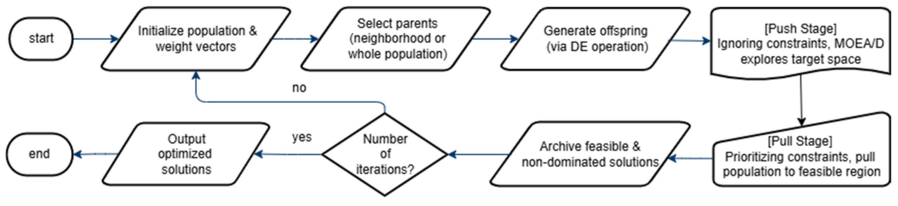
4.3. Push and Pull Phases

The transition between the Push and Pull phases can be achieved either by manually setting the population update generations or by introducing parameters for dynamic switching. This dynamic switching mechanism can automatically adjust the search strategy based on the optimization state of the population, thereby achieving a better balance between global exploration and a local search.
During the Push phase, the algorithm ignores the constraint conditions and leverages the efficient optimization capabilities of the MOEA/D algorithm. By decomposing the multi-objective optimization problem into multiple subproblems and employing a neighborhood search mechanism, the algorithm accelerates the convergence of the population. This design enables the algorithm to rapidly explore the search space without considering constraints, thereby providing a well-initialized population for the subsequent Pull phase.
In the Pull phase, the algorithm first introduces a constraint handling mechanism to gradually guide infeasible solutions into feasible regions. Additionally, a dynamic adjustment strategy is implemented, allowing the algorithm to adapt more flexibly to varying constraints and objectives.

4.4. Preservation of Feasible Non-Dominated Solutions

Finally, the program identifies individuals from the population that satisfy the constraint conditions and sorts them according to the non-dominated sorting principle. The complete set of feasible solutions is then output as the final result.

5. Simulation Settings

The proposed algorithm was applied to the jurisdiction of the DT sub-district in the Chaoyang District, Beijing, China, located in the northwestern part of the district with an area of approximately 10 square kilometers. In 2019, the permanent population of the area was about 132,457. This study focused on the street network within the jurisdiction, with data sourced from OpenStreetMap (OSM), totaling 390 streets. The DT sub-district was chosen for this simulation due to its high levels of population, economic activity, area size, and police incident frequency within the Chaoyang District, making it a representative case study.

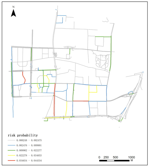
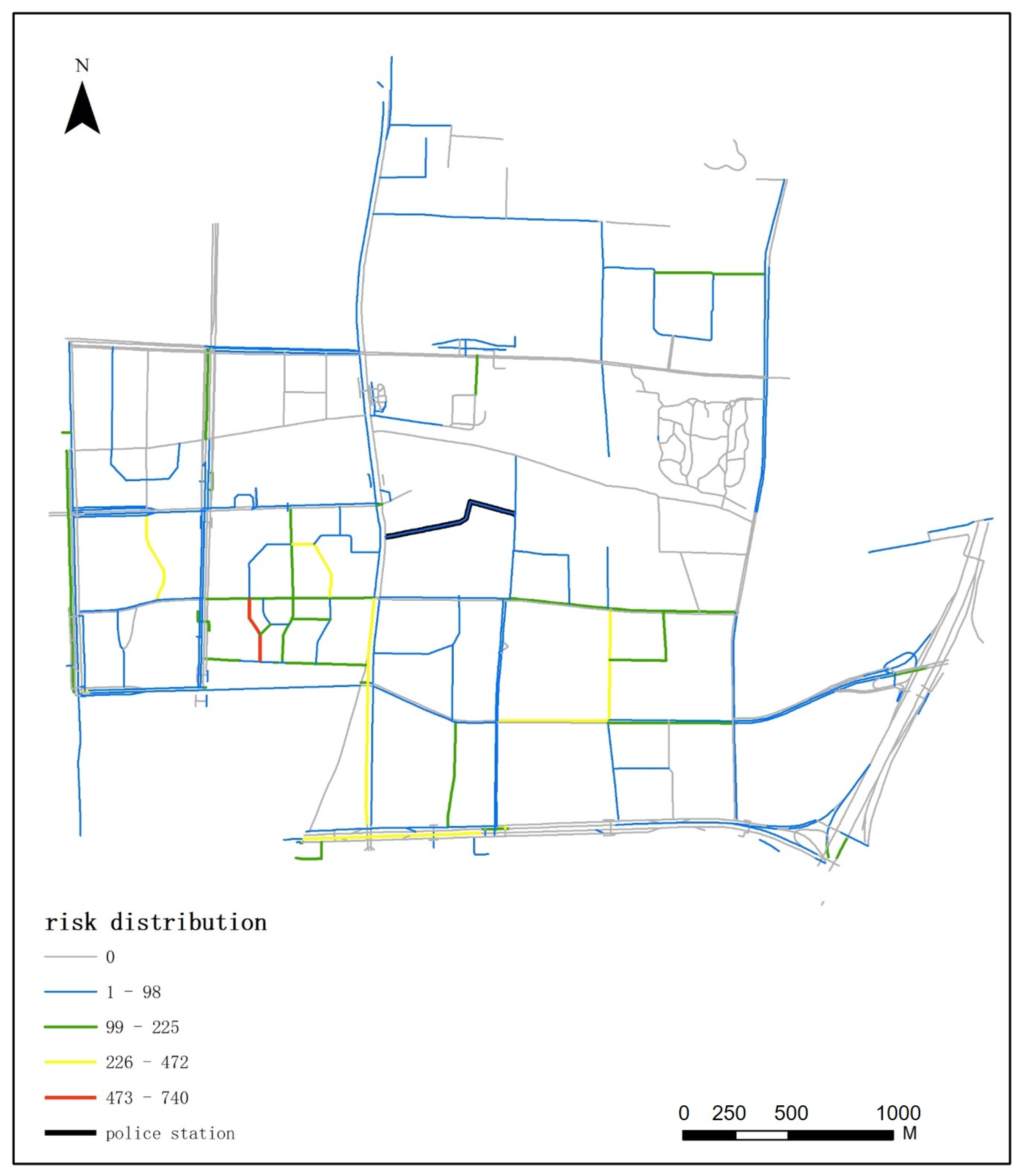
5.1. 110 Incident Risk Distribution

In 2019, the police department corresponding to the DT sub-district received a total of 10,625 incident reports, each of which included both temporal and spatial information. To associate these incident reports with their respective streets, the Nearest Neighbor Algorithm was implemented in ArcGIS. The spatial distribution of 110 incident risks across the entire year of 2019 is illustrated in Figure 5.
It is important to note that the 110 incident risk exhibits dynamic changes over time. By conducting hourly statistical analysis, these temporal variations can be effectively observed. The changes in the 110 incident risk between 16:00 and 23:00 are clearly illustrated in Appendix A, providing a comprehensive visualization of the temporal dynamics.
If the generation of patrol route schemes fails to account for the time-varying characteristics of the 110 incident risk, the resulting solutions would clearly be suboptimal. Therefore, this study incorporates these dynamic variations as a critical input into the optimization algorithm, integrating them into Objective Function 1 for computational purposes.

5.2. Street Length and Distance Matrix

The street network data, sourced from OpenStreetMap (OSM), includes essential information such as the street length, which is utilized for the calculation of Objective Function 2.
The distance matrix serves as a fundamental dataset for the entire algorithm. To address the challenge of real-time path planning in response to dynamic traffic conditions, this study employs the Amap Driving Route Planning API to efficiently generate the real-time shortest paths between streets. This approach ensures the algorithm’s adaptability to real-world traffic variations.

5.3. Baseline Algorithms and Parameter Settings

To validate the effectiveness of the proposed algorithm, seven constrained multi-objective optimization algorithms were introduced for comparison: CTAEA [52], CCMO [53], CMOES [54], MFOSPEA2 [55], MOEADDAE [56], NSGAII [32], and ANSGAIII [33].
The parameter settings are as follows:
Population size (N): 100.
Number of objectives (M): three.
Number of neighbors (T): 10.
Differential evolution parameters: crossover rate (CR) = 0.5, scaling factor (f) = 0.5.
Probability of selecting individuals from neighbors (\delta): 0.9.
Stopping criterion: each algorithm was independently executed 30 times, with the number of function evaluations reaching 300,000 per run.

5.4. Performance Metrics

To evaluate the performance of different algorithms, this study employs two commonly used metrics in multi-objective optimization: Hypervolume (HV) and Spacing (SP).
Hypervolume (HV) is a widely adopted metric that measures both the convergence and diversity of the solution set in the objective space [57]. A higher HV value indicates a more optimal and comprehensive set of solutions. In this study, HV is calculated using the following formula:
H V S = 1 n i = 1 n V O L x S f 1 x , z 1 r × f m x , z m r
In the HV calculation, V O L · represents the Lebesgue measure, which is used to quantify the volume in the objective space formed between each solution and the reference point. Here, z m r denotes the reference point defined by the user in the objective space. It is important to note that in this study, the HV is calculated as the mean value rather than the cumulative sum of the HV across all solution sets. This adjustment is necessary because different algorithms may produce varying numbers of solutions, and the use of the mean ensures a fair comparison across algorithms.
Since the problem under investigation is a real-world scenario, there is no known true Pareto front available. Therefore, the choice of the reference point becomes critical for comparing the performance of different algorithms. To address this, the reference point is determined through preliminary experiments. Specifically, the maximum values across all objectives achieved by the solution sets of all algorithms are identified, and an offset (e.g., 1.1 times these maximum values) is added to ensure the reference point is sufficiently large to encompass all solutions. This approach guarantees that the HV is computed under the same reference point for all algorithms, thereby ensuring the fairness and reliability of the comparison.
To provide a comprehensive evaluation of the algorithm performance and mitigate the limitations of relying solely on a single metric, this study introduces an additional metric: Spacing (SP). This metric is employed to assess the uniformity of the distribution of solutions in the objective space [58]. A smaller SP value indicates a more evenly distributed solution set, which is typically preferred as it suggests a more diverse set of solutions. However, the ’optimal’ SP value can vary depending on the specific objectives of the study and the balance between exploration and exploitation. Our aim is to identify SP values that ensure a balanced distribution of solutions, promoting both diversity and quality in the solution set. The SP metric is calculated using the following formula:
s p a c i n g S = 1 n 1 i = 1 n m i n j i d x i , x j
where d x i , x j represents the Euclidean distance between solutions x i and x j .
Furthermore, since this study addresses a constrained multi-objective optimization problem, a third metric is introduced: the number of feasible solutions. This metric counts the solutions in the final population that satisfy all constraints. This metric is particularly important as it directly reflects an algorithm’s ability to generate feasible solutions under constraints.

5.5. Hardware and Platform

The Inspur (Beijing, China) server used for the simulation is equipped with a 32-core processor CPU, 128 GB RAM, and A100 GPU.
The PlatEMO (Platform for Evolutionary Multi-objective Optimization) framework, a widely recognized and open-source MATLAB -based platform designed for multi-objective optimization algorithms, was utilized [59]. PlatEMO provides a robust and standardized environment for implementing, testing, and benchmarking optimization algorithms. In this study, PlatEMO v4.9 was employed, running on MATLAB R2023a.

6. Simulation Results

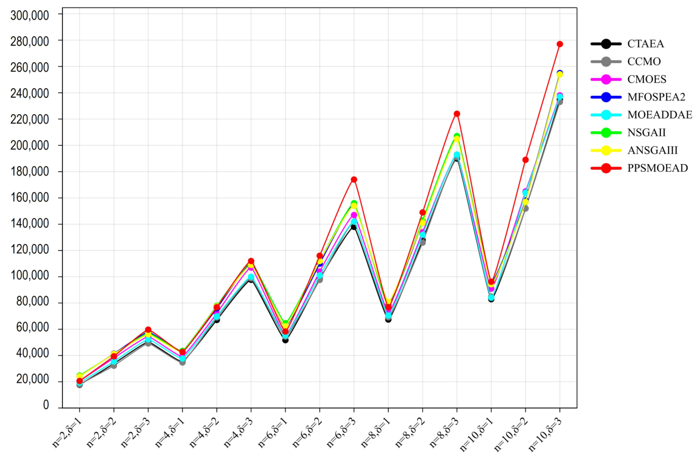
6.1. Comparative Analysis

To evaluate the performance of various algorithms under different scenarios, simulations were conducted by introducing two key parameters defined in the model: the number of patrol units, n = 2,4 , 6,8 , 10 , and the time parameter, δ = 1,2 , 3 .
This resulted in a total of 15 combinatorial scenarios. The final simulation results are presented in Figure 6, Figure 7 and Figure 8, which provide a detailed comparison of the algorithms based on the performance metrics. For a more detailed presentation of the simulation results, please refer to Appendix B.1, Appendix B.2 and Appendix B.3.
From the results presented in Figure 6, it is evident that the modified PPS-MOEA/D algorithm outperformed all other comparative algorithms in solving the proposed police patrol problem. Specifically, in all 15 scenarios, the modified PPS-MOEA/D achieved superior Hypervolume (HV) values, demonstrating its exceptional capability in terms of convergence and diversity for this specific optimization task.
The algorithms ANSGA-III and NSGA-II ranked second and third, respectively, based on their HV performance. This indicates that these NSGA-based algorithms consistently exhibit a strong performance in practical optimization problems, reaffirming their robustness and effectiveness.
The dominance of the modified PPS-MOEA/D highlights its adaptability and efficiency in addressing the unique challenges of the police patrol problem, while the consistent performance of ANSGA-III and NSGA-II underscores the reliability of NSGA-based approaches in multi-objective optimization.
Building on the comparison of the Hypervolume (HV) metric, Figure 7 provides insights into the Spacing metric, which evaluates the distribution uniformity of solutions in the Pareto front. Meanwhile, the modified PPS-MOEA/D algorithm outperforms the other algorithms across most scenarios.
Furthermore, although the CCMO algorithm demonstrates a slightly better Spacing performance compared to the modified PPS-MOEA/D, its performance is highly unstable, as observed in Figure 7, which illustrates this inconsistency. The CTAEA algorithm ranks third, as stable, demonstrating a moderate performance in terms of solution distribution uniformity.
These observations underscore the importance of critically interpreting performance metrics and highlight the modified PPS-MOEA/D as a robust and reliable algorithm for achieving a well-distributed Pareto front in the PPOP.
As illustrated in Figure 8, most algorithms, excluding MOEA/D-DAE, are capable of generating a significant number of feasible solutions. Among these, the PPS-MOEA/D, NSGA-II, and ANSGA-III algorithms exhibit the most stable and consistent performance, further reinforcing their efficacy in addressing the proposed police patrol problem.
In summary, the PPS-MOEA/D algorithm demonstrates the best overall performance in solving the police patrol optimization problem, as evidenced by its superior results across multiple evaluation metrics.

6.2. Optimization Objectives Comparison

The core focus of this study lies in the optimization of three key objectives: maximizing risk coverage and the longest street length, and minimizing the transition distance.
To evaluate the performance of different algorithms, the mean values of these objectives were compared. Notably, the first two objective values were inverted to align with the real-world context of maximizing risk coverage and minimizing the longest street length, respectively. This approach ensures that the results are directly interpretable in the context of the practical problem being addressed.
Figure 9 presents the average risk coverage values of patrol routes obtained by different algorithms across various scenarios. Each cell in the table represents the mean value of the risk coverage achieved by the respective algorithm for a specific scenario. The risk coverage metric reflects the ability of a patrol route to effectively encompass areas with higher incident risk, demonstrating the performance of each algorithm in addressing dynamic risk conditions.
Figure 10 displays the average total street length of patrol routes generated by different algorithms across various scenarios. Each cell in the table represents the mean value of the summed street lengths covered by the respective algorithm for a particular scenario. A higher value indicates a greater street-level police presence, reflecting improved visibility and accessibility of law enforcement in the patrolled area. This metric serves as a critical indicator of the effectiveness of each algorithm in maximizing street coverage, thereby enhancing public safety and reassurance.
Figure 11 presents the average total transfer distance of patrol routes generated by different algorithms across various scenarios. Each cell in the table represents the mean value of the summed transfer distances computed by the respective algorithm for a specific scenario. A lower value indicates a reduction in non-productive (“ineffective”) transfer distances, signifying improved efficiency in the allocation of police resources to active patrol tasks. Minimizing the transfer distance is crucial for optimizing the operational efficiency, as it ensures that a larger proportion of police time and effort is dedicated to actual policing activities rather than unnecessary movement between locations.
Based on the results presented in Figure 9, Figure 10 and Figure 11, which compare the performance of algorithms across the three optimization objectives, the PPS-MOEA/D algorithm maintains a dominant position overall. Although a few algorithms achieve slight superiority in certain scenarios for the first two objectives, PPS-MOEA/D consistently delivers a robust and superior performance across the majority of cases.

7. Discussion

This section primarily discusses how the three objective optimization values can be applied to the daily patrol operations of law enforcement agencies. Specifically, decision makers can make an optimal selection for implementation based on real-world conditions, such as the availability of police personnel, the granularity of the patrol time (whether long or short), and other relevant factors, using the solutions provided by the approach.

7.1. Trends and Insights

Appendix B.4, Appendix B.5 and Appendix B.6 present the optimization results of the three objectives obtained using the proposed method under different scenarios. Based on Figure 12 and Figure 13, the overall trend of changes can be further analyzed, providing valuable insights.
Figure 12 presents a comparative analysis of the global cumulative results. Overall, as the number of patrol units increases and the patrol intervals are further segmented, both risk coverage and the patrolled street length exhibit a significant upward trend. However, the transfer distance also increases correspondingly, partially offsetting these benefits.
Figure 13 further illustrates that with an increasing number of patrol units and the finer segmentation of patrol intervals, the efficiency of individual units per time interval generally declines. This trend is most pronounced in risk coverage, while the impact on the patrolled street length is less significant. The transfer distance, on the other hand, initially decreases significantly, but then stabilizes or even increases when δ = 1 .
Based on the above analysis, the following recommendations can be provided for decision makers.
First, deploying a minimum of n = 2 or a maximum of n = 10 patrol units is not highly recommended. A small number of units fail to cover sufficient risk areas, whereas an excessive number of units leads to a decline in operational efficiency.
Secondly, from the perspective of balancing efficiency and risk coverage, the following two scenarios are recommended: n = 6 and δ = 2 or n = 8 and δ = 2 . The rationale is as follows: the overall risk coverage is relatively high (1.3539 for the former and 1.6690 for the latter), and the average risk coverage is also satisfactory (0.0047 for the former and 0.0043 for the latter). Additionally, the total transfer distance remains acceptable compared to high-risk coverage scenarios (469,950 for the former and 610,580 for the latter). Both scenarios are suitable for decision makers seeking high patrol efficiency while avoiding excessive transfer distances.
Thirdly, from the perspective of minimizing the transfer distance while maintaining a relatively high risk coverage, the following two scenarios are recommended: n = 4 , δ = 1 or n = 6 , δ = 1 . The rationale is that while the overall risk coverage is not the highest, it remains reasonable (0.7026 for the former and 0.9179 for the latter). More importantly, the total transfer distance is significantly lower than other high-risk coverage scenarios (131,940 for the former and 195,220 for the latter), and the average transfer distance is among the lowest (1434.13 for the former and 1414.64 for the latter). Both scenarios are suitable for decision makers who need to consider transfer costs while maintaining a reasonable level of risk coverage.

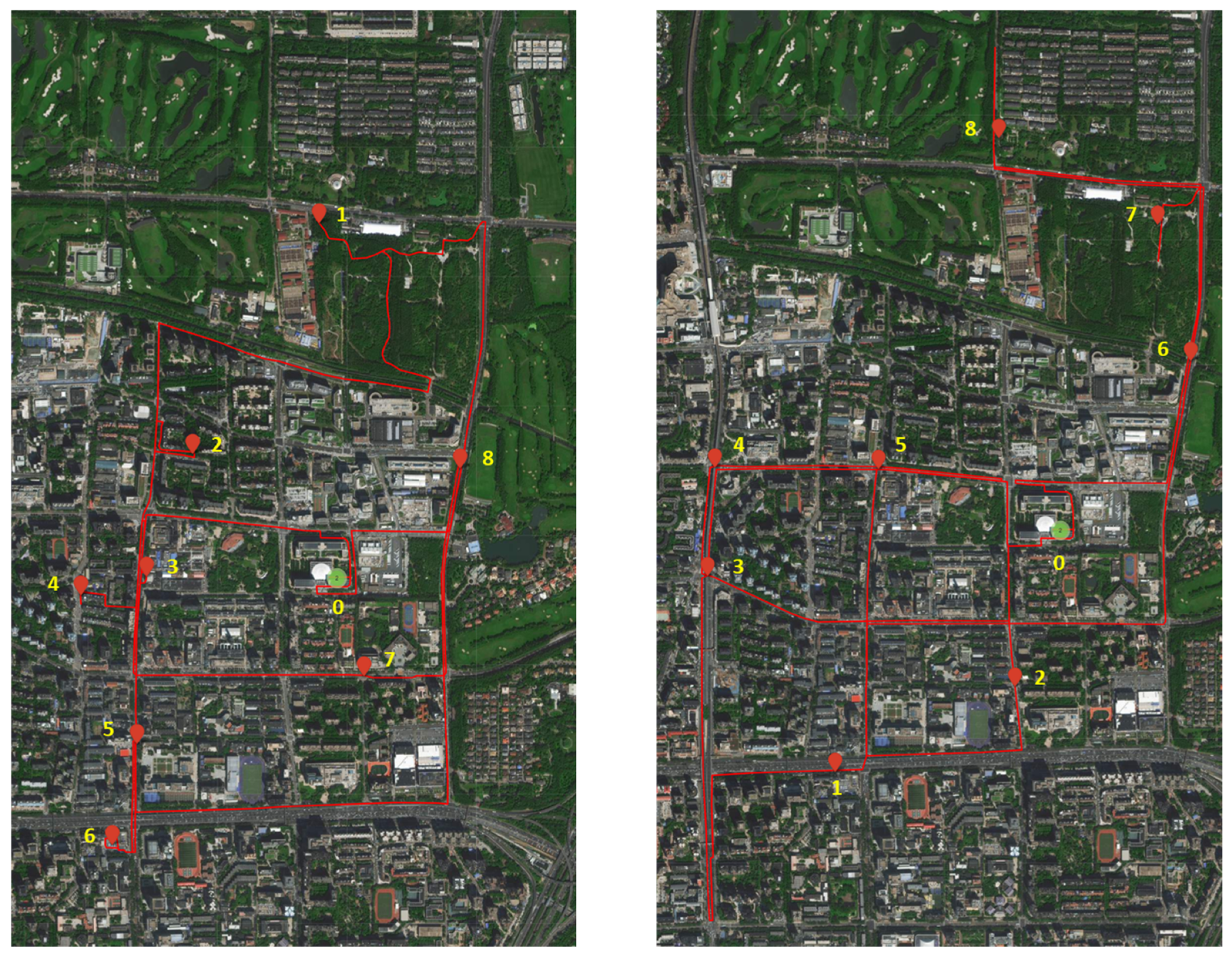
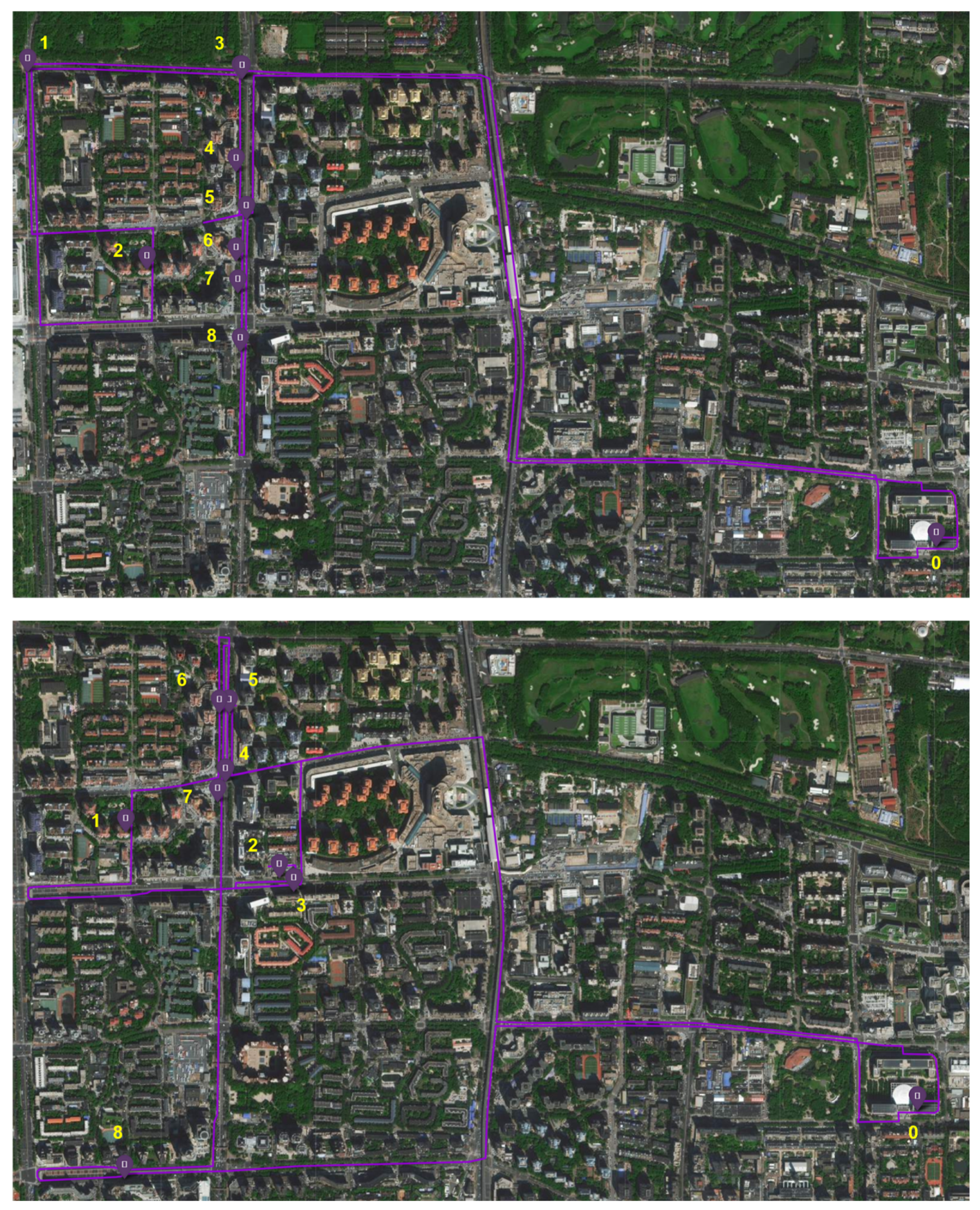
7.2. Visualization of Optimal Solutions

The ultimate goal of this study is to obtain the optimal police patrol routes under various scenario combinations. Based on the simulation results, we selected a specific scenario (e.g., n = 4 , δ = 1 ) and illustrate eight patrol routes from the feasible solutions obtained by the PPS-MOEA/D algorithm. The patrol period spans from 08:00 to 23:00, totaling 16 h, which is divided into two shifts: the first shift at 08:00–15:00, and the second shift at 16:00–23:00. Each shift begins and ends at the police station, ensuring that the patrol tasks are completed within the designated time frames. The patrol routes are generated in real-time based on the route planning API provided by Amap. By integrating this real-time routing capability into the patrol optimization framework, the system ensures that the generated routes are practical, adaptable, and responsive to the dynamic nature of urban environments.
Figure 14 illustrates the patrol routes of unit p 1 during the period of 08:00 to 23:00. The patrol begins and ends at the police station, marked as number 0, with the remaining streets visited sequentially from 1 to 8. The left panel shows the first shift (08:00–15:00), with a total risk of 0.0122, a patrolled street length of 2736.20 m, and a transfer distance of 15,578 m. The right panel depicts the second shift (16:00–23:00), with a total risk of 0.0228, a patrolled street length of 1966.80 m, and a transfer distance of 18,840 m.
Figure 15 presents the patrol routes of unit p 2 , with numbers indicating the sequential order of streets patrolled. The upper panel shows the first shift (08:00–15:00), with a total risk of 0.1363, a patrolled street length of 2950.76 m, and a transfer distance of 13,183 m. The lower panel depicts the second shift (16:00–23:00), with a total risk of 0.0823, a patrolled street length of 2014.65 m, and a transfer distance of 12,032 m.
Figure 16 presents the patrol routes of unit p 3 . The upper panel shows the first shift (08:00–15:00), with a total risk of 0.0306, a patrolled street length of 1448.71 m, and a transfer distance of 12,337 m. The lower panel depicts the second shift (16:00–23:00), with a total risk of 0.0097, a patrolled street length of 2280.03 m, and a transfer distance of 12,827 m.
Figure 17 presents the patrol routes of unit p 4 . The upper panel shows the first shift (08:00–15:00), with a total risk of 0.0710, a patrolled street length of 4604.48 m, and a transfer distance of 10,556 m. The lower panel depicts the second shift (16:00–23:00), with a total risk of 0.1066, a patrolled street length of 2623.08 m, and a transfer distance of 16,394 m.
This visualization provides a clear and practical representation of the patrol tasks, demonstrating the efficiency and effectiveness of the method in addressing the PPOP.

8. Conclusions

In conclusion, the modified PPS-MOEA/D method in this article shows significant superiority in terms of the Hypervolume, Spacing, and number of feasible solutions across 15 different combinations of scenarios. Specifically, on average, the Hypervolume metric is 26.62% higher compared to the outstanding algorithm (ANSGA-III). In terms of Spacing, our approach reduces the spacing by an average of 19.08% compared to the best-performing alternative (CTAEA). Regarding the number of feasible solutions, our algorithm performs on par with the top-performing algorithms (ANSGA-III and NSGA-II).
The simulation results suggest that, to balance efficiency and risk coverage, the following scenarios are recommended: when n = 6 and δ = 2, or when n = 8 and δ = 2. From the perspective of minimizing the transfer distance while maintaining a relatively high risk coverage, the recommended scenarios are n = 4 and δ = 1, or n = 6 and δ = 1.
This study provides practical guidance for the generation of police patrol schemes, yet certain limitations remain to be addressed in future research. Although the model incorporates considerations such as dynamic risk variations and the minimization of transfer distances using the Amap platform, the random and sporadic nature of real-world incidents introduces inherent unpredictability. No predictive technology can ensure 100% accuracy in forecasting risks. When discrepancies arise between actual and predicted risk levels, the police patrol scheme may deviate from its optimal performance. Thus, the model requires the capability to dynamically adjust based on real-time conditions.
Additionally, during actual patrol operations, the time required for handling incidents can vary depending on the severity and complexity of the situation. This variability poses a challenge to the fixed patrol time intervals designed in the model. While one approach is to expand the patrol intervals to allow for additional buffer time, this is not the most optimal solution.
To address these challenges, our next steps involve integrating online modeling methods into the system. These methods will aim to optimally allocate and dispatch police resources while preserving the integrity of the existing patrol scheme as much as possible. By doing so, we seek to enhance the adaptability and efficiency of police patrol operations in dynamic and unpredictable environments.

Author Contributions

Conceptualization, P.C. and J.S.; methodology, P.C.; software, J.S. and H.J.; validation, H.J.; formal analysis, P.C.; investigation, H.J. and P.C.; data curation, J.S.; writing—original draft preparation, J.S.; writing—review and editing, P.C.; visualization, J.S.; funding acquisition, J.S. All authors have read and agreed to the published version of the manuscript.

Funding

This work was supported by the Fundamental Research Funds for the Central Universities under grant [number 2023JKF01ZK12].

Institutional Review Board Statement

Not applicable.

Informed Consent Statement

Not applicable.

Data Availability Statement

The data presented in this study are available on request from the corresponding author. The data are not publicly available due to privacy.

Conflicts of Interest

The authors declare no conflict of interest.

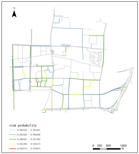
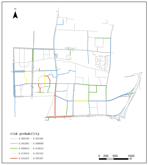
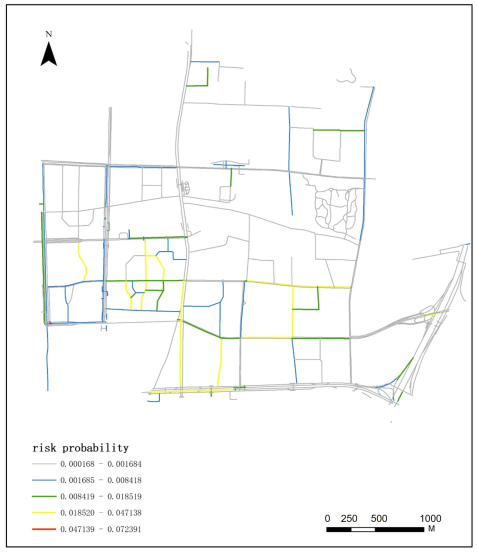
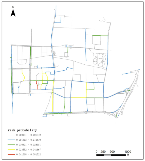
Appendix A. Temporal Variations of Incident Risk

Appendix A.1. Spatial–Temporal Distribution of 110 Incident Risk at 16:00

Applsci 15 03651 i001

Appendix A.2. Spatial–Temporal Distribution of 110 Incident Risk at 17:00

Applsci 15 03651 i002

Appendix A.3. Spatial–Temporal Distribution of 110 Incident Risk at 18:00

Applsci 15 03651 i003

Appendix A.4. Spatial–Temporal Distribution of 110 Incident Risk at 19:00

Applsci 15 03651 i004

Appendix A.5. Spatial–Temporal Distribution of 110 Incident Risk at 20:00

Applsci 15 03651 i005

Appendix A.6. Spatial–Temporal Distribution of 110 Incident Risk at 21:00

Applsci 15 03651 i006

Appendix A.7. Spatial–Temporal Distribution of 110 Incident Risk at 22:00

Applsci 15 03651 i007

Appendix A.8. Spatial–Temporal Distribution of 110 Incident Risk at 23:00

Applsci 15 03651 i008

Appendix B. Simulation Results

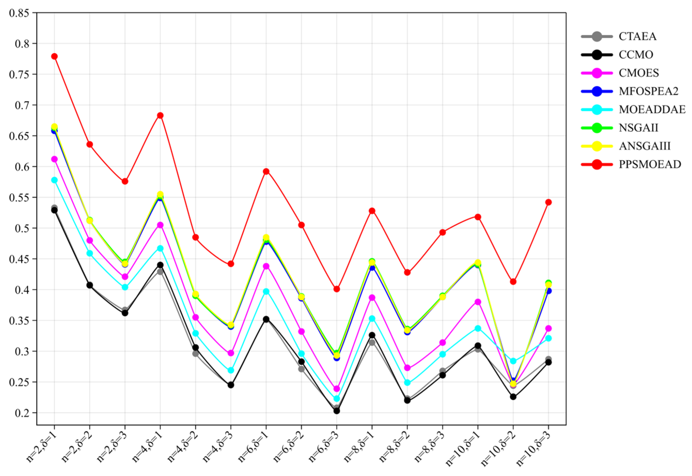
Appendix B.1. Simulation Results of HVs

ScenarioCTAEACCMOCMOESMFOSPEA2MOEADDAENSGAIIANSGAIIIPPSMOEAD
n = 2, δ = 15.3348 × 10⁻¹ (3.13 × 10⁻³)5.2857 × 10⁻¹ (2.16 × 10⁻²)6.1166 × 10⁻¹ (1.49 × 10⁻²)6.5773 × 10⁻¹ (9.12 × 10⁻³)5.7799 × 10⁻¹ (1.47 × 10⁻²)6.6272 × 10⁻¹ (9.72 × 10⁻³)6.6462 × 10⁻¹ (7.26 × 10⁻³) 7.7935 × 10⁻¹ (4.67 × 10⁻²)
n = 2, δ = 24.0827 × 10⁻¹ (3.85 × 10⁻³)4.0660 × 10⁻¹ (1.42 × 10⁻²)4.8040 × 10⁻¹ (9.87 × 10⁻³)5.1152 × 10⁻¹ (6.44 × 10⁻³)4.5867 × 10⁻¹ (7.81 × 10⁻³)5.1307 × 10⁻¹ (7.58 × 10⁻³)5.1213 × 10⁻¹ (4.29 × 10⁻³) 6.3647 × 10⁻¹ (3.31 × 10⁻²)
n = 2, δ = 33.6728 × 10⁻¹ (2.95 × 10⁻³)3.6240 × 10⁻¹ (1.02 × 10⁻²)4.2126 × 10⁻¹ (7.35 × 10⁻³)4.4073 × 10⁻¹ (4.63 × 10⁻³)4.0363 × 10⁻¹ (7.16 × 10⁻³)4.4485 × 10⁻¹ (5.54 × 10⁻³)4.4239 × 10⁻¹ (4.93 × 10⁻³) 5.7622 × 10⁻¹ (4.13 × 10⁻²)
n = 4, δ = 14.2870 × 10⁻¹ (4.60 × 10⁻³)4.3964 × 10⁻¹ (1.85 × 10⁻²)5.0468 × 10⁻¹ (1.33 × 10⁻²)5.4931 × 10⁻¹ (9.64 × 10⁻³)4.6681 × 10⁻¹ (1.22 × 10⁻²)5.5185 × 10⁻¹ (1.01 × 10⁻²)5.5515 × 10⁻¹ (8.91 × 10⁻³) 6.8301 × 10⁻¹ (3.62 × 10⁻²)
n = 4, δ = 22.9579 × 10⁻¹ (2.69 × 10⁻³)3.0601 × 10⁻¹ (1.51 × 10⁻²)3.5539 × 10⁻¹ (7.37 × 10⁻³)3.9056 × 10⁻¹ (6.55 × 10⁻³)3.2916 × 10⁻¹ (6.29 × 10⁻³)3.9047 × 10⁻¹ (7.10 × 10⁻³)3.9262 × 10⁻¹ (5.05 × 10⁻³) 4.8496 × 10⁻¹ (3.51 × 10⁻²)
n = 4, δ = 32.4611 × 10⁻¹ (2.48 × 10⁻³)2.4537 × 10⁻¹ (1.05 × 10⁻²)2.9719 × 10⁻¹ (9.64 × 10⁻³)3.3987 × 10⁻¹ (1.19 × 10⁻²)2.6864 × 10⁻¹ (6.42 × 10⁻³)3.4220 × 10⁻¹ (1.13 × 10⁻²)3.4274 × 10⁻¹ (5.81 × 10⁻³) 4.4168 × 10⁻¹ (3.06 × 10⁻²)
n = 6, δ = 13.5132 × 10⁻¹ (4.68 × 10⁻³)3.5204 × 10⁻¹ (3.08 × 10⁻²)4.3786 × 10⁻¹ (8.90 × 10⁻³)4.7803 × 10⁻¹ (1.18 × 10⁻²)3.9703 × 10⁻¹ (8.56 × 10⁻³)4.8144 × 10⁻¹ (1.41 × 10⁻²)4.8459 × 10⁻¹ (9.71 × 10⁻³) 5.9185 × 10⁻¹ (4.63 × 10⁻²)
n = 6, δ = 22.7068 × 10⁻¹ (3.67 × 10⁻³)2.8270 × 10⁻¹ (1.79 × 10⁻²)3.3246 × 10⁻¹ (9.77 × 10⁻³)3.8599 × 10⁻¹ (7.26 × 10⁻³)2.9647 × 10⁻¹ (7.74 × 10⁻³)3.8864 × 10⁻¹ (8.24 × 10⁻³)3.8777 × 10⁻¹ (6.32 × 10⁻³) 5.0533 × 10⁻¹ (3.73 × 10⁻²)
n = 6, δ = 32.0817 × 10⁻¹ (3.11 × 10⁻³)2.0326 × 10⁻¹ (1.53 × 10⁻²)2.3883 × 10⁻¹ (1.44 × 10⁻²)2.8852 × 10⁻¹ (4.55 × 10⁻³)2.2332 × 10⁻¹ (1.10 × 10⁻²)2.9690 × 10⁻¹ (5.77 × 10⁻³)2.9288 × 10⁻¹ (5.24 × 10⁻³) 4.0057 × 10⁻¹ (3.59 × 10⁻²)
n = 8, δ = 13.1359 × 10⁻¹ (4.02 × 10⁻³)3.2640 × 10⁻¹ (1.97 × 10⁻²)3.8671 × 10⁻¹ (8.16 × 10⁻³)4.3602 × 10⁻¹ (6.67 × 10⁻³)3.5260 × 10⁻¹ (7.02 × 10⁻³)4.4603 × 10⁻¹ (1.23 × 10⁻²)4.4436 × 10⁻¹ (9.44 × 10⁻³) 5.2777 × 10⁻¹ (3.48 × 10⁻²)
n = 8, δ = 22.2254 × 10⁻¹ (2.39 × 10⁻³)2.2038 × 10⁻¹ (1.80 × 10⁻²)2.7292 × 10⁻¹ (7.58 × 10⁻³)3.3128 × 10⁻¹ (6.34 × 10⁻³)2.4899 × 10⁻¹ (6.33 × 10⁻³)3.3554 × 10⁻¹ (7.15 × 10⁻³)3.3391 × 10⁻¹ (6.39 × 10⁻³) 4.2829 × 10⁻¹ (2.87 × 10⁻²)
n = 8, δ = 32.6826 × 10⁻¹ (2.67 × 10⁻³)2.6109 × 10⁻¹ (1.45 × 10⁻²)3.1354 × 10⁻¹ (1.29 × 10⁻²)3.8758 × 10⁻¹ (6.59 × 10⁻³)2.9511 × 10⁻¹ (6.62 × 10⁻³)3.8964 × 10⁻¹ (8.84 × 10⁻³)3.8803 × 10⁻¹ (8.53 × 10⁻³) 4.9269 × 10⁻¹ (4.27 × 10⁻²)
n = 10, δ = 13.0287 × 10⁻¹ (2.85 × 10⁻³)3.0894 × 10⁻¹ (1.87 × 10⁻²)3.7972 × 10⁻¹ (1.31 × 10⁻²)4.4016 × 10⁻¹ (9.30 × 10⁻³)3.3668 × 10⁻¹ (7.51 × 10⁻³)4.4097 × 10⁻¹ (1.02 × 10⁻²)4.4418 × 10⁻¹ (1.13 × 10⁻²) 5.1766 × 10⁻¹ (4.09 × 10⁻²)
n = 10, δ = 22.4442 × 10⁻¹ (3.04 × 10⁻³)2.2647 × 10⁻¹ (1.83 × 10⁻²)2.4613 × 10⁻¹ (3.15 × 10⁻²)2.5201 × 10⁻¹ (5.41 × 10⁻³)2.8382 × 10⁻¹ (4.97 × 10⁻³)2.4699 × 10⁻¹ (5.88 × 10⁻³)2.4722 × 10⁻¹ (4.64 × 10⁻³) 4.1269 × 10⁻¹ (3.02 × 10⁻²)
n = 10, δ = 32.8740 × 10⁻¹ (2.46 × 10⁻³)2.8164 × 10⁻¹ (2.16 × 10⁻²)3.3663 × 10⁻¹ (1.16 × 10⁻²)3.9801 × 10⁻¹ (5.60 × 10⁻³)3.2058 × 10⁻¹ (9.19 × 10⁻³)4.1145 × 10⁻¹ (8.09 × 10⁻³)4.0758 × 10⁻¹ (6.19 × 10⁻³) 5.4163 × 10⁻¹ (5.13 × 10⁻²)
+/−/=0/15/00/15/00/15/00/15/00/15/00/15/00/15/0

Appendix B.2. Simulation Results of Spacings

ScenarioCTAEACCMOCMOESMFOSPEA2MOEADDAENSGAIIANSGAIIIPPSMOEAD
n = 2, δ = 16.5818 × 10⁻³ (9.16 × 10⁻⁴)9.1561 × 10⁻³ (1.11 × 10⁻³)7.4419 × 10⁻³ (1.91 × 10⁻³)8.3420 × 10⁻³ (1.30 × 10⁻³)1.3628 × 10⁻² (4.43 × 10⁻³)8.0466 × 10⁻³ (1.31 × 10⁻³)7.8801 × 10⁻³ (1.10 × 10⁻³)5.9009 × 10⁻³ (1.96 × 10⁻³)
n = 2, δ = 27.2718 × 10⁻³ (9.97 × 10⁻⁴)8.4616 × 10⁻³ (7.43 × 10⁻⁴)8.0992 × 10⁻³ (4.21 × 10⁻³)8.7339 × 10⁻³ (1.39 × 10⁻³)1.5838 × 10⁻² (4.92 × 10⁻³)9.2630 × 10⁻³ (1.24 × 10⁻³)8.6895 × 10⁻³ (1.19 × 10⁻³)6.5355 × 10⁻³ (1.85 × 10⁻³)
n = 2, δ = 37.9941 × 10⁻³ (1.29 × 10⁻³)5.7245 × 10⁻³ (6.22 × 10⁻⁴)7.9817 × 10⁻³ (1.58 × 10⁻³)8.6194 × 10⁻³ (1.17 × 10⁻³)1.6438 × 10⁻² (9.65 × 10⁻³)8.6248 × 10⁻³ (1.40 × 10⁻³)9.0894 × 10⁻³ (1.24 × 10⁻³)7.3637 × 10⁻³ (1.82 × 10⁻³)
n = 4, δ = 17.3373 × 10⁻³ (9.41 × 10⁻⁴)9.4965 × 10⁻³ (1.18 × 10⁻³)8.8465 × 10⁻³ (1.01 × 10⁻³)1.0318 × 10⁻² (1.18 × 10⁻³)1.5295 × 10⁻² (7.18 × 10⁻³)1.0004 × 10⁻² (1.81 × 10⁻³)9.1592 × 10⁻³ (1.29 × 10⁻³)7.1025 × 10⁻³ (1.86 × 10⁻³)
n = 4, δ = 28.2588 × 10⁻³ (1.13 × 10⁻³)8.3543 × 10⁻³ (1.36 × 10⁻³)9.9683 × 10⁻³ (2.04 × 10⁻³)1.0789 × 10⁻² (1.28 × 10⁻³)1.4847 × 10⁻² (4.47 × 10⁻³)1.0888 × 10⁻² (1.41 × 10⁻³)1.0950 × 10⁻² (1.68 × 10⁻³)9.2828 × 10⁻³ (3.54 × 10⁻³)
n = 4, δ = 38.0457 × 10⁻³ (1.45 × 10⁻³)1.0590 × 10⁻² (1.41 × 10⁻³)9.2606 × 10⁻³ (1.82 × 10⁻³)1.0944 × 10⁻² (1.88 × 10⁻³)1.4683 × 10⁻² (4.24 × 10⁻³)1.0411 × 10⁻² (1.56 × 10⁻³)1.0757 × 10⁻² (1.48 × 10⁻³)8.6537 × 10⁻³ (6.87 × 10⁻³)
n = 6, δ = 11.0195 × 10⁻² (1.08 × 10⁻³)7.3334 × 10⁻³ (7.89 × 10⁻⁴)1.0349 × 10⁻² (5.07 × 10⁻³)1.3157 × 10⁻² (2.19 × 10⁻³)1.9295 × 10⁻² (6.11 × 10⁻³)1.2003 × 10⁻² (2.07 × 10⁻³)1.2825 × 10⁻² (2.09 × 10⁻³)7.9827 × 10⁻³ (3.27 × 10⁻³)
n = 6, δ = 28.7095 × 10⁻³ (1.09 × 10⁻³)1.0669 × 10⁻² (1.41 × 10⁻³)9.5790 × 10⁻³ (3.45 × 10⁻⁴)1.1537 × 10⁻² (1.69 × 10⁻³)1.5809 × 10⁻² (4.70 × 10⁻³)1.1008 × 10⁻² (1.74 × 10⁻³)1.1550 × 10⁻² (1.60 × 10⁻³)6.7823 × 10⁻³ (3.01 × 10⁻³)
n = 6, δ = 31.0716 × 10⁻² (2.37 × 10⁻³)6.6066 × 10⁻³ (3.39 × 10⁻³)8.4693 × 10⁻³ (3.01 × 10⁻³)1.0556 × 10⁻² (1.45 × 10⁻³)1.4818 × 10⁻² (6.36 × 10⁻³)1.0304 × 10⁻² (1.55 × 10⁻³)1.0034 × 10⁻² (1.54 × 10⁻³)4.7195 × 10⁻³ (2.83 × 10⁻³)
n = 8, δ = 11.0063 × 10⁻² (1.33 × 10⁻³)9.6572 × 10⁻³ (9.84 × 10⁻⁴)1.0377 × 10⁻² (5.84 × 10⁻⁴)1.2151 × 10⁻² (1.56 × 10⁻³)1.6886 × 10⁻² (5.38 × 10⁻³)1.2111 × 10⁻² (1.87 × 10⁻³)1.2705 × 10⁻² (1.60 × 10⁻³)8.4812 × 10⁻³ (3.45 × 10⁻³)
n = 8, δ = 29.5034 × 10⁻³ (1.90 × 10⁻³)1.2068 × 10⁻³ (3.14 × 10⁻³)8.5870 × 10⁻³ (1.81 × 10⁻³)1.1927 × 10⁻² (1.54 × 10⁻³)1.5408 × 10⁻² (4.34 × 10⁻³)1.1699 × 10⁻² (1.47 × 10⁻³)1.2034 × 10⁻² (2.43 × 10⁻³)6.9181 × 10⁻³ (6.03 × 10⁻³)
n = 8, δ = 38.7741 × 10⁻³ (1.35 × 10⁻³)6.8553 × 10⁻⁴ (2.78 × 10⁻³)8.1039 × 10⁻³ (1.54 × 10⁻³)1.1620 × 10⁻² (1.93 × 10⁻³)1.4346 × 10⁻² (4.99 × 10⁻³)1.1752 × 10⁻² (1.90 × 10⁻³)1.1614 × 10⁻² (1.57 × 10⁻³)6.0393 × 10⁻³ (5.08 × 10⁻³)
n = 10, δ = 19.2486 × 10⁻³ (1.16 × 10⁻³)1.1389 × 10⁻² (1.54 × 10⁻³)1.0777 × 10⁻² (1.45 × 10⁻³)1.2465 × 10⁻² (1.99 × 10⁻³)1.5472 × 10⁻² (3.69 × 10⁻³)1.2154 × 10⁻² (2.01 × 10⁻³)1.2186 × 10⁻² (2.17 × 10⁻³)9.9395 × 10⁻³ (5.08 × 10⁻³)
n = 10, δ = 21.0917 × 10⁻² (1.82 × 10⁻³)6.1531 × 10⁻³ (3.26 × 10⁻³)8.5457 × 10⁻³ (2.36 × 10⁻³)1.1245 × 10⁻² (1.35 × 10⁻³)1.5906 × 10⁻² (4.62 × 10⁻³)9.9491 × 10⁻³ (9.71 × 10⁻⁴)1.0682 × 10⁻² (1.23 × 10⁻³)3.5137 × 10⁻³ (1.74 × 10⁻³)
n = 10, δ = 38.4370 × 10⁻³ (1.15 × 10⁻³)2.9216 × 10⁻⁴ (1.04 × 10⁻³)7.4574 × 10⁻³ (1.89 × 10⁻³)1.0371 × 10⁻² (1.41 × 10⁻³)1.3705 × 10⁻² (3.80 × 10⁻³)1.0791 × 10⁻² (1.74 × 10⁻³)1.1029 × 10⁻² (1.57 × 10⁻³)5.0337 × 10⁻³ (5.02 × 10⁻³)
+/−/=3/12/04/11/00/15/00/15/00/15/00/15/00/15/0

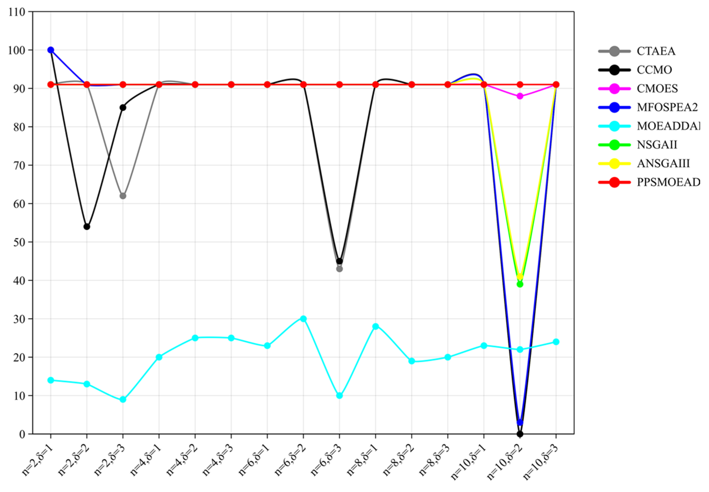
Appendix B.3. Simulation Results of Feasible Solutions

ScenarioCTAEACCMOCMOESMFOSPEA2MOEADDAENSGAIIANSGAIIIPPSMOEAD
n = 2, δ = 19.1000 × 101 (0.00 × 100) 1.0000 × 10² (0.00 × 100) 1.0000 × 10² (0.00 × 100) 1.0000 × 10² (0.00 × 100) 1.4000 × 101 (2.00 × 100) 9.1000 × 101 (0.00 × 100) 9.1000 × 101 (0.00 × 100) 9.1000 × 101 (0.00 × 100)
n = 2, δ = 29.1000 × 101 (0.00 × 100) 5.4667 × 101 (2.47 × 101) 9.1000 × 101 (0.00 × 100) 9.1000 × 101 (0.00 × 100) 1.3667 × 101 (2.08 × 100) 9.1000 × 101 (0.00 × 100) 9.1000 × 101 (0.00 × 100) 9.1000 × 101 (0.00 × 100)
n = 2, δ = 36.2667 × 101 (6.11 × 100) 8.5333 × 101 (6.03 × 100) 9.1000 × 101 (0.00 × 100) 9.1000 × 101 (0.00 × 100) 9.3333 × 100 (3.06 × 100) 9.1000 × 101 (0.00 × 100) 9.1000 × 101 (0.00 × 100) 9.1000 × 101 (0.00 × 100)
n = 4, δ = 19.1000 × 101 (0.00 × 100) 9.1000 × 101 (0.00 × 100) 9.1000 × 101 (0.00 × 100) 9.1000 × 101 (0.00 × 100) 2.0667 × 101 (4.51 × 100) 9.1000 × 101 (0.00 × 100) 9.1000 × 101 (0.00 × 100) 9.1000 × 101 (0.00 × 100)
n = 4, δ = 29.1000 × 101 (0.00 × 100) 9.1000 × 101 (0.00 × 100) 9.1000 × 101 (0.00 × 100) 9.1000 × 101 (0.00 × 100) 2.5000 × 101 (2.00 × 100) 9.1000 × 101 (0.00 × 100) 9.1000 × 101 (0.00 × 100) 9.1000 × 101 (0.00 × 100)
n = 4, δ = 39.1000 × 101 (0.00 × 100) 9.1000 × 101 (0.00 × 100) 9.1000 × 101 (0.00 × 100) 9.1000 × 101 (0.00 × 100) 2.5000 × 101 (4.36 × 100) 9.1000 × 101 (0.00 × 100) 9.1000 × 101 (0.00 × 100) 9.1000 × 101 (0.00 × 100)
n = 6, δ = 19.1000 × 101 (0.00 × 100) 9.1000 × 101 (0.00 × 100) 9.1000 × 101 (0.00 × 100) 9.1000 × 101 (0.00 × 100) 2.3000 × 101 (2.00 × 100) 9.1000 × 101 (0.00 × 100) 9.1000 × 101 (0.00 × 100) 9.1000 × 101 (0.00 × 100)
n = 6, δ = 29.1000 × 101 (0.00 × 100) 9.1000 × 101 (0.00 × 100) 9.1000 × 101 (0.00 × 100) 9.1000 × 101 (0.00 × 100) 3.0333 × 101 (5.03 × 100) 9.1000 × 101 (0.00 × 100) 9.1000 × 101 (0.00 × 100) 9.1000 × 101 (0.00 × 100)
n = 6, δ = 34.3333 × 101 (7.57 × 100) 4.5000 × 101 (4.50 × 101) 9.1000 × 101 (0.00 × 100) 9.1000 × 101 (0.00 × 100) 1.0333 × 101 (5.77 × 10⁻¹) 9.1000 × 101 (0.00 × 100) 9.1000 × 101 (0.00 × 100) 9.1000 × 101 (0.00 × 100)
n = 8, δ = 19.1000 × 101 (0.00 × 100) 9.1000 × 101 (0.00 × 100) 9.1000 × 101 (0.00 × 100) 9.1000 × 101 (0.00 × 100) 2.8333 × 101 (1.15 × 100) 9.1000 × 101 (0.00 × 100) 9.1000 × 101 (0.00 × 100) 9.1000 × 101 (0.00 × 100)
n = 8, δ = 29.1000 × 101 (0.00 × 100) 9.1000 × 101 (0.00 × 100) 9.1000 × 101 (0.00 × 100) 9.1000 × 101 (0.00 × 100) 1.9000 × 101 (5.57 × 100) 9.1000 × 101 (0.00 × 100) 9.1000 × 101 (0.00 × 100) 9.1000 × 101 (0.00 × 100)
n = 8, δ = 39.1000 × 101 (0.00 × 100) 9.1000 × 101 (0.00 × 100) 9.1000 × 101 (0.00 × 100) 9.1000 × 101 (0.00 × 100) 2.0333 × 101 (9.45 × 100) 9.1000 × 101 (0.00 × 100) 9.1000 × 101 (0.00 × 100) 9.1000 × 101 (0.00 × 100)
n = 10, δ = 19.1000 × 101 (0.00 × 100) 9.1000 × 101 (0.00 × 100) 9.1000 × 101 (0.00 × 100) 9.1000 × 101 (0.00 × 100) 2.3333 × 101 (9.02 × 100) 9.1000 × 101 (0.00 × 100) 9.1000 × 101 (0.00 × 100) 9.1000 × 101 (0.00 × 100)
n = 10, δ = 20.0000 × 100 (0.00 × 100) 0.0000 × 100 (0.00 × 100) 8.8000 × 101 (0.00 × 100) 3.3333 × 100 (3.21 × 100) 2.2667 × 101 (1.02 × 101) 3.9000 × 101 (9.54 × 100) 4.1667 × 101 (1.29 × 101) 9.1000 × 101 (0.00 × 100)
n = 10, δ = 39.1000 × 101 (0.00 × 100) 9.1000 × 101 (0.00 × 100) 9.1000 × 101 (0.00 × 100) 9.1000 × 101 (0.00 × 100) 2.4000 × 101 (7.81 × 100) 9.1000 × 101 (0.00 × 100) 9.1000 × 101 (0.00 × 100) 9.1000 × 101 (0.00 × 100)
+/−/=0/3/121/4/101/0/141/1/130/15/00/1/140/1/14

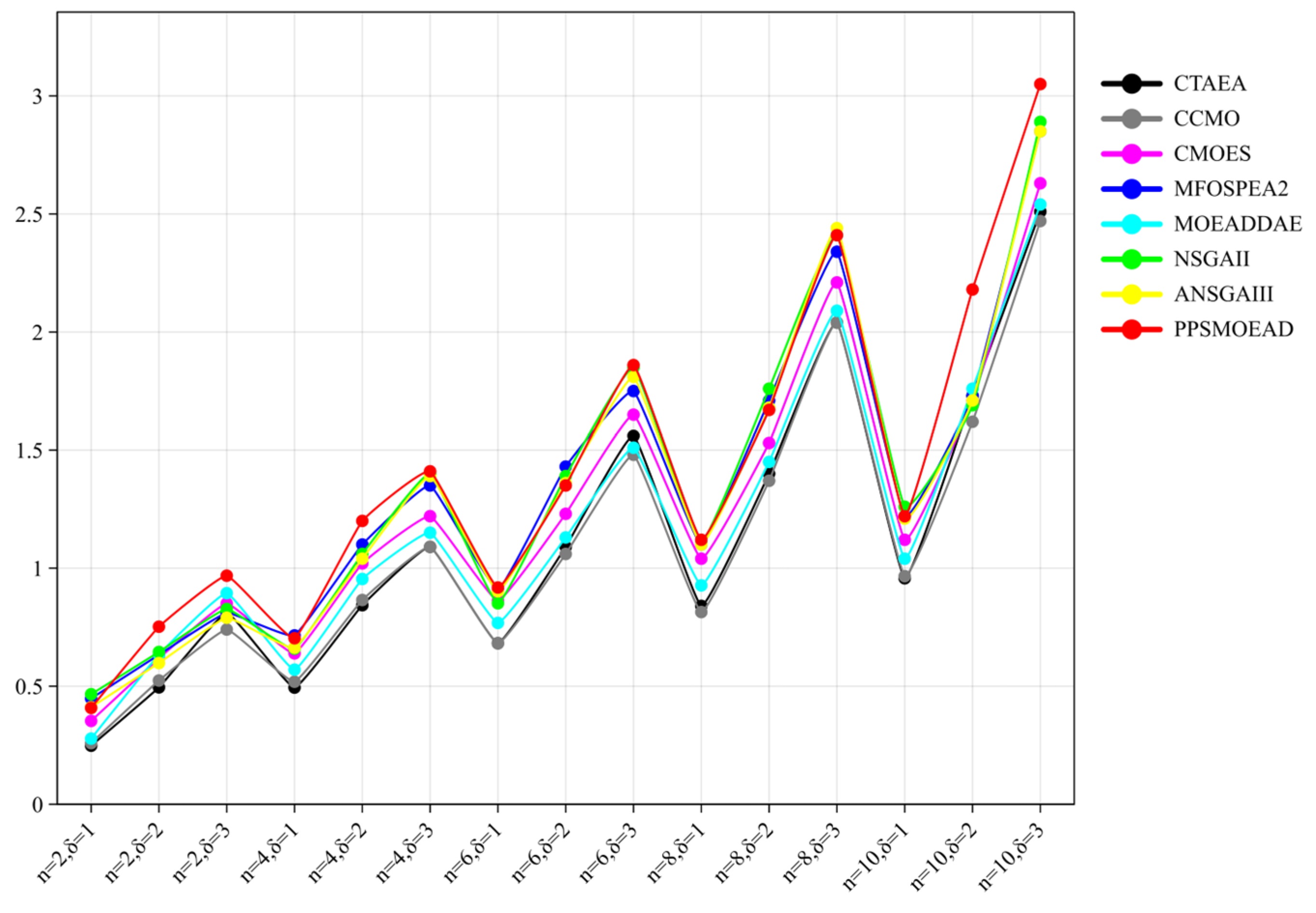
Appendix B.4. Simulation Results of Objective 1

ScenarioCTAEACCMOCMOESMFOSPEA2MOEADDAENSGAIIANSGAIIIPPSMOEAD
n = 2, δ = 12.4817 × 10⁻¹ (1.26 × 10⁻³) 2.5932 × 10⁻¹ (2.80 × 10⁻²) 3.5309 × 10⁻¹ (2.11 × 10⁻²) 4.4772 × 10⁻¹ (1.38 × 10⁻²) 2.7817 × 10⁻¹ (1.36 × 10⁻²) 4.6625 × 10⁻¹ (2.95 × 10⁻³) 4.1123 × 10⁻¹ (2.23 × 10⁻²) 4.0792 × 10⁻¹ (1.35 × 10⁻²)
n = 2, δ = 24.9522 × 10⁻¹ (7.51 × 10⁻³) 5.2383 × 10⁻¹ (4.65 × 10⁻²) 6.1791 × 10⁻¹ (1.97 × 10⁻²) 6.3325 × 10⁻¹ (3.61 × 10⁻²) 6.3355 × 10⁻¹ (4.63 × 10⁻²) 6.4490 × 10⁻¹ (5.99 × 10⁻²) 5.9804 × 10⁻¹ (2.00 × 10⁻²) 7.5154 × 10⁻¹ (3.08 × 10⁻²)
n = 2, δ = 38.1012 × 10⁻¹ (1.09 × 10⁻²) 7.3987 × 10⁻¹ (2.89 × 10⁻²) 8.5003 × 10⁻¹ (5.24 × 10⁻²) 8.0960 × 10⁻¹ (3.45 × 10⁻²) 8.9352 × 10⁻¹ (6.85 × 10⁻²) 8.2722 × 10⁻¹ (6.11 × 10⁻²) 7.8969 × 10⁻¹ (2.66 × 10⁻²) 9.6774 × 10⁻¹ (4.99 × 10⁻²)
n = 4, δ = 14.9363 × 10⁻¹ (1.02 × 10⁻²) 5.1893 × 10⁻¹ (2.88 × 10⁻²) 6.3893 × 10⁻¹ (2.31 × 10⁻²) 7.1475 × 10⁻¹ (2.26 × 10⁻²) 5.6962 × 10⁻¹ (1.14 × 10⁻²) 6.5933 × 10⁻¹ (1.50 × 10⁻²) 6.6272 × 10⁻¹ (3.23 × 10⁻²) 7.0257 × 10⁻¹ (4.98 × 10⁻²)
n = 4, δ = 28.4295 × 10⁻¹ (9.26 × 10⁻³) 8.6454 × 10⁻¹ (6.74 × 10⁻³) 1.0166 × 100 (4.99 × 10⁻²) 1.1016 × 100 (1.94 × 10⁻²) 9.5372 × 10⁻¹ (3.20 × 10⁻²) 1.0595 × 100 (3.27 × 10⁻²) 1.0399 × 100 (7.74 × 10⁻²) 1.1984 × 100 (2.46 × 10⁻²)
n = 4, δ = 31.0945 × 100 (7.57 × 10⁻³) 1.0927 × 100 (3.74 × 10⁻²) 1.2188 × 100 (4.19 × 10⁻²) 1.3479 × 100 (4.20 × 10⁻²) 1.1461 × 100 (9.38 × 10⁻³) 1.4049 × 100 (2.75 × 10⁻²) 1.3939 × 100 (2.17 × 10⁻²) 1.4071 × 100 (1.01 × 10⁻¹)
n = 6, δ = 16.8233 × 10⁻¹ (1.33 × 10⁻²) 6.8118 × 10⁻¹ (6.17 × 10⁻²) 8.6174 × 10⁻¹ (7.72 × 10⁻²) 9.0913 × 10⁻¹ (1.68 × 10⁻²) 7.6764 × 10⁻¹ (3.87 × 10⁻²) 8.5093 × 10⁻¹ (3.84 × 10⁻²) 9.0246 × 10⁻¹ (1.68 × 10⁻²) 9.1786 × 10⁻¹ (3.19 × 10⁻²)
n = 6, δ = 21.0891 × 100 (2.92 × 10⁻³) 1.0615 × 100 (8.06 × 10⁻²) 1.2306 × 100 (1.84 × 10⁻²) 1.4326 × 100 (4.79 × 10⁻²) 1.1270 × 100 (4.09 × 10⁻⁴) 1.3935 × 100 (3.21 × 10⁻²) 1.3630 × 100 (3.05 × 10⁻²) 1.3539 × 100 (5.37 × 10⁻²)
n = 6, δ = 31.5612 × 100 (2.76 × 10⁻²) 1.4803 × 100 (4.44 × 10⁻²) 1.6517 × 100 (4.96 × 10⁻²) 1.7485 × 100 (2.44 × 10⁻²) 1.5143 × 100 (7.32 × 10⁻³) 1.8495 × 100 (3.39 × 10⁻²) 1.8136 × 100 (8.47 × 10⁻³) 1.8570 × 100 (7.76 × 10⁻²)
n = 8, δ = 18.3965 × 10⁻¹ (3.23 × 10⁻³) 8.1370 × 10⁻¹ (4.94 × 10⁻²) 1.0404 × 100 (4.57 × 10⁻²) 1.0991 × 100 (2.11 × 10⁻²) 9.2728 × 10⁻¹ (2.23 × 10⁻²) 1.1058 × 100 (6.77 × 10⁻²) 1.1006 × 100 (5.41 × 10⁻²) 1.1188 × 100 (7.55 × 10⁻²)
n = 8, δ = 21.3957 × 100 (3.41 × 10⁻³) 1.3735 × 100 (1.61 × 10⁻²) 1.5348 × 100 (4.47 × 10⁻²) 1.7119 × 100 (3.28 × 10⁻²) 1.4531 × 100 (1.36 × 10⁻²) 1.7565 × 100 (8.31 × 10⁻³) 1.6848 × 100 (1.73 × 10⁻²) 1.6690 × 100 (6.62 × 10⁻²)
n = 8, δ = 32.0392 × 100 (1.56 × 10⁻²) 2.0418 × 100 (5.52 × 10⁻²) 2.2068 × 100 (3.41 × 10⁻²) 2.3407 × 100 (5.11 × 10⁻²) 2.0882 × 100 (2.17 × 10⁻²) 2.4116 × 100 (4.70 × 10⁻²) 2.4392 × 100 (3.89 × 10⁻²) 2.4071 × 100 (6.05 × 10⁻²)
n = 10, δ = 19.5739 × 10⁻¹ (3.22 × 10⁻³) 9.6618 × 10⁻¹ (1.64 × 10⁻²) 1.1217 × 100 (2.03 × 10⁻²) 1.2225 × 100 (6.11 × 10⁻²) 1.0409 × 100 (2.69 × 10⁻³) 1.2584 × 100 (1.48 × 10⁻²) 1.2097 × 100 (3.61 × 10⁻²) 1.2242 × 100 (2.65 × 10⁻²)
n = 10, δ = 21.7291 × 100 (9.14 × 10⁻³) 1.6209 × 100 (1.57 × 10⁻²) 1.7113 × 100 (1.48 × 10⁻¹) 1.7272 × 100 (1.57 × 10⁻²) 1.7584 × 100 (2.94 × 10⁻²) 1.6935 × 100 (8.17 × 10⁻³) 1.7085 × 100 (2.41 × 10⁻²) 2.1771 × 100 (1.24 × 10⁻¹)
n = 10, δ = 32.5061 × 100 (5.22 × 10⁻³) 2.4677 × 100 (2.68 × 10⁻²) 2.6333 × 100 (3.19 × 10⁻²) 2.8504 × 100 (6.03 × 10⁻²) 2.5354 × 100 (2.12 × 10⁻²) 2.8915 × 100 (4.65 × 10⁻²) 2.8543 × 100 (5.37 × 10⁻²) 3.0549 × 100 (1.62 × 10⁻¹)
+/−/=0/15/00/15/00/15/04/11/00/15/05/10/04/11/0

Appendix B.5. Simulation Results of Objective 2

InstanceCTAEACCMOCMOESMFOSPEA2MOEADDAENSGAIIANSGAIIIPPSMOEAD
n = 2, δ = 11.7727 × 10⁴ (1.43 × 10²) 1.8022 × 10⁴ (1.29 × 10²) 2.0588 × 10⁴ (1.14 × 10³) 2.4076 × 10⁴ (7.37 × 10²) 1.9263 × 10⁴ (3.74 × 10²) 2.4688 × 10⁴ (8.85 × 10²) 2.4127 × 10⁴ (6.38 × 10²) 2.0638 × 10⁴ (4.69 × 10²)
n = 2, δ = 23.3822 × 10⁴ (4.64 × 10²) 3.2241 × 10⁴ (2.04 × 10²) 3.8145 × 10⁴ (1.20 × 10³) 4.1432 × 10⁴ (4.83 × 10²) 3.5377 × 10⁴ (4.04 × 10²) 4.1059 × 10⁴ (4.47 × 10²) 4.1152 × 10⁴ (1.35 × 10³) 3.9393 × 10⁴ (5.58 × 10²)
n = 2, δ = 35.0284 × 10⁴ (2.44 × 10²) 4.9192 × 10⁴ (1.22 × 10³) 5.4440 × 10⁴ (1.76 × 10³) 5.7983 × 10⁴ (3.70 × 10²) 5.2263 × 10⁴ (9.42 × 10²) 5.7121 × 10⁴ (7.92 × 10²) 5.6060 × 10⁴ (1.06 × 10³) 5.9698 × 10⁴ (1.09 × 10³)
n = 4, δ = 13.5272 × 10⁴ (3.62 × 10²) 3.4690 × 10⁴ (1.26 × 10³) 3.9287 × 10⁴ (1.12 × 10³) 4.3048 × 10⁴ (7.46 × 10²) 3.7738 × 10⁴ (4.72 × 10²) 4.3508 × 10⁴ (1.02 × 10³) 4.2714 × 10⁴ (7.26 × 10²) 4.2682 × 10⁴ (3.58 × 10³)
n = 4, δ = 26.7110 × 10⁴ (7.83 × 101) 6.8976 × 10⁴ (7.57 × 10²) 7.2056 × 10⁴ (1.79 × 10³) 7.5904 × 10⁴ (1.43 × 10³) 6.9781 × 10⁴ (6.86 × 10²) 7.7915 × 10⁴ (1.19 × 10³) 7.7411 × 10⁴ (2.13 × 10³) 7.6844 × 10⁴ (2.12 × 10³)
n = 4, δ = 39.7741 × 10⁴ (3.84 × 10²) 9.8781 × 10⁴ (1.80 × 10³) 1.0692 × 10⁵ (4.98 × 10³) 1.1029 × 10⁵ (1.80 × 10³) 1.0005 × 10⁵ (1.51 × 10³) 1.1123 × 10⁵ (5.02 × 10²) 1.0932 × 10⁵ (1.06 × 10³) 1.1187 × 10⁵ (2.09 × 10³)
n = 6, δ = 15.1724 × 10⁴ (3.05 × 10²) 5.4440 × 10⁴ (7.61 × 10²) 5.5556 × 10⁴ (1.19 × 10³) 6.1670 × 10⁴ (1.08 × 10³) 5.5295 × 10⁴ (8.51 × 10²) 6.4550 × 10⁴ (1.64 × 10³) 6.2320 × 10⁴ (1.33 × 10³) 5.8331 × 10⁴ (1.87 × 10³)
n = 6, δ = 29.8313 × 10⁴ (2.09 × 10²) 9.7560 × 10⁴ (4.14 × 10³) 1.0449 × 10⁵ (2.08 × 10³) 1.1013 × 10⁵ (1.05 × 10³) 1.0053 × 10⁵ (1.06 × 10³) 1.1247 × 10⁵ (7.75 × 10²) 1.1230 × 10⁵ (1.85 × 10³) 1.1595 × 10⁵ (6.06 × 10³)
n = 6, δ = 31.3832 × 10⁵ (2.01 × 10²) 1.4163 × 10⁵ (3.69 × 10³) 1.4660 × 10⁵ (2.91 × 10³) 1.5496 × 10⁵ (1.09 × 10³) 1.4202 × 10⁵ (1.94 × 10³) 1.5588 × 10⁵ (9.57 × 10²) 1.5359 × 10⁵ (7.29 × 10²) 1.7371 × 10⁵ (8.88 × 10³)
n = 8, δ = 16.7441 × 10⁴ (2.78 × 10²) 6.9070 × 10⁴ (3.49 × 10³) 7.2571 × 10⁴ (1.81 × 10³) 7.8538 × 10⁴ (2.45 × 10³) 7.0495 × 10⁴ (1.22 × 10²) 7.7522 × 10⁴ (1.47 × 10³) 8.0767 × 10⁴ (5.68 × 10²) 7.6902 × 10⁴ (2.69 × 10³)
n = 8, δ = 21.2778 × 10⁵ (6.84 × 101) 1.2569 × 10⁵ (3.65 × 10³) 1.3437 × 10⁵ (1.58 × 10³) 1.4098 × 10⁵ (2.48 × 10³) 1.3207 × 10⁵ (1.42 × 10³) 1.4308 × 10⁵ (2.19 × 10³) 1.4060 × 10⁵ (1.84 × 10³) 1.4925 × 10⁵ (2.05 × 10³)
n = 8, δ = 31.9028 × 10⁵ (4.46 × 10²) 1.9089 × 10⁵ (6.08 × 10³) 1.9299 × 10⁵ (1.70 × 10³) 2.0709 × 10⁵ (1.85 × 10³) 1.9274 × 10⁵ (1.08 × 10³) 2.0701 × 10⁵ (1.05 × 10³) 2.0459 × 10⁵ (9.39 × 10²) 2.2425 × 10⁵ (1.25 × 10⁴)
n = 10, δ = 18.2917 × 10⁴ (4.49 × 10²) 8.4949 × 10⁴ (1.30 × 10³) 9.0857 × 10⁴ (1.62 × 10³) 9.5876 × 10⁴ (1.57 × 10³) 8.4002 × 10⁴ (1.23 × 10³) 9.4965 × 10⁴ (1.55 × 10³) 9.4282 × 10⁴ (1.15 × 10³) 9.6150 × 10⁴ (2.49 × 10²)
n = 10, δ = 21.5193 × 10⁵ (1.11 × 10³) 1.5152 × 10⁵ (2.67 × 10³) 1.6486 × 10⁵ (8.78 × 10³) 1.5767 × 10⁵ (8.00 × 101) 1.6403 × 10⁵ (2.06 × 10³) 1.5699 × 10⁵ (1.42 × 10³) 1.5711 × 10⁵ (1.12 × 10³) 1.8937 × 10⁵ (2.94 × 10³)
n = 10, δ = 32.3515 × 10⁵ (2.63 × 10²) 2.3337 × 10⁵ (3.53 × 10³) 2.3846 × 10⁵ (3.58 × 10³) 2.5497 × 10⁵ (2.41 × 10³) 2.3726 × 10⁵ (1.26 × 10³) 2.5447 × 10⁵ (4.72 × 10³) 2.5390 × 10⁵ (2.64 × 10³) 2.7748 × 10⁵ (6.40 × 10³)
+/−/=0/15/00/15/00/15/05/10/00/15/06/9/06/9/0

Appendix B.6. Simulation Results of Objective 3

InstanceCTAEACCMOCMOESMFOSPEA2MOEADDAENSGAIIANSGAIIIPPSMOEAD
n = 2, δ = 11.2919 × 10⁵ (1.35 × 10³) 1.2839 × 10⁵ (1.83 × 10²) 1.1826 × 10⁵ (1.88 × 10³) 1.1443 × 10⁵ (1.14 × 10³) 1.2171 × 10⁵ (3.65 × 10³) 1.1372 × 10⁵ (1.40 × 10³) 1.1252 × 10⁵ (1.50 × 10³) 7.5361 × 10⁴ (3.16 × 10³)
n = 2, δ = 22.7239 × 10⁵ (7.65 × 10²) 2.7738 × 10⁵ (2.18 × 10³) 2.5961 × 10⁵ (4.43 × 10³) 2.5567 × 10⁵ (2.20 × 10³) 2.6387 × 10⁵ (2.10 × 10³) 2.5443 × 10⁵ (3.27 × 10³) 2.5230 × 10⁵ (3.25 × 10³) 1.7882 × 10⁵ (1.47 × 10⁴)
n = 2, δ = 34.2055 × 10⁵ (1.64 × 10³) 4.1639 × 10⁵ (4.62 × 10³) 4.0550 × 10⁵ (5.57 × 10²) 3.9671 × 10⁵ (3.09 × 10³) 4.0551 × 10⁵ (6.65 × 10³) 3.9399 × 10⁵ (1.17 × 10³) 3.9379 × 10⁵ (2.43 × 10³) 2.9215 × 10⁵ (8.22 × 10³)
n = 4, δ = 12.4098 × 10⁵ (5.24 × 10²) 2.3753 × 10⁵ (1.33 × 10⁴) 2.2364 × 10⁵ (4.93 × 10³) 2.1782 × 10⁵ (5.31 × 10³) 2.2975 × 10⁵ (3.66 × 10³) 2.1643 × 10⁵ (1.40 × 10³) 2.1552 × 10⁵ (3.82 × 10³) 1.3194 × 10⁵ (8.98 × 10³)
n = 4, δ = 25.0742 × 10⁵ (1.23 × 10³) 4.9994 × 10⁵ (1.37 × 10⁴) 4.7946 × 10⁵ (7.65 × 10³) 4.7885 × 10⁵ (5.40 × 10³) 4.9697 × 10⁵ (5.34 × 10³) 4.7530 × 10⁵ (1.03 × 10³) 4.7989 × 10⁵ (4.16 × 10³) 3.6180 × 10⁵ (1.68 × 10⁴)
n = 4, δ = 37.8411 × 10⁵ (1.61 × 10³) 7.9697 × 10⁵ (2.53 × 10⁴) 7.6126 × 10⁵ (7.16 × 10³) 7.4288 × 10⁵ (5.39 × 10³) 7.6981 × 10⁵ (3.79 × 10³) 7.3724 × 10⁵ (6.99 × 10³) 7.3935 × 10⁵ (4.67 × 10³) 5.3602 × 10⁵ (2.56 × 10⁴)
n = 6, δ = 13.3590 × 10⁵ (7.14 × 10²) 3.3709 × 10⁵ (9.05 × 10³) 3.0870 × 10⁵ (3.12 × 10³) 3.0525 × 10⁵ (2.10 × 10³) 3.2724 × 10⁵ (7.76 × 10³) 3.0529 × 10⁵ (1.08 × 10⁴) 3.0693 × 10⁵ (4.01 × 10³) 1.9522 × 10⁵ (1.65 × 10⁴)
n = 6, δ = 27.1079 × 10⁵ (1.50 × 10³) 7.0456 × 10⁵ (3.20 × 10⁴) 6.8745 × 10⁵ (4.84 × 10³) 6.5767 × 10⁵ (1.95 × 10³) 7.0125 × 10⁵ (5.11 × 10³) 6.5358 × 10⁵ (4.52 × 10³) 6.6843 × 10⁵ (6.47 × 10³) 4.6995 × 10⁵ (4.43 × 10⁴)
n = 6, δ = 31.0855 × 10⁶ (6.48 × 10³) 1.1004 × 10⁶ (1.21 × 10⁴) 1.0632 × 10⁶ (1.14 × 10⁴) 1.0322 × 10⁶ (2.93 × 10³) 1.0780 × 10⁶ (1.19 × 10⁴) 1.0336 × 10⁶ (8.82 × 10³) 1.0345 × 10⁶ (2.37 × 10³) 7.7564 × 10⁵ (2.23 × 10⁴)
n = 8, δ = 14.2071 × 10⁵ (2.30 × 10³) 4.1537 × 10⁵ (8.78 × 10³) 3.9588 × 10⁵ (5.10 × 10³) 3.8614 × 10⁵ (3.55 × 10³) 4.0899 × 10⁵ (1.67 × 10³) 3.8687 × 10⁵ (5.55 × 10³) 3.8388 × 10⁵ (9.64 × 10³) 3.0375 × 10⁵ (2.53 × 10³)
n = 8, δ = 28.8451 × 10⁵ (3.10 × 10³) 8.9239 × 10⁵ (2.28 × 10⁴) 8.5474 × 10⁵ (4.11 × 10³) 8.2790 × 10⁵ (3.08 × 10³) 8.7196 × 10⁵ (7.20 × 10³) 8.3360 × 10⁵ (1.17 × 10⁴) 8.2955 × 10⁵ (1.22 × 10⁴) 6.1058 × 10⁵ (1.69 × 10⁴)
n = 8, δ = 31.3454 × 10⁶ (4.19 × 10³) 1.3274 × 10⁶ (2.14 × 10⁴) 1.3194 × 10⁶ (9.78 × 10³) 1.2680 × 10⁶ (3.76 × 10³) 1.3199 × 10⁶ (2.50 × 10³) 1.2740 × 10⁶ (1.30 × 10⁴) 1.2739 × 10⁶ (5.92 × 10³) 9.7669 × 10⁵ (1.01 × 10⁴)
n = 10, δ = 15.0129 × 10⁵ (1.04 × 10³) 5.0015 × 10⁵ (1.49 × 10⁴) 4.8192 × 10⁵ (4.26 × 10³) 4.5969 × 10⁵ (3.77 × 10³) 4.8550 × 10⁵ (4.63 × 10³) 4.5871 × 10⁵ (5.93 × 10³) 4.6011 × 10⁵ (2.80 × 10³) 3.3833 × 10⁵ (2.41 × 10⁴)
n = 10, δ = 21.0403 × 10⁶ (6.76 × 10³) 1.0609 × 10⁶ (2.78 × 10⁴) 1.0555 × 10⁶ (1.73 × 10⁴) 1.0412 × 10⁶ (5.75 × 10²) 1.0225 × 10⁶ (1.28 × 10⁴) 1.0481 × 10⁶ (8.41 × 10³) 1.0505 × 10⁶ (6.88 × 10³) 7.3307 × 10⁵ (1.06 × 10⁴)
n = 10, δ = 31.5821 × 10⁶ (3.20 × 10³) 1.5879 × 10⁶ (1.90 × 10⁴) 1.5642 × 10⁶ (9.22 × 10³) 1.5147 × 10⁶ (9.67 × 10³) 1.5629 × 10⁶ (1.14 × 10⁴) 1.5031 × 10⁶ (6.47 × 10²) 1.5062 × 10⁶ (7.84 × 10³) 1.1677 × 10⁶ (1.75 × 10⁴)
+/−/=0/15/00/15/00/15/00/15/00/15/00/15/00/15/0

References

  1. Samanta, S.; Sen, G.; Ghosh, S.K. A Literature Review on Police Patrolling Problems. Ann. Oper. Res. 2022, 316, 1063–1106. [Google Scholar] [CrossRef]
  2. Dai, M.; Xia, Y.; Han, R. Temporal Variations in Calls for Police Service During COVID-19: Evidence from China. Crime Delinq. 2022, 68, 1183–1206. [Google Scholar] [CrossRef]
  3. Weisburd, D.; Majmundar, M.K. Proactive Policing: Effects on Crime and Communities; National Academies Press: Washington, DC, USA, 2018. [Google Scholar] [CrossRef]
  4. Bullock, K. Community, Intelligence-Led Policing and Crime Control. Polic. Soc. 2013, 23, 125–144. [Google Scholar] [CrossRef]
  5. Jenkins, M.J. Police Support for Community Problem-Solving and Broken Windows Policing. Am. J. Crim. Justice 2016, 41, 220–235. [Google Scholar] [CrossRef]
  6. Sindall, K.; Sturgis, P. Austerity Policing: Is Visibility More Important than Absolute Numbers in Determining Public Confidence in the Police? Eur. J. Criminol. 2013, 10, 137–153. [Google Scholar] [CrossRef]
  7. Yesberg, J.; Brunton-Smith, I.; Bradford, B. Police Visibility, Trust in Police Fairness, and Collective Efficacy: A Multilevel Structural Equation Model. Eur. J. Criminol. 2023, 20, 712–737. [Google Scholar] [CrossRef]
  8. Alamdari, S.; Fata, E.; Smith, S.L. Persistent Monitoring in Discrete Environments: Minimizing the Maximum Weighted Latency between Observations. Int. J. Robot. Res. 2014, 33, 138–154. [Google Scholar] [CrossRef]
  9. Pasqualetti, F.; Franchi, A.; Bullo, F. On Cooperative Patrolling: Optimal Trajectories, Complexity Analysis, and Approximation Algorithms. IEEE Trans. Robot. 2012, 28, 592–606. [Google Scholar] [CrossRef]
  10. Viadero-Monasterio, F.; Gutierrez-Moizant, R.; Melendez-Useros, M.; Lopez Boada, M.J. Static Output Feedback Control for Vehicle Platoons with Robustness to Mass Uncertainty. Electronics 2025, 14, 139. [Google Scholar] [CrossRef]
  11. Viadero-Monasterio, F.; Melendez-Useros, M.; Jimenez-Salas, M.; Boada, M.J.L. Fault-Tolerant Robust Output-Feedback Control of a Vehicle Platoon Considering Measurement Noise and Road Disturbances. IET Intell. Transp. Syst. 2025, 19, e70007. [Google Scholar] [CrossRef]
  12. Fan, Z.; Li, W.; Cai, X.; Li, H.; Wei, C.; Zhang, Q.; Deb, K.; Goodman, E. Push and Pull Search for Solving Constrained Multi-Objective Optimization Problems. Swarm Evol. Comput. 2019, 44, 665–679. [Google Scholar] [CrossRef]
  13. Zhang, Q.; Li, H. MOEA/D: A Multiobjective Evolutionary Algorithm Based on Decomposition. IEEE Trans. Evol. Comput. 2007, 11, 712–731. [Google Scholar] [CrossRef]
  14. Weisburd, S. Police Presence, Rapid Response Rates, and Crime Prevention. Rev. Econ. Stat. 2021, 103, 280–293. [Google Scholar] [CrossRef]
  15. Andresen, M.A.; Lau, K.C.Y. An Evaluation of Police Foot Patrol in Lower Lonsdale, British Columbia. Police Pract. Res. 2014, 15, 476–489. [Google Scholar] [CrossRef]
  16. Andresen, M.A.; Shen, J.-L. The Spatial Effect of Police Foot Patrol on Crime Patterns: A Local Analysis. Int. J. Offender Ther. Comp. Criminol. 2019, 63, 1446–1464. [Google Scholar] [CrossRef]
  17. Ratcliffe, J.; Sorg, E. Foot Patrol: Rethinking the Cornerstone of Policing; Springer: New York, NY, USA, 2017. [Google Scholar]
  18. Basilico, N.; Gatti, N.; Amigoni, F. Patrolling Security Games: Definition and Algorithms for Solving Large Instances with Single Patroller and Single Intruder. Artif. Intell. 2012, 184–185, 78–123. [Google Scholar] [CrossRef]
  19. Chen, H.; Cheng, T.; Wise, S. Developing an Online Cooperative Police Patrol Routing Strategy. Comput. Environ. Urban Syst. 2017, 62, 19–29. [Google Scholar] [CrossRef]
  20. Leigh, J.; Dunnett, S.; Jackson, L. Predictive Police Patrolling to Target Hotspots and Cover Response Demand. Ann. Oper. Res. 2019, 283, 395–410. [Google Scholar] [CrossRef]
  21. Wu, C.; Chen, Y.; Wu, D.; Chi, C. A Game Theory Approach for Assessment of Risk and Deployment of Police Patrols in Response to Criminal Activity in San Francisco. Risk Anal. 2020, 40, 534–549. [Google Scholar] [CrossRef]
  22. Chase, J.; Phong, T.; Long, K.; Le, T.; Lau, H.C. GRAND-VISION: An Intelligent System for Optimized Deployment Scheduling of Law Enforcement Agents. ICAPS 2021, 31, 459–467. [Google Scholar] [CrossRef]
  23. Chainey, S.P.; Matias, J.A.S.; Nunes Junior, F.C.F.; Coelho Da Silva, T.L.; De Macêdo, J.A.F.; Magalhães, R.P.; De Queiroz Neto, J.F.; Silva, W.C.P. Improving the Creation of Hot Spot Policing Patrol Routes: Comparing Cognitive Heuristic Performance to an Automated Spatial Computation Approach. ISPRS Int. J. Geo-Inf. 2021, 10, 560. [Google Scholar] [CrossRef]
  24. Guevara, C.; Santos, M. Smart Patrolling Based on Spatial-Temporal Information Using Machine Learning. Mathematics 2022, 10, 4368. [Google Scholar] [CrossRef]
  25. Wang, W.; Dong, Z.; An, B.; Jiang, Y. Toward Efficient City-Scale Patrol Planning Using Decomposition and Grafting. IEEE Trans. Intell. Transport. Syst. 2021, 22, 747–757. [Google Scholar] [CrossRef]
  26. Wang, W.; Tao, H.; Jiang, Y. Efficient Online City-Scale Patrolling by Exploiting Offline Model-Based Coordination Policy. IEEE Trans. Intell. Transport. Syst. 2022, 23, 13805–13818. [Google Scholar] [CrossRef]
  27. Che, Q.; Wang, W.; Liu, G.; Zhang, W.; Jiang, J.; Jiang, Y. An Offline–Online Integration Approach for Security Traffic Patrolling with Frequency Constraints. IEEE Trans. Comput. Soc. Syst. 2024, 11, 2383–2396. [Google Scholar] [CrossRef]
  28. Joe, W.; Lau, H.C.; Pan, J. Reinforcement Learning Approach to Solve Dynamic Bi-Objective Police Patrol Dispatching and Rescheduling Problem. ICAPS 2022, 32, 453–461. [Google Scholar] [CrossRef]
  29. Joe, W.; Lau, H.C. Learning to Send Reinforcements: Coordinating Multi-Agent Dynamic Police Patrol Dispatching and Rescheduling via Reinforcement Learning. In Proceedings of the Thirty-Second International Joint Conference on Artificial Intelligence, International Joint Conferences on Artificial Intelligence Organization, Macau, China, 19–25 August 2023; pp. 153–161. [Google Scholar]
  30. Jiang, Y.; Li, H.; Feng, B.; Wu, Z.; Zhao, S.; Wang, Z. Street Patrol Routing Optimization in Smart City Management Based on Genetic Algorithm: A Case in Zhengzhou, China. ISPRS Int. J. Geo-Inf. 2022, 11, 171. [Google Scholar] [CrossRef]
  31. Ma, H.; Zhang, Y.; Sun, S.; Liu, T.; Shan, Y. A Comprehensive Survey on NSGA-II for Multi-Objective Optimization and Applications. Artif. Intell. Rev. 2023, 56, 15217–15270. [Google Scholar] [CrossRef]
  32. Deb, K.; Pratap, A.; Agarwal, S.; Meyarivan, T. A Fast and Elitist Multiobjective Genetic Algorithm: NSGA-II. IEEE Trans. Evol. Computat. 2002, 6, 182–197. [Google Scholar] [CrossRef]
  33. Jain, H.; Deb, K. An Evolutionary Many-Objective Optimization Algorithm Using Reference-Point Based Nondominated Sorting Approach, Part II: Handling Constraints and Extending to an Adaptive Approach. IEEE Trans. Evol. Computat. 2014, 18, 602–622. [Google Scholar] [CrossRef]
  34. Zitzler, E.; Laumanns, M.; Thiele, L. SPEA2: Improving the Strength Pareto Evolutionary Algorithm. TIK Rep. 2001, 103, 1–22. [Google Scholar]
  35. Zhou, A.; Qu, B.-Y.; Li, H.; Zhao, S.-Z.; Suganthan, P.N.; Zhang, Q. Multiobjective Evolutionary Algorithms: A Survey of the State of the Art. Swarm Evol. Comput. 2011, 1, 32–49. [Google Scholar] [CrossRef]
  36. Zitzler, E.; Künzli, S. Indicator-Based Selection in Multiobjective Search. In Proceedings of the Parallel Problem Solving from Nature—PPSN VIII, Birmingham, UK, 18–22 September 2004; Yao, X., Burke, E.K., Lozano, J.A., Smith, J., Merelo-Guervós, J.J., Bullinaria, J.A., Rowe, J.E., Tiňo, P., Kabán, A., Schwefel, H.-P., Eds.; Springer: Berlin/Heidelberg, Germany, 2004; pp. 832–842. [Google Scholar]
  37. Bader, J.; Zitzler, E. HypE: An Algorithm for Fast Hypervolume-Based Many-Objective Optimization. Evol. Comput. 2011, 19, 45–76. [Google Scholar] [CrossRef] [PubMed]
  38. Liang, J.; Ban, X.; Yu, K.; Qu, B.; Qiao, K.; Yue, C.; Chen, K.; Tan, K.C. A Survey on Evolutionary Constrained Multiobjective Optimization. IEEE Trans. Evol. Computat. 2023, 27, 201–221. [Google Scholar] [CrossRef]
  39. Asafuddoula, M.; Ray, T.; Sarker, R. A Decomposition-Based Evolutionary Algorithm for Many Objective Optimization. IEEE Trans. Evol. Computat. 2015, 19, 445–460. [Google Scholar] [CrossRef]
  40. Ma, Z.; Wang, Y. Shift-Based Penalty for Evolutionary Constrained Multiobjective Optimization and Its Application. IEEE Trans. Cybern. 2023, 53, 18–30. [Google Scholar] [CrossRef]
  41. Liu, Z.-Z.; Wang, B.-C.; Tang, K. Handling Constrained Multiobjective Optimization Problems via Bidirectional Coevolution. IEEE Trans. Cybern. 2022, 52, 10163–10176. [Google Scholar] [CrossRef]
  42. Kenyeres, M.; Kenyeres, J. Comparative Study of Distributed Consensus Gossip Algorithms for Network Size Estimation in Multi-Agent Systems. Future Internet 2021, 13, 134. [Google Scholar] [CrossRef]
  43. Lohitha, N.S.; Pounambal, M. Integrated Publish/Subscribe and Push-Pull Method for Cloud Based IoT Framework for Real Time Data Processing. Meas. Sens. 2023, 27, 100699. [Google Scholar] [CrossRef]
  44. Sui, J.; Chen, P.; Gu, H. Deep Spatio-Temporal Graph Attention Network for Street-Level 110 Call Incident Prediction. Appl. Sci. 2024, 14, 9334. [Google Scholar] [CrossRef]
  45. Chainey, S.P.; Monteiro, J. The Dispersion of Crime Concentration during a Period of Crime Increase. Secur. J. 2019, 32, 324–341. [Google Scholar] [CrossRef]
  46. Curman, A.S.N.; Andresen, M.A.; Brantingham, P.J. Crime and Place: A Longitudinal Examination of Street Segment Patterns in Vancouver, BC. J. Quant. Criminol. 2015, 31, 127–147. [Google Scholar] [CrossRef]
  47. Weisburd, D.; Telep, C.W.; Lawton, B.A. Could Innovations in Policing Have Contributed to the New York City Crime Drop Even in a Period of Declining Police Strength?: The Case of Stop, Question and Frisk as a Hot Spots Policing Strategy. Justice Q. 2014, 31, 129–153. [Google Scholar] [CrossRef]
  48. Dau, P.M.; Vandeviver, C.; Dewinter, M.; Witlox, F.; Vander Beken, T. Policing Directions: A Systematic Review on the Effectiveness of Police Presence. Eur. J. Crim. Policy Res. 2023, 29, 191–225. [Google Scholar] [CrossRef]
  49. Doyle, M.; Frogner, L.; Andershed, H.; Andershed, A.-K. Feelings of Safety in the Presence of the Police, Security Guards, and Police Volunteers. Eur. J. Crim. Policy Res. 2016, 22, 19–40. [Google Scholar] [CrossRef]
  50. Pilgrim, B. Munkres’ Assignment Algorithm, Modified for Rectangular Matrices. Available online: https://ww2.mathworks.cn/matlabcentral/fileexchange/20652-hungarian-algorithm-for-linear-assignment-problems-v2-3?s_tid=FX_rc1_behav (accessed on 11 February 2025).
  51. Storn, R.; Price, K. Differential Evolution—A Simple and Efficient Heuristic for Global Optimization over Continuous Spaces. J. Glob. Optim. 1997, 11, 341–359. [Google Scholar] [CrossRef]
  52. Jiao, R.; Xue, B.; Zhang, M. A Multiform Optimization Framework for Constrained Multiobjective Optimization. IEEE Trans. Cybern. 2023, 53, 5165–5177. [Google Scholar] [CrossRef]
  53. Li, K.; Chen, R.; Fu, G.; Yao, X. Two-Archive Evolutionary Algorithm for Constrained Multiobjective Optimization. IEEE Trans. Evol. Comput. 2019, 23, 303–315. [Google Scholar] [CrossRef]
  54. Tian, Y.; Zhang, T.; Xiao, J.; Zhang, X.; Jin, Y. A Coevolutionary Framework for Constrained Multiobjective Optimization Problems. IEEE Trans. Evol. Comput. 2021, 25, 102–116. [Google Scholar] [CrossRef]
  55. Ming, F.; Gong, W.; Jin, Y. Even Search in a Promising Region for Constrained Multi-Objective Optimization. IEEE/CAA J. Autom. Sin. 2024, 11, 474–486. [Google Scholar] [CrossRef]
  56. Zhu, Q.; Zhang, Q.; Lin, Q. A Constrained Multiobjective Evolutionary Algorithm with Detect-and-Escape Strategy. IEEE Trans. Evol. Comput. 2020, 24, 938–947. [Google Scholar] [CrossRef]
  57. Zitzler, E.; Thiele, L. Multiobjective Evolutionary Algorithms: A Comparative Case Study and the Strength Pareto Approach. IEEE Trans. Evol. Comput. 1999, 3, 257–271. [Google Scholar] [CrossRef]
  58. Schott, J.R. Fault Tolerant Design Using Single and Multi-Criteria Genetic Algorithms. Master’s Thesis, Massachusetts Institute of Technology, Cambridge, MA, USA, 1995. Volume 37. pp. 1–13. [Google Scholar]
  59. Tian, Y.; Cheng, R.; Zhang, X.; Jin, Y. PlatEMO: A MATLAB Platform for Evolutionary Multi-Objective Optimization [Educational Forum]. IEEE Comput. Intell. Mag. 2017, 12, 73–87. [Google Scholar] [CrossRef]
Figure 1. Diagram of police patrol routes. (The dotted line indicates the patrol route of Police Unit 1, which starts from the police station and sequentially patrols from Street 1 and Street 2 up to Street i , ultimately returning to the police station upon completion of the patrol. Likewise, the solid line represents the patrol route of Police Unit 2).
Applsci 15 03651 g001
Figure 2. Algorithm flowchart (“Number of iterations” refers to the maximum number of iterations allowed in our simulation process).
Applsci 15 03651 g002
Figure 3. Schematic diagram of patrol street assignment. (At t = 1 , streets s 1 s 4 are selected for patrol; at t = 2 , streets s 4 s 7 are selected for patrol; at t = 3 , streets s 6 s 9 are selected for patrol).
Applsci 15 03651 g003
Figure 4. Schematic diagram of patrol routes (The black lines represent the patrol route formed by Unit 1 across different streets, while the red, green, and blue lines denote the patrol routes of Unit 2, Unit 3, and Unit 4, respectively).
Applsci 15 03651 g004
Figure 5. Distribution of 110 incident risk in 2019 on the street network.
Applsci 15 03651 g005
Figure 6. Comparison of HVs from simulation results of various algorithms.
Applsci 15 03651 g006
Figure 7. Comparison of Spacings from simulation results of various algorithms.
Applsci 15 03651 g007
Figure 8. Comparison of feasible solutions from simulation results of various algorithms.
Applsci 15 03651 g008
Figure 9. Comparison of objective 1 from simulation results of various algorithms.
Applsci 15 03651 g009
Figure 10. Comparison of objective 2 from simulation results of various algorithms.
Applsci 15 03651 g010
Figure 11. Comparison of objective 3 from simulation results of various algorithms.
Applsci 15 03651 g011
Figure 12. Comparison chart of cumulative risk coverage, street length patrolled, and transfer distance under various scenarios.
Applsci 15 03651 g012
Figure 13. Comparison chart of average risk coverage, street length patrolled, and transfer distance per police unit during each interval under various scenarios.
Applsci 15 03651 g013
Figure 14. Patrol route of police unit 1 (The number 0 represents the police station, while the numbers 1–8 correspond to the sequence of streets patrolled by the police units).
Applsci 15 03651 g014
Figure 15. Patrol route of police unit 2 (The number 0 represents the police station, while the numbers 1–8 correspond to the sequence of streets patrolled by the police units).
Applsci 15 03651 g015
Figure 16. Patrol route of police unit 3 (The number 0 represents the police station, while the numbers 1–8 correspond to the sequence of streets patrolled by the police units).
Applsci 15 03651 g016
Figure 17. Patrol route of police unit 4 (The number 0 represents the police station, while the numbers 1–8 correspond to the sequence of streets patrolled by the police units).
Applsci 15 03651 g017
Table 1. Distance submatrix of the first two steps (data in the table are simulated).
t = 1\t = 2 s 4 s 5 s 6 s 7
s 1 3000400030006000
s 2 4000300040005000
s 3 5000400030004000
s 4 Inf300020004000
Table 2. Submatrix after row reduction transformation (data in the table are simulated).
t = 1\t = 2 s 4 s 5 s 6 s 7
s 1 0100003000
s 2 1000010002000
s 3 2000100010001000
s 4 Inf100002000
Table 3. Submatrix after column reduction transformation (data in the table are simulated).
t = 1\t = 2 s 4 s 5 s 6 s 7
s 1 0100002000
s 2 1000010001000
s 3 2000100010000
s 4 Inf100001000
Disclaimer/Publisher’s Note: The statements, opinions and data contained in all publications are solely those of the individual author(s) and contributor(s) and not of MDPI and/or the editor(s). MDPI and/or the editor(s) disclaim responsibility for any injury to people or property resulting from any ideas, methods, instructions or products referred to in the content.

