Abstract
Accurate temperature measurement in coal-fired power plants is crucial for optimizing combustion and achieving deep load regulation. While acoustic temperature measurement is an efficient and stable method, its practical application is limited to two-dimensional (2D) temperature fields, leading to poor reconstruction of complex 3D temperature fields due to limited measurement points. In this work, we propose a novel 3D temperature field reconstruction algorithm based on Tucker decomposition and acoustic thermometry. The key innovation lies in the use of Tucker decomposition to extract essential features from 3D time-of-flight (TOF) data, enabling efficient reconstruction of 3D temperature fields from a small number of single-layer TOF measurements. Our method achieves faster reconstruction speeds (approximately 4 s) and higher accuracy, reducing reconstruction errors by over 10% compared to traditional acoustic thermometry. Additionally, the algorithm demonstrates strong anti-noise capabilities and applicability to temperature fields beyond the a priori conditions, making it a valuable tool for combustion optimization and load adjustment in coal-fired power plants.
1. Introduction
In the context of carbon reduction, the increasing share of renewable energy sources [1] has led to the transformation of coal-fired power plants, shifting their role from providing base-load power to offering system regulation capabilities and ensuring security. Consequently, these changes have led to higher demands regarding the flexibility and deep load adjustment capabilities of coal-fired power stations [2]. To achieve optimal combustion in power plant boilers and to ensure stable combustion during deep load adjustments, accurate and reliable flame temperature distribution measurement is crucial [3]. Currently, temperature measurement in thermal power plants relies on both contact and non-contact methods, with acoustic temperature measurement representing one of the major non-contact techniques. This method exhibits strong resistance to vibration and ash interference in complex furnace environments, coupled with distinct advantages such as long-term stability and cost-effectiveness [4].
Acoustic temperature measurement is a temperature sensing method that uses the sound wave propagation time to determine the temperature distribution [5,6,7]. Extensive research has been conducted on various related aspects, such as inverse matrix algorithms. For example, Onunwor, E et al. proposed an inverse matrix algorithm based on singular value decomposition (SVD), which can effectively handle high-dimensional data but performs poorly in noisy environments [8]. Li, Y. et al. further improved the regularization algorithm, which improves the stability of the algorithm [9]. In addition, Schwarz conducted measurements of sound wave propagation times to reconstruct both temperature and velocity fields in the furnace using the algebraic reconstruction technique (ART) [10]. Finally, the SIRT algorithm developed by Lu, H. et al. achieves a better balance between accuracy and speed but with higher computational complexity [11]. In terms of optimizing the mesh, Jia et al. proposed an adaptive mesh method, which significantly improves the reconstruction efficiency [12]. For the acoustic line bending problem, Kong, Q et al. proposed an improved algorithm based on ray tracing, which can better handle nonlinear acoustic wave propagation [13]. Finally, for coupled temperature field measurements, Zhang J et al. proposed a multi-physics field coupling method, which is capable of reconstructing temperature and flow velocity fields simultaneously [14]. However, despite these advancements, several critical limitations remain in the current state of knowledge: The acoustic measurement of three-dimensional (3D) temperature fields in power plant boilers is restricted by the limited number of measurement locations [15], resulting in a predominant focus on two-dimensional (2D) temperature fields [16]. While acoustic thermometry provides accurate results for single-peaked symmetric or skewed temperature fields [17], it struggles to accurately reconstruct complex temperature fields that arise during deep load adjustments in tangentially fired furnaces [18,19]. In such cases, the temperature distribution deviates from simple single-peaked patterns, leading to significant reconstruction errors due to the need for interpolation and extrapolation [20]. Existing methods, such as tensor train (TT) [21] and hierarchical Tucker (HT) decomposition [22], can efficiently handle higher-order tensors but are often impractical for industrial applications due to their high computational requirements and structural complexity [23].
To address these limitations, this study proposes a novel multi-layer temperature field reconstruction algorithm that integrates Tucker decomposition with acoustic temperature measurement techniques. Tucker decomposition is an ideal choice due to its balance between handling complex data structures [24] and maintaining data interpretability [25]. Unlike traditional matrix decomposition methods such as SVD [26] and principal component analysis (PCA) [27], Tucker decomposition is well-suited for 3D data analysis. It reduces data dimensionality and extracts key features of the physical field, making the data analysis process more efficient [28]. Zhang et al. applied Tucker decomposition to reconstruct 3D wind velocity fields using a limited number of measurement points, demonstrating its effectiveness in reducing data dimensionality and improving reconstruction accuracy [29,30]. Similarly, Liu et al. optimized the selection of measurement points and quantities, further enhancing the noise resistance and accuracy of Tucker decomposition-based algorithms [31,32]. It is noteworthy that all the above-mentioned studies utilized contact-based point measurements as the data source, involving a limited amount of data. In contrast, by utilizing acoustic temperature measurement as an alternative, it is possible to address the limitations of contact-based measurements, especially in terms of interference from flow fields.
Therefore, in order to solve the limitations of existing methods, such as sparse measurement points, sensitivity to noise, and high computational complexity, this study proposes a novel multi-layer temperature field reconstruction algorithm, which combines the Tucker decomposition with the acoustic temperature measurement technique, and on the one hand, it can solve the shortcomings of fewer measurement points, poorer accuracy, and weaker noise immunity in acoustic laminar temperature measurement, and on the other hand, it can solve the intrusive Tucker decomposition algorithm of the previous limitations of measuring data. A tangentially fired furnace model is developed using computational fluid dynamics (CFD) to generate a set of temperature fields under various operating conditions. The time-of-flight (TOF) data obtained from a substantial number of acoustic measurement points form the prior dataset. Tucker decomposition is then applied to extract the core tensor and factor matrices, enabling efficient reconstruction of 3D TOF data from sparse measurements. By replacing contact-based sensors with acoustic TOF measurements, the method eliminates flow field interference and improves spatial resolution. The results show that the proposed algorithm improves the reconstruction accuracy of acoustic temperature measurements in complex temperature fields, achieves good results in 3D reconstruction, and has a fast reconstruction speed.
2. Research on 3D Temperature Field Reconstruction Algorithms
2.1. Basic Principles of Acoustic Measurement in 2D Temperature Fields
The functional relationship between the sound propagation speed (c) in a gas medium and the temperature of the gas medium (T) is given by the following equation [3]:
where γ is the ratio of the specific heat at constant pressure to the specific heat at a constant volume of the gas, R represents the gas constant, and M denotes the molar mass of the gas [33]. Moreover, Z represents a constant determined by the gas composition; T symbolizes the gas medium temperature; and c signifies the sound propagation speed. Since Z can be approximated as a constant during calculation, the speed of sound is a single-valued function of the temperature of the medium [34]. This means that acoustic temperature measurement centers on calculating the gas temperature by measuring the sound wave propagation time or frequency, independent of the radiation absorption coefficient. In some cases, radiation processes in high-temperature gases may cause energy dissipation that affects the amplitude of the sound wave (but usually does not significantly affect the speed of sound). Multicomponent gas effects: Changes in absorption coefficients may be related to gas composition and temperature, and changes in gas composition may indirectly affect the speed of sound. However, this effect is generally small, and we have previously demonstrated that the error due to this effect does not exceed 2%.
Once the gas composition is determined, the TOF, or the time required for the sound wave to travel through the medium, can be measured by determining the distance between two acoustic transceivers. To reconstruct the 2D cross-sectional temperature distribution, the temperature field is discretized and subsequently divided into N = n × n non-overlapping pixel regions.
For the i-th acoustic temperature measurement path, the following equation can be obtained [4]:
where TOFi represents the total TOF of the acoustic wave in each pixel along the i-th path, and indicates the total length of the i-th path [35]. By completing a full acoustic wave transmission and reception measurement process, a system of linear equations is obtained as follows [8]:
where N represents the total number of pixels in the reconstruction region, and M indicates the total number of acoustic wave measurement paths passing through the temperature field section. Moreover, denotes the length of the i-th path passing through the j-th pixel, and symbolizes the reciprocal of the acoustic wave velocity within the i-th pixel [36].
The linear equation system can be represented in matrix form as follows [11]:
where is an M × N matrix with elements , representing the lengths of the acoustic wave paths passing through each pixel in the temperature field; denotes an N-dimensional column vector with elements ,,…, , indicating the reciprocal of the acoustic wave velocity at each pixel; and TOF signifies an M-dimensional column vector with elements , ,…, , defining the measured time-of-flight values for each acoustic wave measurement path [37].
The reciprocal of the velocity within each of the N pixels, denoted by vector x, can be obtained by solving the above matrix equation. Subsequently, this information can be used to calculate the temperature distribution T within the medium as follows [13]:
The essence of acoustic temperature measurement lies in discretizing the 2D temperature field into a set of coarse grids and establishing an algebraic relationship between the grid temperatures and the TOFs of the acoustic waves. This transformation converts the temperature reconstruction problem into the task of solving a system of algebraic equations. By solving this system of equations, the average temperature of each grid is determined. It is worth noting that the accuracy of the solution depends on the predetermined number of acoustic paths and coarse grids, with higher accuracy achieved when each grid is intersected by acoustic paths. Moreover, preliminary information on the temperature field is obtained by solving the coarse grid temperatures. Subsequently, mathematical methods, such as interpolation, are used to reconstruct the temperature field. Using an adequate number of measurement points, paths, and discrete grids results in a reconstructed temperature distribution that provides suffi-cient information about the temperature field. Thus, there is no need for further grid temperature interpolation.
2.2. Principles of Tucker Decomposition Algorithm
Tucker decomposition, proposed by Tucker in 1963, is a mathematical technique that facilitates the transformation of an n-dimensional high-dimensional tensor into an n-dimensional low-dimensional core tensor along with n-factor matrices. Tucker decomposition is widely used in problems such as large-scale data processing [2]. The mathematical model for the decomposition process of an Nth-order tensor is expressed as follows [28]:
where represents the core tensor obtained through the Tucker decomposition of tensor , denotes the N-mode product of the tensor, and indicates the factor matrix of tensor in the N-mode direction.
During the process of reconstructing the 3D temperature distribution using acoustic temperature measurement, n1 sets of 3D temperature distributions are obtained, either through simulation calculations or instrument measurements. Subsequently, the TOF data for each temperature distribution plane are computed to form the prior dataset. To facilitate subsequent computation and analysis, the prior dataset is represented as a third-order tensor, denoted by . Through Tucker decomposition, the prior dataset is decomposed into the form of a core tensor and the mode product of the decomposition factors, as shown below [28]:
where represents the core tensor obtained from the Tucker decomposition of the prior dataset tensor , and . In addition, denotes the decomposition factor matrix in the i-mode direction of the tensor , and .
The mode product of the tensors has the following property:
Based on Equation (8), Equation (7) can be transformed into the following form:
where represents the i-th factor vector in the mode-1 factor matrix, and .
Considering Equation (9), the following equation can be deduced:
The coefficient tensor can be determined as follows: , where . Here, the symbol “” represents the tensor product operation along the i-th dimension. The tensor product involves a multi-linear algebraic operation that generates a new tensor from two given tensors, where each element in the new tensor is the product of the corresponding elements from the original tensors [38,39]. After performing the tensor product operation between and along the i-th dimension, the resulting tensor has the following dimensions: .
For the three-dimensional temperature distribution to be reconstructed in the same combustion environment, it must also satisfy Formula (11) [38]:
where indicates the factor vector of the first mode for the reconstruction of the 3D TOF distribution.
According to the definition of the mode product, Equation (11) can be rewritten as the multiplication of the vectors and matrices [39]:
where represents the first-order representation of the 3D TOF data, and denotes the coefficient matrix obtained by unfolding the tensor along the first mode.
To establish the relationship between the measured TOF data and the first mode for the reconstruction of the 3D TOF distribution to be solved, the following equation can be applied [15]:
where denotes the vector representing the measured TOF data, and is the matrix representing the positions of the actual acoustic temperature measurement paths.
In Equation (13),
is obtained through measurements, and
is a known condition once the positions of the acoustic transceivers are fixed. Furthermore, the coefficient matrix
can be obtained through the Tucker decomposition calculation of the prior dataset. By solving Equation (13) for
and then applying Equation (11), the reconstructed 3D TOF data
can be obtained. Finally, the 3D temperature distribution is obtained by solving the discrete grid algebraic equation set using Equations (4) and (5).
2.3. A 3D Temperature Field Reconstruction Algorithm for Acoustic Thermometry Based on Tucker Decomposition
In this study, a novel 3D temperature distribution reconstruction method is proposed based on the Tucker decomposition algorithm, as illustrated in Figure 1. The fundamental calculation approach of the algorithm can be summarized as follows. Firstly, a four-corner cut-circle boiler simulation model is created using Fluent to simulate the 3D temperature distribution under different operating conditions. The TOF data of the sound wave thermometry paths for each temperature distribution plane are computed, forming the prior dataset. Then, Tucker decomposition is applied to the sample tensor of the empirical dataset to obtain the core tensor and the factor matrices along different directions, forming the reconstruction coefficient tensor. Subsequently, the tensor is unfolded along the first mode direction.
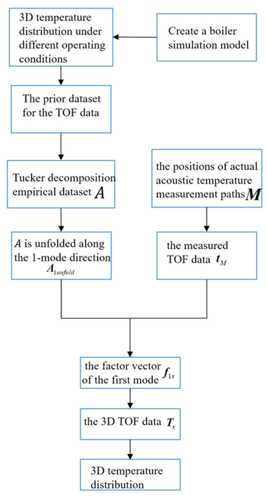
Figure 1.
Flow chart of the 3D reconstruction algorithm.
In the experimental setup, an 8-emitter 24-channel sound wave thermometry system is employed to calculate the TOF data for one layer of temperature distribution. Through the algorithm, the 1-mode direction factor vector is calculated to facilitate the reconstruction of the desired 3D temperature distribution. Consequently, the 3D TOF data are obtained. The final step involves solving the equation set, enabling the acqui-sition of the 3D temperature distribution. This study presents the root mean square error (RMSE) as the evaluation metric to demonstrate the reconstruction performance.
3. Model and Scenario Selection
3.1. Geometric Information for the Boiler Model
In the context of traditional, simple temperature fields generated using MATLAB R2024b, including single-peaked, double-peaked, triple-peaked, symmetric, and asymmetric temperature distributions, extensive research has been conducted to validate various temperature measurement methods. However, these measurement and reconstruction methods often fail to accurately reflect the details of the temperature distribution for complex temperature fields inside a four-corner tangentially fired boiler furnace, leading to a significant number of errors. Therefore, Fluent is utilized in this study to examine the furnace of a four-corner tangential swirl burner and validate the accuracy of the Tucker decomposition-based 3D temperature field reconstruction algorithm.
As shown in Figure 2, the furnace model exhibits specific dimensions. The height of the furnace is 44 m, while its width and depth are 13.26 m and 12.65 m, respectively. The furnace is scaled down to a ratio of 13:1. Moreover, the height and width of the primary and tertiary air nozzles are 45.38 mm and 44.62 mm, respectively. In addition, the height and width of the secondary air nozzles are 25.08 mm and 44.62 mm, respectively.
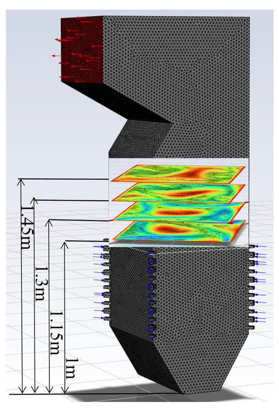
Figure 2.
Schematic diagram of the boiler combustion system and cross-section selection.
The burners are arranged starting at 0.563 m above the bottom of the furnace, and they are divided into two groups. The first group of burners consists of five layers, arranged from bottom to top, as follows: secondary air, primary air, secondary air, primary air, and secondary air. The second group of burners starts at a height of 0.931 m above the bottom of the furnace and comprises six layers, arranged from bottom to top, as follows: secondary air, primary air, secondary air, tertiary air, tertiary air, and secondary air. The angles between the burners and the walls are 42.3° and 45°, respectively.
Using Gambit, the computational domain is meshed with a total of 642,096 grid cells. In this case, the obtained results across all operating conditions demonstrate repeatability and consistency. Hence, the multi-layer 2D temperature distribution can be regarded as one representation of the 3D temperature field. Therefore, at different heights above the upper secondary air, sectional temperature distributions are selected—namely at 1 m, 1.15 m, 1.3 m, and 1.45 m—to serve as the data sources for the 3D temperature field. The section heights are shown in Figure 2, and the temperature distribution data are calculated under various boundary conditions.
3.2. Selection of Prior Dataset and Experimental Dataset Conditions
The quantitative boundary conditions for both the prior dataset and experimental dataset are listed in Table 1, wherein the primary air velocity serves as the variable. For the prior dataset, the primary air velocity starts from 26.5 m/s, with each incremental change of 0.5 m/s representing one prior condition. In particular, a total of 20 prior conditions are simulated, with each condition containing temperature field distributions at four different heights. Consequently, this simulation results in a total of 20 temperature field distributions for various prior conditions. As shown in Figure 3, the positions of the acoustic temperature measurement points, together with the 18 measurement points arranged on each boundary, form a total of 1944 measurement paths. These paths are used to collect 3D TOF data for the four sectional temperatures of the 20 sets of conditions, constituting the prior dataset .

Table 1.
Quantitative boundary conditions for a priori datasets.
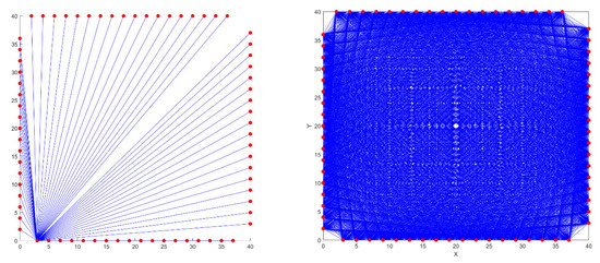
Figure 3.
Positions of acoustic temperature measurement points and paths.
In addition, five experimental conditions are selected with the boundary conditions listed in Table 2 to simulate the temperature field distributions. These five sets of experimental conditions are used to collect 3D TOF data, forming the experimental dataset. Since the boundary conditions for the experimental conditions differ from the prior conditions, the final sampling results in a prior dataset with dimensions of (1944 × 4) × 20 and an experimental dataset with dimensions of (1944 × 4) × 5.
Table 2.
Boundary conditions for the test datasets.
Furthermore, two additional conditions are chosen as validation conditions, with primary air velocities of 36.75 m/s and 37 m/s. These two conditions exceed the range of the prior dataset and are used to test the applicability of the reconstruction algorithm to such conditions.
4. Results and Discussion
4.1. Acoustic Thermometry Reconstruction of Two-Dimensional Temperature Field for Experimental Conditions
Acoustic thermometry is a well-established and reliable temperature measurement technique for power plant boilers that operate continuously. Acoustic thermometry devices are typically installed above the top layer of the burner in practical power plants and boiler applications due to limitations imposed by the combustion chamber and boiler structure. This positioning allows them to obtain temperature distribution information in a 2D plane.
In this study, the traditional acoustic thermometry algorithm is used to reconstruct the temperature field at a height of 1 m in the experimental conditions considered for the mentioned boiler model. According to the arrangement shown in Figure 4a, eight acoustic measurement points are set up, and a receiver and transmitter are arranged at each measurement point. After receiving the sound waves, all receivers move clockwise to the next transmitter position; this process is repeated until all transmitters have emitted sound waves, completing one cycle. This configuration creates an 8-transmitter, 24-channel acoustic thermometry system. Using the relationship between the sound velocity and temperature, the TOF for sound transmission on each channel can be calculated, obtaining TOF data for 24 paths.
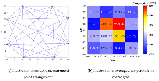
Figure 4.
Schematic diagram of the acoustic measurement point location path and coarse grid temperature. (a) Arrangement and path of acoustic measurement points; (b) coarse grid temperature distribution.
On the one hand, based on the TOF data from the 24 paths, the average temperature across 16 discrete grid points at the height of 1 m can be reconstructed. On the other hand, the TOF data from these 24 paths can be compiled into a single-layer TOF vector, denoted as Tm in Equation (10), to provide a small amount of actual measurement data for the subsequent reconstruction algorithm. Considering condition 2, the average temperature can be solved at a height of z = 1 m within the 16 coarse grid points shown in Figure 4b.
The 16 coarse grid cell temperatures obtained from Figure 4b are treated as the geometric center temperatures of each coarse grid cell. Moreover, third-order polynomial interpolation is applied in the 2D plane. The result regarding the temperature distribution of the planar model is shown in Figure 5b, presenting a reconstruction error rate of 16.11%. The reconstruction results are then compared with the reconstructed temperature field obtained using the new method.
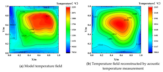
Figure 5.
Temperature distribution at z = 1 m in experimental condition 2. (a) Numerical temperature field; (b) reconstruction of complex temperature field.
As depicted in Figure 5a, the temperature field generated by simulating the combustion of highly volatile coal powder using the Fluent software maintains a skewed single-peaked pattern with a four-corner cut-circle shape, presenting a complex temperature distribution. Traditional acoustic thermometry is constrained by the limited number of measurement points and paths; thus, it only provides a small number of average temperatures for coarse grids, as shown in Figure 4b. Subsequently, the conventional interpolation method is employed to derive finer grid temperatures; however, it also suffers from inherent limitations, such as large extrapolation errors and low smoothness. When reconstructing complex temperature fields using traditional acoustic thermometry interpolation, some essential features can be preserved, but many details are lost, resulting in a considerable number of errors.
The data in Table 3 reveal that the error rates in traditional acoustic reconstruction for the temperature distributions at z = 1 m in the five experimental conditions gradually rise with the increase in the primary air velocity. The temperature field at z = 1 m for experimental condition 2 exhibits the characteristics of a skewed single-peaked symmetric temperature distribution, as observed in Figure 5a. The acoustic thermometry interpolation method performs well in reconstructing symmetric temperature distributions due to its characteristics. Therefore, for experimental condition 2, the reconstructed temperature field at z = 1 m preserves the main features, being consistent with the modeled temperature field. However, the formation of a four-corner cut circle and the single-peaked symmetric temperature distribution are no longer observed as the primary air velocity continues to rise, leading to an increased number of reconstruction errors.
Table 3.
Reconstruction errors for the five operating conditions.
4.2. Reconstruction of a Multi-Layer Temperature Field in Acoustic Thermometry Based on Tucker Decomposition
As shown in the flow chart of the Tucker decomposition reconstruction algorithm, displayed in Figure 1., the first step involves performing Tucker decomposition on the prior dataset to obtain A, followed by unfolding A along the 1-mode direction to obtain . Considering experimental condition 2 and the arrangement of the acoustic thermometry measurement points shown in Figure 4a, the acoustic thermometry path position information and the TOF vector for 24 paths are obtained. Using Equation (10), is calculated; then, Equation (8) is applied to obtain the 3D TOF data to be reconstructed for the four cross-sections in experimental condition 2. Figure 6. presents the errors in the reconstructed TOF data compared to the simulated TOF data derived from the model. The blue clusters represent the reconstruction errors comprising 4 × 1944 TOF values, while the orange scattered points indicate the average reconstruction errors in the TOF data at the four height planes. As can be seen in the graph, the maximum reconstruction error rate in the TOF is approximately 5%, while the average reconstruction error rates in the TOF data at the four height planes range between 0.82% and 1.27%. In particular, the average reconstruction error rate at the z = 1 m height plane is significantly lower than those at the other three height planes. The main reason for this is that the acoustic thermometry path position information M is located at the z = 1 m height plane, and this represents the richest feature information. The Tucker decomposition reconstruction algorithm performs well in reconstructing the TOF data for experimental condition 2.
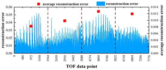
Figure 6.
Average reconstruction error rates regarding TOF data for experimental condition 2.
Using Equations (4) and (5) and the algebraic reconstruction technique (ART), it is possible to reconstruct the TOF data for the four planes. This, in turn, provides the 2D reconstructed temperature distribution for experimental condition 2 at different heights (1 m, 1.15 m, 1.3 m, and 1.45 m). To provide a visual representation, Figure 7 and Figure 8 display the model temperature distribution and the corresponding reconstructed temperature distribution at these heights, respectively. The root means square error (RMSE) for the temperature reconstruction in experimental condition 2 is 6.4035%, and the reconstruction time is 4.38 s.
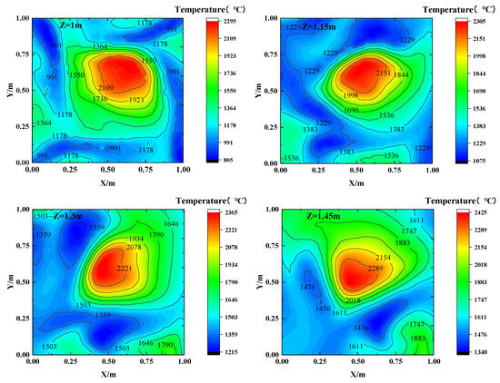
Figure 7.
Modeled temperature field for experimental condition 2.
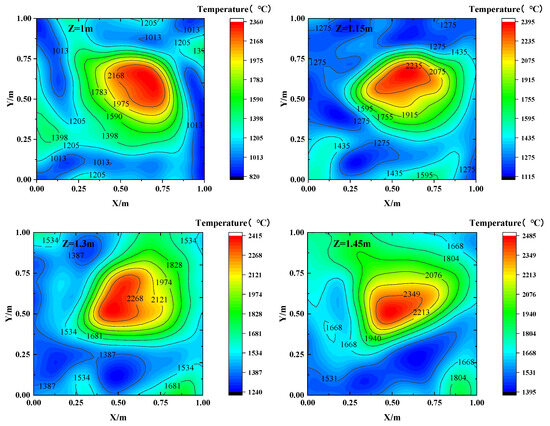
Figure 8.
Multi-layer reconstruction of temperature field based on Tucker decomposition acoustic thermometry for experimental condition 2.
Comparing the reconstructed temperature field at z = 1 m, obtained via Tucker decomposition and shown in Figure 8, with the reconstructed temperature field obtained via acoustic thermometry and shown in Figure 5b, it can be seen that Tucker decomposition-based reconstruction yields more accurate and clearly differentiated results. In addition, it can sufficiently reflect the main temperature region and capture the fine details around the edges, thereby reducing the number of errors introduced compared to acoustic thermometry interpolation and minimizing edge errors. Compared to traditional acoustic thermometry interpolation, Tucker decomposition improves the accuracy and quality of the temperature reconstruction.
As evidenced by Figure 7 and Figure 8, the measurement points are evenly distributed at a height of z = 1 m due to the arrangement of the measurement points, reflecting that used in actual power station boilers for acoustic thermometry. Consequently, the temperature field reconstruction at z = 1 m yields the best results. However, some information loss occurs during temperature reconstruction on the other planes, leading to errors in certain details, although the main temperature characteristics are retained. Although placing the measurement points on a single plane introduces some errors, the proposed reconstruction algorithm maintains a high level of accuracy and reliability.
Compared to traditional acoustic thermometry, the reconstruction algorithm significantly improves the reconstruction accuracy for a single plane and overcomes the limitations of traditional acoustic thermometry, which is restricted to the measurement of a single plane. It is also worth noting that more temperature information is acquired when generalizing the measurement data from a single plane to other planes.
Figure 9 illustrates the reconstruction errors and time consumption for the five distinct experimental conditions. Notably, the reconstruction time for all five conditions is approximately 4 s, and the choice of conditions has a minimal impact on the reconstruction time. Regarding the reconstruction accuracy, for these experimental conditions, within the range of boundary conditions present in the prior dataset, the reconstruction error rate ranges from 4% to 9%. However, it is approximately 8.4% for conditions beyond the range of the prior dataset.
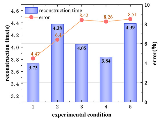
Figure 9.
Time consumption and error rate during the reconstruction of the experimental working conditions.
In the case of the boiler model examined in this study, the design condition corresponds to a first air velocity of 27 m/s. Deviations in the first air velocity from the design condition lead to a more complex temperature distribution. Experimental conditions 3, 4, and 5 exhibit notable deviations from the design condition in terms of the first air velocity; specifically, conditions 4 and 5 exhibit boundary conditions that exceed the range of the prior dataset. Consequently, the reconstruction error rates for conditions 4 and 5 increase slightly, but they remain within a relatively small range, at approximately 8.4%.
In order to validate the difference between the TOF-based Tucker decomposition reconstructed temperature field and the point measurement-based Tucker decomposition reconstructed temperature field, we carried out the four-layer temperature field constructed using CFD in Section 3.1 in the previous Tucker decomposition reconstruction of the temperature field study of point measurements as the measurement data, 20 measurement point locations are shown in Figure 10, Case 2 was selected as the comparison case, and the temperature field reconstructed using point measurements is shown in Figure 11, which shows that in the Z = 1 m cross-section where the distribution of the measurement points is more densely distributed, the reconstruction effect is better. It can be seen that the reconstruction effect is better in the Z = 1 m section where the distribution of measurement points is denser, but compared with the temperature field reconstructed using TOF data in Figure 8, the reconstruction error of the temperature distribution in the high-temperature region is larger, and the reconstruction of the remaining three sections has a larger error, and the root-mean-square error for the reconstruction of Case 2 using point measurements is 11.2%. By comparison, we can find that the temperature field obtained from the Tucker decomposition reconstruction based on acoustic tomography is overall better than the reconstructed temperature field based on point measurements.
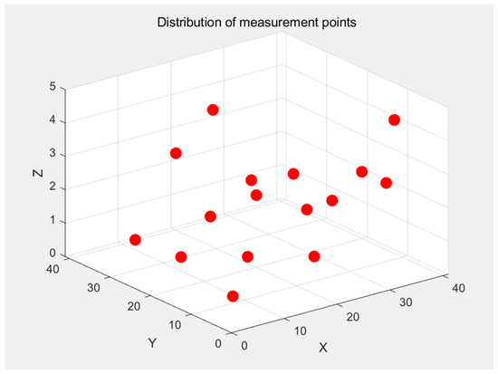
Figure 10.
Distribution of measuring points for Tucker decomposition point measurement.
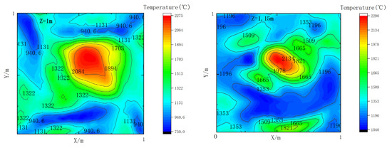
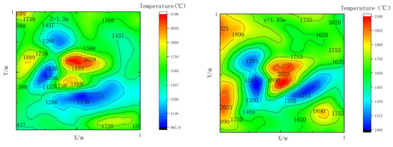
Figure 11.
Multi-layer temperature field reconstruction based on point measurements of the Tucker decomposition (Experimental Condition 2).
In summary, the Tucker decomposition algorithm demonstrates stable and reliable temperature field reconstruction for different conditions.
4.3. Verification of the Algorithm’s Noise Resistance
In practical time-of-flight (TOF) measurements, sampling errors are likely, so we introduce 1% Gaussian noise into the measured TOF data. The reconstructed temperature field at a height of 1 m and the error distribution after the addition of noise are shown in Figure 12a,b. From Figure 12a, it is evident that significant errors occur in the areas with the steepest temperature gradients, as these regions are more sensitive to noise. Additionally, the TOF-based temperature field reconstruction exhibits limitations in high-temperature areas. However, the number of errors in other areas is relatively small, and the reconstructed temperature field maintains the primary trends seen in the original field, accurately reflecting both the temperature gradients and regions. As shown in Figure 12c, the relative error rates are mostly within 10%, with only a few areas experiencing larger numbers of errors. Compared to the temperature field reconstructed via interpolation from two-dimensional acoustic temperature measurements using 8 measurement points and 24 channels, the one reconstructed using our algorithm still shows good results. This indicates that the algorithm possesses strong resistance to noise.
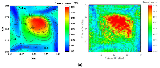
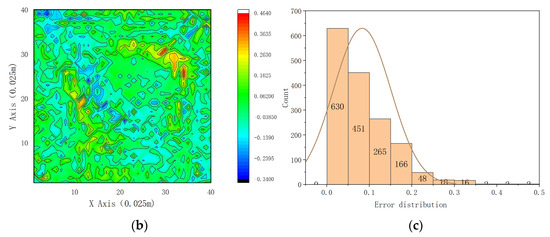
Figure 12.
Reconstruction error distribution in experimental condition 2 with Gaussian noise at 1 m. (a) Simulation (left) and reconstruction (right) of temperature distribution at z = 1 m in experimental condition 2. (b) Reconstruction error position distribution. (c) Numerical distribution of reconstruction error.
4.4. Reconstruction of a 3D Temperature Field in Acoustic Thermometry Based on Tucker Decomposition
In our model design, we utilize a grid of 40 × 40 × 31 temperature nodes to cover a space ranging from 1 to 1.45 m in height, with each node measuring 0.025 × 0.025 × 0.025 cubic meters. We apply the Tucker decomposition algorithm to reconstruct these 31 sections. Figure 13. displays the temperature field of the model, the reconstruction results, and the errors for experimental condition 5. Dsespite the loss of some details, the reconstructed temperature field retains the main characteristics of the model. The error range for most of the reconstructed temperature field lies between −100 and 200 °C, indicating that it is feasible to characterize the three-dimensional temperature field by reconstructing all sections. Notably, after an increase in the primary airspeed, the temperature field gradually loses its unique squared–circular shape, showing reduced regularity under higher primary air speeds compared to lower ones, as well as greater reconstruction errors in irregular high-temperature areas. The significant reconstruction error rate in experimental condition 5 is partly due to its absence in the prior dataset and partly due to the shape deviation in the temperature field caused by the increased primary airspeed. Therefore, categorizing the data and selecting the prior dataset based on the experimental conditions might represent an effective strategy to enhance the reconstruction results.
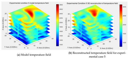
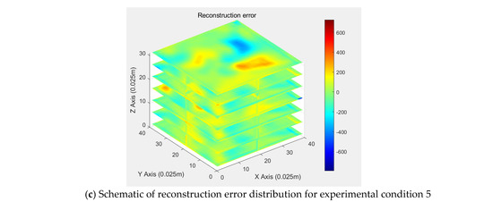
Figure 13.
Reconstruction of 3D temperature distribution in experimental condition 5.
5. Conclusions and Outlook
In this study, a novel 3D temperature field reconstruction algorithm based on Tucker’s decomposition and acoustic temperature measurement is proposed, which greatly improves the accuracy and reliability of acoustic temperature measurements in complex 3D temperature fields and reduces the reconstruction error by 10–20% compared to the traditional method, and by about 6% compared to the fixed-measurement Tucker’s decomposition reconstruction algorithm. The reconstruction process takes about 4 s and is suitable for real-time industrial applications. The algorithm is robust to Gaussian noise and performs well in temperature fields beyond the range of the previous dataset, demonstrating its adaptability to various operating conditions. The method provides a cost-effective solution for three-dimensional temperature monitoring in coal-fired power plants, supporting combustion optimization and flexible load adjustment under carbon-neutral targets.
Although the proposed algorithm provides significant improvements in 3D temperature field reconstruction, some limitations should be recognized: the algorithm relies heavily on CFD-generated a priori datasets, which may not fully capture the stochastic variations (e.g., coal particle fluctuations, ash deposition) in the actual boiler environment. This may limit its generalizability to real-world applications. The study assumes that the distribution of acoustic measurement points is ideal. In industrial environments, the placement of sensors may be limited by physical space, resulting in sparse data coverage in certain areas and reduced reconstruction accuracy. Noise immunity tests are limited to Gaussian noise. In the real world, noise may exhibit spatial correlation or non-stationary behavior (e.g., local high-temperature distortion), which may affect the robustness of the algorithm.
To address limitations and further improve the applicability of the proposed methodology, future research directions include conducting field experiments at an operating coal-fired power plant to validate the algorithm’s performance under realistic noise and interference conditions, developing strategies to optimize sensor locations to maximize data coverage and minimize reconstruction errors in space-constrained environments; combining Tucker decomposition with deep learning models (e.g., CNNs or transformers) to improve detail preservation and robustness to complex noise patterns; investigating the applicability of the algorithm in other industrial scenarios, such as for 3D temperature monitoring critical waste incinerators and aerospace combustion chambers.
Author Contributions
Conceptualization, L.A.; methodology, S.Z.; investigation, P.Y. and G.S.; writing—original draft preparation, J.Y. and P.Y.; writing—review and editing, J.Y. and P.Y. All authors have read and agreed to the published version of the manuscript.
Funding
This research received no external funding.
Institutional Review Board Statement
Not applicable.
Informed Consent Statement
Informed consent was obtained from all subjects involved in the study.
Data Availability Statement
Dataset available upon request from the authors.
Conflicts of Interest
The authors declare no conflicts of interest.
References
- Swift, G.W. Analysis and performance of a large thermoacoustic engine. J. Acoust. Soc. Am. 1992, 92, 1551–1563. [Google Scholar] [CrossRef]
- Yoshiba, F.; Hanai, Y.; Watanabe, I.; Shirai, H. Methodology to evaluate contribution of thermal power plant flexibility to power system stability when increasing share of renewable energies: Classification and additional fuel cost of flexible operation. Fuel 2021, 292, 120352. [Google Scholar] [CrossRef]
- Zhang, S.; Shen, G.; An, L.; Niu, Y. Online monitoring of the two-dimensional temperature field in a boiler furnace based on acoustic computed tomography. Appl. Therm. Eng. 2015, 75, 958–966. [Google Scholar] [CrossRef]
- Śladewski, Ł.; Wojdan, K.; Świrski, K.; Janda, T.; Nabagło, D.; Chachuła, J. Optimization of combustion process in coal-fired power plant with utilization of acoustic system for in-furnace temperature measurement. Appl. Therm. Eng. 2017, 123, 711–720. [Google Scholar] [CrossRef]
- Norton, S.J. Tomographic reconstruction of 2-D vector fields: Application to flow imaging. Geophys. J. Int. 1989, 97, 161–168. [Google Scholar] [CrossRef]
- Wilson, D.K. Acoustic Tomographic Monitoring of the Atmospheric Boundary Layer. Master’s Thesis, The Pennsylvania State University, University Park, PA, USA, 1992. [Google Scholar]
- Bao, Y.; Jia, J. Online time-resolved reconstruction method for acoustic tomography system. IEEE Trans. Instrum. Meas. 2019, 69, 4033–4041. [Google Scholar] [CrossRef]
- Onunwor, E.; Reichel, L. On the computation of a truncated SVD of a large linear discrete ill-posed problem. Numer. Algorithms 2017, 75, 359–380. [Google Scholar] [CrossRef]
- Li, Y.-Q.; Wang, Y.-W.; Guan, X.-F.; Zhou, H.-C.; Ma, X.-L. A wavelet model on reconstructing complex aerodynamic field in furnace with acoustic tomography. Measurement 2020, 157, 107669. [Google Scholar] [CrossRef]
- Schwarz, A. Three-Dimensional Reconstruction of Temperature and Velocity Fields in a Furnace. Part. Part. Syst. Charact. 1995, 12, 75–80. [Google Scholar] [CrossRef]
- Lu, H.B.; Sun, W.H.; Li, Z.H. Research on Reconstruction Algorithm of Temperature Field by Acoustic Measurement in Boiler. Adv. Mater. Res. 2012, 424–425, 1305–1308. [Google Scholar] [CrossRef]
- Bao, Y.; Jia, J.; Polydorides, N. Real-time temperature field measurement based on acoustic tomography. Meas. Sci. Technol. 2017, 28, 074002. [Google Scholar] [CrossRef]
- Kong, Q.; Jiang, G.; Liu, Y.; Sun, J. 3D high-quality temperature-field reconstruction method in furnace based on acoustic tomography. Appl. Therm. Eng. 2020, 179, 115693. [Google Scholar] [CrossRef]
- Zhang, J.; Qi, H.; Wu, J.; He, M.; Ren, Y.; Su, M.; Cai, X. Numerical and experimental investigation of many-objective optimization for efficient temperature and velocity fields reconstruction via acoustic tomography. Int. J. Therm. Sci. 2023, 193, 108536. [Google Scholar] [CrossRef]
- Ma, T.; Liu, Y.; Cao, C. Neural networks for 3D temperature field reconstruction via acoustic signals. Mech. Syst. Signal Process. 2019, 126, 392–406. [Google Scholar] [CrossRef]
- Vecherin, S.N.; Ostashev, V.E.; Ziemann, A.; Wilson, D.K.; Arnold, K.; Barth, M. Tomographic Reconstruction of Atmospheric Turbulence with the Use of Time-Dependent Stochastic Inversion. J. Acoust. Soc. Am. 2007, 122, 1416–1425. [Google Scholar] [CrossRef]
- Modliński, N.; Madejski, P.; Janda, T.; Szczepanek, K.; Kordylewski, W. A validation of computational fluid dynamics temperature distribution prediction in a pulverized coal boiler with acoustic temperature measurement. Energy 2015, 92, 77–86. [Google Scholar] [CrossRef]
- Bian, C.; Huang, J.; Sun, R. Numerical optimization of combustion and NOX emission in a retrofitted 600MWe tangentially-fired boiler using lignite. Appl. Therm. Eng. 2023, 226, 120228. [Google Scholar] [CrossRef]
- Azizinasab, B.; Hasanzadeh, R.P.R.; Hedayatrasa, S.; Kersemans, M. Defect detection and depth estimation in CFRP through phase of transient response of flash thermography. IEEE Trans. Ind. Inform. 2021, 18, 2364–2373. [Google Scholar] [CrossRef]
- Jiang, G.; Kang, M.; Cai, Z.; Wang, H.; Liu, Y.; Wang, W. Online reconstruction of 3D temperature field fused with POD-based reduced order approach and sparse sensor data. Int. J. Therm. Sci. 2022, 175, 107489. [Google Scholar] [CrossRef]
- Le, T.T.; Abed-Meraim, K.; Trung, N.L.; Hafiane, A. A novel recursive least-squares adaptive method for streaming tensor-train decomposition with incomplete observations. Signal Process. 2023, 216, 109297. [Google Scholar] [CrossRef]
- Schneider, R.; Uschmajew, A. Approximation rates for the hierarchical tensor format in periodic Sobolev spaces. J. Complex. 2014, 30, 56–71. [Google Scholar] [CrossRef]
- Gong, W.; Huang, Z.; Yang, L. Accurate regularized Tucker decomposition for image restoration. Appl. Math. Model. 2023, 123, 75–86. [Google Scholar] [CrossRef]
- Luu, T.H.; Maday, Y.; Guillo, M.; Guérin, P. A new method for reconstruction of cross-sections using Tucker decomposition. J. Comput. Phys. 2017, 345, 189–206. [Google Scholar] [CrossRef]
- Hu, Y.; Cui, F.; Zhao, Y.; Li, F.; Cao, S.; Xuan, F.-Z. Tensor robust principal component analysis based on Bayesian Tucker decomposition for thermographic inspection. Mech. Syst. Signal Process. 2023, 204, 110761. [Google Scholar] [CrossRef]
- Kilmer, M.E.; Braman, K.; Hao, N.; Hoover, R.C. Third-order tensors as operators on matrices: A theoretical and computational framework with applications in imaging. SIAM J. Matrix Anal. Appl. 2013, 34, 148–172. [Google Scholar] [CrossRef]
- Wang, J.; Liu, M.; Wang, X.; Liu, T.; Xie, X. Prediction of head-related transfer function based on tensor completion. Appl. Acoust. 2020, 157, 106995. [Google Scholar] [CrossRef]
- Tucker, A.L.; Edmondson, A.C.; Spear, S. When problem solving prevents organizational learning. Probl. Meas. Change 1963, 15, 122–137. [Google Scholar] [CrossRef]
- Zhang, G.; Zheng, X.; Liu, S.; Chen, M.; Wang, C.; Wang, X. Three-dimensional wind velocity reconstruction based on tensor decomposition and CFD data with experimental verification. Energy Convers. Manag. 2022, 256, 115322. [Google Scholar] [CrossRef]
- Zhang, G.; Zheng, X.; Liu, S.; Chen, M. Three-dimensional wind field reconstruction using tucker decomposition with optimal sensor placement. Energy 2022, 260, 125098. [Google Scholar] [CrossRef]
- Liu, Z.; Liu, S.; Chen, M.; Zhang, Y.; Yao, P. Application of Tucker Decomposition in Temperature Distribution Reconstruction. Appl. Sci. 2022, 12, 2749. [Google Scholar] [CrossRef]
- Liu, Z.; Liu, S.; Zhang, Y.; Yao, P. Reconstruction Optimization Algorithm of 3D Temperature Distribution Based on Tucker Decomposition. Appl. Sci. 2022, 12, 10814. [Google Scholar] [CrossRef]
- Othmani, C.; Dokhanchi, N.S.; Merchel, S.; Vogel, A.; Altinsoy, M.E.; Voelker, C.; Takali, F. Acoustic tomographic reconstruction of temperature and flow fields with focus on atmosphere and enclosed spaces: A review. Appl. Therm. Eng. 2023, 223, 119953. [Google Scholar] [CrossRef]
- Zhang, W.; Jiang, G.; Sun, J.; Liu, Y. Measurement the 3D temperature distribution in the combustion zone using acoustic tomography and nolinear wavefont tracing. Measurement 2024, 229, 114439. [Google Scholar] [CrossRef]
- Zhong, Q.; Chen, Y.; Zhu, B.; Liao, S.; Shi, K. A temperature field reconstruction method based on acoustic thermometry. Measurement 2022, 200, 111642. [Google Scholar] [CrossRef]
- Barathula, S.; Chaitanya, S.K.; Alapati, J.K.; Srinivasan, K. Precise temperature reconstruction in acoustic pyrometry: Impact of domain discretization and transceiver count. Appl. Therm. Eng. 2023, 238, 122009. [Google Scholar] [CrossRef]
- Chaitanya, S.; Alapati, J.K.; Srinivasan, K. Evaluation of regularization methods for acoustic pyrometry. Measurement 2022, 198, 111356. [Google Scholar] [CrossRef]
- Li, R.; Pan, Z.; Wang, Y.; Wang, P. The correlation-based tucker decomposition for hyperspectral image compression. Neurocomputing 2021, 419, 357–370. [Google Scholar] [CrossRef]
- Qin, L.; Liu, S.; Kang, Y.; Yan, S.A.; Schlaberg, H.I.; Wang, Z. Wind velocity distribution reconstruction using CFD database with Tucker decomposition and sensor measurement. Energy 2019, 167, 1236–1250. [Google Scholar] [CrossRef]
Disclaimer/Publisher’s Note: The statements, opinions and data contained in all publications are solely those of the individual author(s) and contributor(s) and not of MDPI and/or the editor(s). MDPI and/or the editor(s) disclaim responsibility for any injury to people or property resulting from any ideas, methods, instructions or products referred to in the content. |
© 2025 by the authors. Licensee MDPI, Basel, Switzerland. This article is an open access article distributed under the terms and conditions of the Creative Commons Attribution (CC BY) license (https://creativecommons.org/licenses/by/4.0/).