The Electromagnetic Field Analytical Solution Analysis to Downhole Current Injection Ranging

Abstract

As the final crucial line of defense against well blowout accidents, the implementation of the relief well scheme facilitates the swiftest possible rescue of the target well, thereby minimizing economic losses and enhancing production efficiency. Among them, the relative distance and orientation determination between the relief well and the accident well becomes the key to the rapid intersection and connection of the two wells. However, the inaccessibility of the accident well due to safety factors makes it challenging to accurately determine the relative position of the two wells. The current injection method has now been proved to be able to achieve relief well detection, and some signal processing methods are necessary for optimizing the detection performance. In the process of signal characterization, analytical methods show many advantages due to their direct relevance to the principles of electromagnetic theory. To provide an effective theoretical basis for the optimization of relief well detection methods, this paper proposes an analytical solution to the corresponding electromagnetic field distribution for current injection detection scheme. Based on the principle of the current injection detection, the signal model is constructed, and the electromagnetic distribution expression is deduced. Then, the adaptability of the analytical solution obtained under different physical parameters is investigated. Moreover, the reliability and validity of the proposed analytical solution are validated by comparing the results with those obtained from finite element numerical simulations, thus providing a theoretical basis for subsequent signal processing and method optimization.

1. Introduction

Major accidents, such as oil spills, well blowouts, and well overflows, can cause significant damage to oil and gas resources, lead to the destruction of operating equipment, the scrapping of wells, and result in severe environmental pollution. In response to these problems, how to carry out a rapid and efficient rescue after the accident has become the focus of attention. Currently, the implementation of a relief well is regarded as the most effective method for addressing well blowout accidents [1,2,3]. With the growing emphasis on environmental and safety protection, relief wells have become a critical last-resort measure for controlling inaccessible blowout wells, playing a vital role in ensuring drilling safety. In the event of a sudden blowout or the failure of conventional well-killing methods, drilling a relief well is necessary to promptly regain control and prevent severe consequences, including environmental pollution and significant economic losses. In this process, the relief well intersects and connects with the target well, allowing high-density pressurized fluid to be injected into the relief well to control the blowout in the accident well [4,5,6]. For achieving a rapid and successful connection, it is crucial to determine the relative position between the two wells.

In real-world applications, accurately determining the distance between two wells is highly challenging due to the unpredictable and harsh downhole conditions, along with the strict reliability standards required to ensure a successful relief well intersection and minimize potential losses [3]. Traditional inclinometer tools exhibit a notable decline in detection accuracy as drilling depth increases, often failing to meet the necessary ranging precision [7]. To improve accuracy and support real-time control and guidance in drilling operations, several magnetic ranging techniques have been introduced, including passive magnetic ranging (PMR) and active magnetic ranging (AMR) [8,9,10,11]. PMR estimates the relative position of the target well by detecting and analyzing magnetic field disturbances induced by magnetic structures, such as casing or drill pipes, within the target well using surface-based software systems [12]. Since PMR relies on the residual magnetism, it typically requires no additional drilling hardware and is relatively straightforward to operate. However, this method is highly susceptible to environmental factors. When the relief well is located at a considerable distance from the target well or when sections of the casing exhibit minimal residual magnetism, the magnetic field disturbances detected by the magnetometer in the relief well become exceedingly weak. Consequently, the ranging accuracy of PMR tools degrades significantly under such conditions [13].

Unlike PMR, which relies on residual magnetic fields, AMR utilizes an excitation source along with high-sensitivity sensors to generate strong electromagnetic signals. This enhancement allows for greater detection distances and improved accuracy [14,15]. However, AMR applications are constrained to specific conditions and are generally classified into two categories based on the accessibility of the target well, access-dependent AMR (AD-AMR) and access-independent AMR (AI-AMR) [16]. Common AD-AMR systems include the magnetic guidance tool (MGT) [17], the single wire guidance (SWG) tool [18], and rotating magnet ranging service (RMRS) [19]. Although these systems provide precise ranging, they require an excitation source or detection device to be placed within the target well, which is often impractical in the real-world drilling environment. The current injection method, as an effective method for the detection and localization of the relief well, is able to achieve a large detection distance [15]. This method mainly uses the downhole electrode to inject a large current into the stratum, which in turn forms a converging current on the accident well casing, and obtains the relative positions between the relief well and the accident well by measuring the alternating magnetic field generated by the converging current in the relief well [20,21,22].

While the effectiveness of the above detection methods has been verified, improving detection accuracy and increasing detection range have become the primary research focuses for the precise positioning of the target well during the relief well operation. Several researchers have carried out simulations and analyses on the relief wells detection systems [23,24]. Hao et al. [13] analyzed the changing law of converging current and measured magnetic field with geological parameters according to the basic principle of current injection [25]. Further, Zhang et al. used a numerical simulation approach to analyze in detail the factors influencing the detection performance of current injection ranging [26]. Moreover, Dang et al. employed the finite element method to simulate the current density and magnetic field distribution in the entire measured area. They also analyzed the impact of electrode placement on detection performance and proposed an optimization scheme along with a high-precision ranging algorithm for practical applications [27].

Although numerical simulation methods are widely used because of their adaptability to complex models, analytical methods perform better in signal characterization because of their direct relevance to electromagnetic problems [28,29,30]. Specifically, using analytical methods to solve the electromagnetic response allows for a deeper analysis of the structural characteristics of electromagnetic signals and the behavior of electromagnetic fields. This approach provides a reliable theoretical foundation for further signal processing and method optimization. In light of this, an analytical solution for the electromagnetic field distribution in relief well detection is proposed in this paper. Focusing on the detection principle of current injection, the signal model is developed, and the analytical solution to the electromagnetic problem is derived from theoretical formulas. Based on this, the structural and electromagnetic parameters of the detection system are varied, and the adaptability of the proposed analytical solution, along with the influencing factors, are examined. Finally, the effectiveness of the proposed analytical solution is validated through numerical simulation results with a comparison analysis using finite element methods.

The remainder of this paper is organized as follows. In Section 2, the signal model for the current injection relief well detection is introduced, and the derivation of the electromagnetic equations and the acquisition of the analytical solution are completed. In Section 3, the variations in the analytical solution under different physical parameters are demonstrated, and the effectiveness of the proposed method is proved through comparative analyses. Finally, Section 4 concludes the paper.

2. Signal Model and Electromagnetic Field Distribution Analysis

2.1. Signal Model

A standard current-injection ranging system, as depicted in Figure 1, consists of a surface electrode, a downhole electrode, and a sensing tool with magnetometers. In operation, the downhole electrode introduces a low-frequency AC current into the surrounding formation, where it disperses and weakens over distance. Since the conductivity of the target well (casing) is considerably greater than that of the stratum, the current is disturbed by short-circuit effects. A low-frequency alternating magnetic field will be generated when the current converges on the target well. Sensors positioned in the relief well detect this magnetic field, allowing for the estimation of the relative distance between two wells [31].

To achieve accurate well ranging results, the electromagnetic field distribution around the target well needs to be calculated. Nevertheless, since the analytical solution for the multi-layer medium cannot be obtained, the downhole current injection model utilized in Figure 1 must be further simplified. Considering that the conductivity of the target well is substantially higher than that of the stratum and relief well, our work simplifies the multi-layer model in Figure 1 to a two-layer model shown in Figure 2, where the injection current is modeled as a point current.

Based on the two-layer model, the distribution of the primary and secondary electromagnetic fields can be expressed in an analytical form. Firstly, the primary electromagnetic field generated in the active region is calculated.

2.2. The Primary Electric Potential in Active Region Analysis

According to Maxwell’s equation, the primary electric potential in the active region satisfies Poisson’s equation [32], as follows:

$${\nabla }^2{V}_1=-{\displaystyle \frac{I}{{\sigma }_1}}\delta (\mathit{r}),$$

(1)

where ${\nabla }^2$ is the Laplace operator; $V_1$ denotes the primary electric potential; $I\delta ({\mathit{r}}_0)$ represents the point current source; $\delta (•)$ is the Dirac function; ${\mathit{r}}_0=({\rho }_0,{\phi }_0,z_0)$ is the position of the point current source; and ${\sigma }_1$ denotes the conductivity in the active region. The solution to this equation is as follows:

$$V_1={\displaystyle {\int }_0^{+\infty }f\left(\lambda \right)K_0\left(\lambda \rho \right)cos(\lambda z}) d\lambda ,$$

(2)

where $f\left(\lambda \right)={\displaystyle \frac{I}{2{\pi }^2{\sigma }_1}}$, $K_{\mathrm{i}}\left(•\right)$ denotes the i-order modified Bessel functions of type 2 [33]. By employing the cylindrical coordinate system, when the point source is located at $({\rho }_0,{\phi }_0,z_0)$, the primary electric potential can be represented as follows:

$$V_1={\displaystyle \frac{I}{4{\pi }^2{\sigma }_1}}{\displaystyle {\int }_{-\infty }^{+\infty }{K}_0\left(\lambda \left|\rho -{\rho }_0\right|\right)}{e}^{i\lambda \left(z-z_0\right)} d\lambda .$$

(3)

In addition, according to the addition formula for the modified Bessel function, we have

$$K_0\left(\lambda \left|\rho -{\rho }_0\right|\right)=\left\{\begin{array}{c}{\displaystyle \sum _{m=-\infty }^{\infty }{I}_m\left(\lambda {\rho }_0\right)K_m\left(\lambda \rho \right)e^{im\left(\phi -{\phi }_0\right)},\left(\rho >{\rho }_0\right)}\\ {\displaystyle \sum _{m=-\infty }^{\infty }{K}_m\left(\lambda {\rho }_0\right)I_m\left(\lambda \rho \right)e^{im\left(\phi -{\phi }_0\right)},\left(\rho <{\rho }_0\right).}\end{array}\right.$$

(4)

Hence, Equation (3) can be modified as follows:

$$V_1=\left\{\begin{array}{c}{\displaystyle \frac{I}{4{\pi }^2{\sigma }_1}}{\displaystyle {\int }_{-\infty }^{+\infty }{I}_0\left(\lambda {\rho }_0\right)K_0\left(\lambda \rho \right)e^{i\lambda \left(z-z_0\right)}} d\lambda ,\left(\rho >{\rho }_0\right)\\ {\displaystyle \frac{I}{4{\pi }^2{\sigma }_1}}{\displaystyle {\int }_{-\infty }^{+\infty }{I}_0\left(\lambda {\rho }_0\right)K_0\left(\lambda \rho \right)e^{i\lambda \left(z-z_0\right)}} d\lambda ,\left(\rho <{\rho }_0\right).\end{array}\right.$$

(5)

According to the model, the point current source is located in the outermost layer, so the scenario $\rho <{\rho }_0$ needs to be considered and the primary electric potential in the active region is expressed as follows:

$$V_1={\displaystyle \frac{I}{4{\pi }^2{\sigma }_1}}{\displaystyle {\int }_{-\infty }^{+\infty }{I}_0\left(\lambda {\rho }_0\right)K_0\left(\lambda \rho \right)} e^{i\lambda \left(z-z_0\right)} d\lambda .$$

(6)

2.3. The Secondary Electric Potential Analysis

Under the quasi-stationary field assumption, the secondary electric potential satisfies the homogeneous Laplace equation, which can be represented as follows:

$${\nabla }^2{V}_2=0.$$

(7)

By utilizing the cylindrical coordinate system, the Laplace equation can be expanded as follows:

$${\displaystyle \frac{1}{\rho }}{\displaystyle \frac{\partial }{\partial \rho }}\left(\rho {\displaystyle \frac{\partial V_2}{\partial \rho }}\right)+{\displaystyle \frac{1}{{\rho }^2}}{\displaystyle \frac{{\partial }^2{V}_2}{\partial {\phi }^2}}+{\displaystyle \frac{{\partial }^2{V}_2}{\partial z^2}}=0.$$

(8)

Assume that the solution is separable, substituting $V_2=R\left(\rho \right)\Phi \left(\phi \right)Z\left(z\right)$ into Equation (8) yields

$${\nabla }^2{V}_2={\displaystyle \frac{1}{\rho }}{\displaystyle \frac{\partial }{\partial \rho }}\left(\rho {\displaystyle \frac{\partial V_2}{\partial \rho }}\right)+{\displaystyle \frac{1}{{\rho }^2}}{\displaystyle \frac{{\partial }^2{V}_2}{\partial {\phi }^2}}+{\displaystyle \frac{{\partial }^2{V}_2}{\partial z^2}}={\displaystyle \frac{1}{\rho }}\left(R^{\prime }\Phi Z+\rho R^{″}\Phi Z\right)+{\displaystyle \frac{1}{{\rho }^2}}R{\Phi }^{″}Z+R\Phi Z^{″}=0,$$

(9)

where the superscripts $\prime$ and $″$ represent the first and second derivatives of a function. Let ${\displaystyle \frac{\rho R^{\prime }\Phi +{\rho }^2{R}^{″}\Phi +R{\Phi }^{″}}{{\rho }^{2}R\Phi }}=-{\displaystyle \frac{Z^{″}}{Z}}={\lambda }^2$, where $\lambda$ is an introduced variable. Separate Equation (9) into the following two equations:

$$-{\displaystyle \frac{Z^{″}}{Z}}={\lambda }^2,$$

(10)

$${\displaystyle \frac{\rho R^{\prime }\Phi +{\rho }^2{R}^{″}\Phi +R{\Phi }^{″}}{{\rho }^{2}R\Phi }}={\lambda }^2.$$

(11)

The solution to Equation (10) is $Z\left(z\right)=e^{\pm i\lambda z}$. To solve Equation (11), it also needs to be separated into two equations as ${\displaystyle \frac{{\rho }^2{R}^{″}+\rho R^{\prime }-{\lambda }^2{\rho }^{2}R}{R}}=-{\displaystyle \frac{{\Phi }^{″}}{\Phi }}=m^2$. Obviously, the solution to $-{\displaystyle \frac{{\Phi }^{″}}{\Phi }}=m^2$ is $\Phi \left(\phi \right)=e^{\pm im\phi }$, while the equation ${\displaystyle \frac{{\rho }^2{R}^{″}+\rho R^{\prime }-{\lambda }^2{\rho }^{2}R}{R}}=m^2$ needs to be further analyzed. Here, the variable transformation is used. Let $x=\lambda \rho$, ${\displaystyle \frac{{\rho }^2{R}^{″}+\rho R^{\prime }-{\lambda }^2{\rho }^{2}R}{R}}=m^2$ can be transformed into

$$x^2{\displaystyle \frac{{\partial }^{2}R\left(\frac{x}{\lambda }\right)}{\partial x^2}}+x{\displaystyle \frac{\partial R\left(\frac{x}{\lambda }\right)}{\partial x}}-\left(x^2+m^2\right)R=0,$$

(12)

which is similar to the modified Bessel equation. The standard Bessel function and the modified Bessel function are the solutions of the standard Bessel equation and the modified Bessel equation, respectively, and this distinction should be made. The only difference between the standard Bessel equation and the modified Bessel equation is the opposite sign of the non-derivative term. Since they have numerous solutions, they have been classified accordingly. More details can be seen in [33]. Equation (12) has exactly the same form as the Bessel equation, with the only difference being that the independent variable in $R\left({\displaystyle \frac{x}{\lambda }}\right)$ is ${\displaystyle \frac{x}{\lambda }}$ rather than $x$. Hence, it is concluded that the solution to Equation (12) is a Bessel function that can be expressed as follows:

$$R\left(\rho \right)=A{I}_0\left(\lambda \rho \right)+B{K}_0\left(\lambda \rho \right),$$

(13)

where $A$ and $B$ are boundary coefficients. Since the solution is a periodic function of the azimuth angle, m is an integer. Additionally, the eigenvalue of Equation (12) can take values over the entire real number range. Therefore, the secondary potential is expressed as follows:

$$V_2={\displaystyle {\int }_{-\infty }^{+\infty }{e}^{i\lambda z}}\left[A{I}_0\left(\lambda \rho \right)+B{K}_0\left(\lambda \rho \right)\right] d\lambda .$$

(14)

After obtaining the primary electric potential and the secondary electric potential and transforming the primary electric potential and the secondary electric potential into the same form, the total electric potential in the active region and passive region can be obtained as follows:

$$V_2={\displaystyle \frac{I}{4{\pi }^2{\sigma }_1}}{\displaystyle {\int }_{-\infty }^{+\infty }{K}_0\left(\lambda {\rho }_0\right)\left[I_0\left(\lambda \rho \right)+A_1{I}_0\left(\lambda \rho \right)+B_1{K}_0\left(\lambda \rho \right)\right]e^{i\lambda \left(z-z_0\right)} }d\lambda .$$

(15)

$$V_p={\displaystyle \frac{I}{4{\pi }^2{\sigma }_2}}{\displaystyle {\int }_{-\infty }^{+\infty }{K}_0\left(\lambda {\rho }_0\right)\left[A_2{I}_0\left(\lambda \rho \right)+B_2{K}_0\left(\lambda \rho \right)\right]e^{i\lambda \left(z-z_0\right)} }d\lambda ,$$

(16)

where $A_1$ and $B_1$ are the boundary coefficients for layer 1, while $A_2$ and $B_2$ are the boundary coefficients for layer 2.

2.4. The Electromagnetic Field Analysis

Recalling the two-layer model established in 2.1, the region where the point source is located is defined as the first layer while the target well is defined as the second layer. Therefore, $K_0\left(0\right)\to \infty$ when $\rho \to 0$ and $I_0\left(\infty \right)\to \infty$ when $\rho \to \infty$. The results indicate that $A_1=0$ and $B_2=0$ can be obtained. As a result, the electric potential of the target well (located at the passive region) can be represented as follows:

$$V_t={\displaystyle \frac{I}{4{\pi }^2\sigma }}{\displaystyle {\int }_{-\infty }^{+\infty }{K}_0\left(\lambda {\rho }_0\right)A_2{I}_0\left(\lambda \rho \right)e^{i\lambda \left(z-z_0\right)} }d\lambda .$$

(17)

According to the gradient relationship between the electric potential and the electric field, the electric field located at the target well is given by the following:

$$E_t=-\nabla V_t={\displaystyle \frac{-I}{4{\pi }^2{\sigma }_1}}{\displaystyle {\int }_{-\infty }^{+\infty }{K}_0\left(\lambda {\rho }_0\right)I_0\left(\lambda \rho \right)\lambda e^{i\lambda \left(z-z_0\right)}} d\lambda ,$$

(18)

where $\nabla$ represents the Del operator. The Del operator is a differential operator with directional properties [34]. Correspondingly, the current converging on target well can be expressed as follows:

$$I_t=\pi {r_e}^2{\sigma }_1{E}_t={\displaystyle \frac{-{r_e}^{2}I}{4\pi }}{\displaystyle {\int }_{-\infty }^{+\infty }{K}_0\left(\lambda {\rho }_0\right)I_0\left(\lambda \rho \right)}\lambda e^{i\lambda \left(z-z_0\right)} d\lambda ,$$

(19)

where $r_e$ denotes the equivalent radius after transforming the target well into a cylinder with the same conductivity as the stratum. By utilizing the boundary condition, the parameter $A_2$ can be calculated as follows:

$$A_2={\displaystyle \frac{1}{\lambda r_c\left[\frac{{\sigma }_2}{{\sigma }_1}{I}_1\left(\lambda r_c\right)K_0\left(\lambda r_c\right)+I_0\left(\lambda r_c\right)K_1\left(\lambda r_c\right)\right]}}.$$

(20)

The derivation of (20) is shown in Appendix A. After substituting $A_2$ into Equations (17) and (18), the electric potential and the electric field along the axial direction on the target well can be expressed as follows:

$$V_t\left(z\right)={\displaystyle \frac{I}{4{\pi }^2{\sigma }_1{r}_c}}{\displaystyle {\int }_{-\infty }^{+\infty }\frac{K_0\left(\lambda {\rho }_0\right)I_0\left(\lambda r_c\right)}{\lambda \left[\frac{{\sigma }_2}{{\sigma }_1}{I}_1\left(\lambda r_c\right)K_0\left(\lambda r_c\right)+I_0\left(\lambda r_c\right)K_1\left(\lambda r_c\right)\right]}{e}^{i\lambda \left(z-z_0\right)}} d\lambda ,$$

(21)

$$E_t\left(z\right)={\displaystyle \frac{I}{4{\pi }^2{\sigma }_1{r}_c}}{\displaystyle {\int }_{-\infty }^{+\infty }\frac{K_0\left(\lambda {\rho }_0\right)I_0\left(\lambda r_c\right)\sin \lambda \left(z-z_0\right)}{\left[\frac{{\sigma }_2}{{\sigma }_1}{I}_1\left(\lambda r_c\right)K_0\left(\lambda r_c\right)+I_0\left(\lambda r_c\right)K_1\left(\lambda r_c\right)\right]}}d\lambda ,$$

(22)

$$I\left(z\right)=\pi {r_e}^{2}E\left(z\right){\sigma }_1={\displaystyle \frac{I{\sigma }_2{r}_c}{4\pi {\sigma }_1}}{\displaystyle {\int }_{-\infty }^{+\infty }\frac{K_0\left(\lambda {\rho }_0\right)I_0\left(\lambda r_c\right)\sin \lambda \left(z-z_0\right)}{\left[\frac{{\sigma }_2}{{\sigma }_1}{I}_1\left(\lambda r_c\right)K_0\left(\lambda r_c\right)+I_0\left(\lambda r_c\right)K_1\left(\lambda r_c\right)\right]}}d\lambda .$$

(23)

Assuming that the length of the target well is $L$, then the magnetic field at a point $\left({\rho }_r,{\phi }_r,z_r\right)$ around the target well can be expressed as follows:

$$\begin{array}{ll}H\left(z_r\right)& ={\displaystyle \frac{I\left(z_r\right)}{4\pi {\rho }_r}}\left(cos{\theta }_1-cos{\theta }_2\right)\\ & ={\displaystyle \frac{I{\sigma }_2{r}_c\left(cos{\theta }_1-cos{\theta }_2\right)}{16{\pi }^2{\sigma }_1{\rho }_r}}{\displaystyle {\int }_{-\infty }^{+\infty }\frac{K_0\left(\lambda {\rho }_0\right)I_0\left(\lambda r_c\right)sin\lambda \left(z-z_0\right)}{\left[\frac{{\sigma }_2}{{\sigma }_1}{I}_1\left(\lambda r_c\right)K_0\left(\lambda r_c\right)+I_0\left(\lambda r_c\right)K_1\left(\lambda r_c\right)\right]}}d\lambda ,\end{array}$$

(24)

where $cos{\theta }_1={\displaystyle \frac{L+z_r}{\sqrt{{{\rho }_r}^2+{\left(L+z_r\right)}^2}}}$ and $cos{\theta }_2={\displaystyle \frac{z_r-L}{\sqrt{{{\rho }_r}^2+{(L-z_r)}^2}}}$. Generally speaking, the length of the target well usually reaches several kilometers and can be regarded as infinitely long. Therefore, $cos{\theta }_1\to 1$ and $cos{\theta }_2\to -1$, and the magnetic field intensity is

$$H\left(z_r\right)={\displaystyle \frac{I\left(z_r\right)}{2\pi {\rho }_r}}={\displaystyle \frac{I{\sigma }_2{r}_c}{8{\pi }^2{\rho }_r{\sigma }_1}}{\displaystyle {\int }_{-\infty }^{+\infty }\frac{K_0\left(\lambda {\rho }_0\right)I_0\left(\lambda r_c\right)sin\lambda \left(z-z_0\right)}{\left[\frac{{\sigma }_2}{{\sigma }_1}{I}_1\left(\lambda r_c\right)K_0\left(\lambda r_c\right)+I_0\left(\lambda r_c\right)K_1\left(\lambda r_c\right)\right]}}d\lambda .$$

(25)

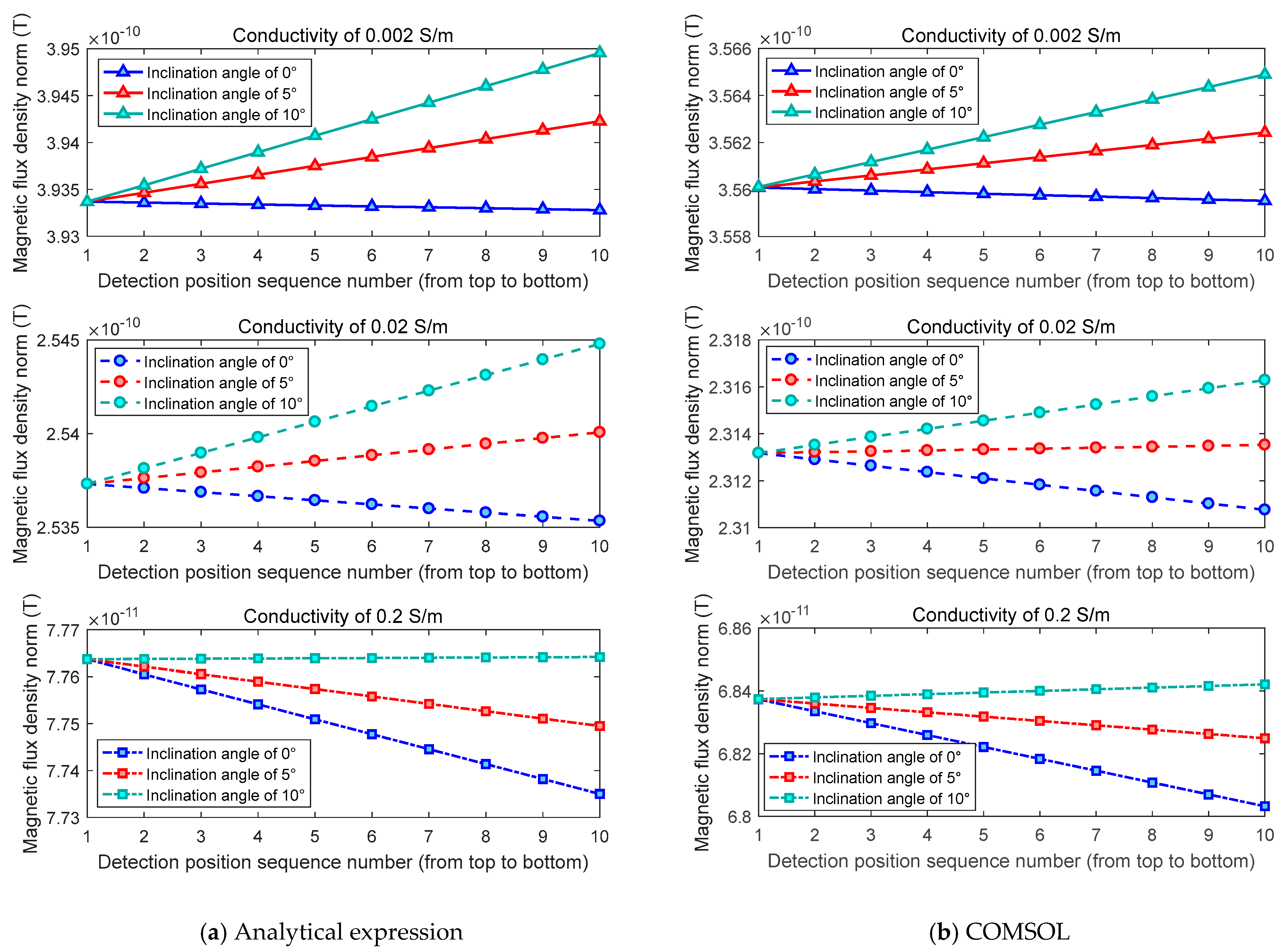
3. Simulation Experiments

To verify the correctness of the analytical expression, a simulation environment was constructed, as shown in Figure 3, and the electromagnetic field distribution was calculated by the analytical expressions derived in Section 2. The multiphysics simulation software COMSOL Multiphysics (version: 6.0) was utilized to simulate the electromagnetic field distribution in the same environment. In Figure 3, the upper layer of the column model is the air domain, whose conductivity is basically 0, and the lower layer is the stratum domain, whose conductivity is 0.02 S/m. Assume that the accident well is a straight well with a depth of 1000 m, and its casing conductivity is 10⁷ S/m. The wellhead of the relief well and the wellhead of the accident well are separated by 200 m, and the surface electrode is deployed near the wellhead of the relief well. Additionally, the excitation electrode is located 500 m below the relief well and 30 m horizontally from the accident well. The simulation parameters are presented in

Table 1. Parameters of the simulation experiment.

Parameters	Value
Position of Downhole Electrode	500 m underground, 30 m away from the target well
Surface Electrode	On the ground, 200 m from the target well
Target Well Length	1000 m
Stratum Conductivity	0.02 S/m
Target Well Conductivity	107 S/m
Current intensity	100 mA
Range of ρ	0–30 m
Range of φ	0–2π
Range of z	−1000–0 m

. Based on the parameters, the COMSOL simulation results and the analytical calculation (run in MATLAB R2023a) results will be compared in terms of different variables.

First, the convergent current on the target well surface was simulated by COMSOL and analytical calculation. The results are illustrated in Figure 4. It can be observed that the variation trends of the convergent current density simulated by the two methods are consistent, and their results are in the same order of magnitude. The convergent current reaches its maximum at the depth position corresponding to the excitation electrode (i.e., near −500 m). As the depth continues to increase, the convergent current gradually decreases. This observation aligns with the basic principle of current injection, thereby validating the rationality of the analytical expression. Additionally, it is noteworthy that since the simplified two-layer model used in the analytical calculation ignores the relief well, which is considered In the COMSOL simulation, the converge current obtained by the analytical calculation is higher than that derived from the COMSOL simulation.

For further comparison, the magnetic field distribution was simulated, and the corresponding placements of the magnetic field detection point are demonstrated in Figure 5. To minimize interference from the primary field generated by the excitation electrode on the effective received signals, three observation lines were set up 100 m below the excitation electrode at inclination angles of 0°, 5°, and 10°, respectively. In each observation line, 10 observation points are distributed uniformly at a spacing of 0.5 m. The observed magnetic field at each point was analyzed with the parameter settings listed in Table 1.

The magnetic fields at the observation positions obtained with the two calculation methods are illustrated in Figure 6. Figure 6a,b show the analytical calculation results and the COMSOL simulation results, respectively. It can be found that the magnetic field results obtained by analytical calculation and COMSOL simulation are also consistent. When the inclination angle of the observation points is 0°, the detected magnetic field gradually decreases from top to bottom; when the inclination angles are 5° and 10°, the detected magnetic field gradually increases from top to bottom due to the change in well spacing. The above variation trend is consistent with the principles of downhole current injection ranging detection.

Keeping other simulation parameters constant, the excitation current was further increased to 300 mA and 500 mA, and analytical calculation and COMSOL-based numerical simulation were employed to obtain the results of converging current density and magnetic field distribution, respectively. Figure 7 shows the results of converging currents around the target well for different excitation levels. It can be observed that the convergent current increases proportionally with the excitation current, both in the analytical and numerical representations. The analytical method provides smoother computational results because it is not affected by the number of mesh grids.

The calculated results of the magnetic field at the corresponding detection locations under different excitations were obtained, as illustrated in Figure 8. It can be found that the magnetic field strength increases with the excitation current, exhibiting an approximately linear growth trend. The above analysis indicates that the computational results of the analytical method align well with the numerical results and demonstrate good adaptability to different excitation cases, thereby confirming the validity of the proposed analytical solution.

Based on the model validity verification, the environmental suitability of the constructed analytical calculation model was further analyzed. With an excitation of 100 mA and other conditions held constant, the stratum conductivity was adjusted to 0.002 S/m, 0.02 S/m, and 0.2 S/m. The converging currents of the target casing and the observed magnetic fields at different locations were then calculated. Figure 9 shows the magnitude of the converging current along the surface of the target casing for different background conductivities. It can be observed that the converging current gradually decreases as the stratum conductivity increases. This phenomenon occurs because as the stratum conductivity increases, the difference between the stratum conductivity and the target casing conductivity becomes smaller, weakening the current convergence ability of the metal casing. Furthermore, when the conductivity changes, the position of the extreme value of the converging current shifts slightly. This indicates that changes in the stratum conductivity also affect the electromagnetic transmission path.

Accordingly, we also calculated the magnetic field for various conductivity cases to analyze the distribution pattern, with the results shown in Figure 10. It is evident that as the stratum conductivity increases, the observed magnetic field at the same location decreases rapidly, which is consistent with the change in converging currents. Notably, the change in stratum conductivity not only affects the magnitude of the magnetic field but also alters its distribution pattern. This observation aligns with the theoretical analysis and confirms that the constructed analytical results are consistent with the results obtained from COMSOL.

4. Conclusions

Considering the advantages and significance of analytical methods in the theoretical study of electromagnetic distribution, this paper derives an analytical solution for electromagnetic signal distribution based on a downhole current-injection ranging environment. First, following the principle of the current injection method, an electromagnetic signal model was constructed, and the corresponding electromagnetic equations were solved. Based on this, the analytical results were compared and analyzed with those of the COMSOL-based numerical simulation method, and highly consistent simulation results were obtained, proving the validity of the proposed analytical solution. Finally, the adaptability and reliability of the proposed analytical solution for the electromagnetic field were demonstrated by simulating the electromagnetic response under different parameter settings.

References

1. Evensen, K.; Sangesland, S.; Johansen, S.E.; Raknes, E.B.; Arntsen, B. Relief well drilling using surface seismic while drilling. In Proceedings of the IADC/SPE Drilling Conference and Exhibition, Fort Worth, TX, USA, 4–6 March 2014. [Google Scholar]
2. Goobie, R.B.; Allen, W.T.; Lasley, B.M.; Corser, K.; Perez, J.P. A guide to relief well trajectory design using multidisciplinary collaborative well planning technology. In Proceedings of the IADC/SPE Drilling Conference and Exhibition, London, UK, 17–19 March 2015. [Google Scholar]
3. Mansouri, V.; Khosravanian, R.; Wood, D.A. Optimizing the separation factor along a directional well trajectory to minimize collision risk. J. Petrol. Explor. Prod. Technol. 2020, 10, 2113–2125. [Google Scholar]
4. Mohamed, A. Anti-collision planning optimization in directional wells. Petrol. Coal 2020, 62, 1144–1152. [Google Scholar]
5. Upchurch, E.; Oskarsen, R.; Chantose, P.; Emilsen, M.; Morry, B. Relief well challenges and solutions for subsea big-bore field developments. SPE Drill. Complet. 2020, 35, 588–597. [Google Scholar]
6. Zhao, W.; Pang, D.; Zhang, Y.; Leng, X. Location selection of deepwater relief wells in south China sea. Petroleum Explor. Dev. 2016, 43, 315–319. [Google Scholar]
7. Poedjono, B.; Nwosu, D.; Martin, A. Wellbore positioning while drilling with LWD measurements. Petrophysics 2019, 60, 450–465. [Google Scholar] [CrossRef]
8. Dou, X.; Liang, H.; Liu, Y. Anticollision method of active magnetic guidance ranging for cluster wells. Math. Probl. Eng. 2018, 2018, 7583425. [Google Scholar] [CrossRef]
9. Diao, B.; Gao, D.; Li, G. Development of static magnetic detection anti-collision system while drilling. In Proceedings of the 2016 International Conference on Artificial Intelligence and Engineering Applications, Hong Kong, China, 12–13 November 2016. [Google Scholar]
10. Poedjono, B.; Alatrach, S.; Martin, A.; Goobie, R.B.; Allen, W.T.; Sweeney, E. Active acoustic ranging to locate two nearby wellbores in deepwater gulf of Mexico. In Proceedings of the SPE Annual Technical Conference and Exhibition, San Antonio, TX, USA, 9–11 October 2017. [Google Scholar]
11. Liu, C.; Dang, J.; Yang, L.; Zhou, Y.; Luo, X.; Dang, B. Space-time pulsed eddy current array for NDT of wellbore casings based on MIMO technique. Proc. IEEE Trans. Instrum. Meas. 2024, 73, 6000112. [Google Scholar]
12. Hanak, F.C.; Estes, R. High speed, continuous single well magnetic ranging. In Proceedings of the IADC/SPE Drilling Conference and Exhibition, London, UK, 17–19 March 2015. [Google Scholar]
13. Hao, X.; Wang, Y.; Dang, B.; Li, F.; Xu, L.; Liu, Z. Research on electromagnetic detection and positioning methods and tools for relief wells. Pet. Drill. Tech. 2021, 49, 75–80. [Google Scholar]
14. Oskarsen, R.T.; Wright, J.W.; Fitterer, D.; Winter, D.; Nekut, A.; Sheckler, J. Rotating magnetic ranging service and single wire guidance tool facilitates in efficient downhole well connections. In Proceedings of the SPE Annual Technical Conference and Exhibition, Amsterdam, The Netherlands, 17–19 March 2009. [Google Scholar]
15. ISCWSA. Well Intercept Sub-Committee Ebook; UHI House: Inverness, UK, 2016; Chapter 3; pp. 25–34. [Google Scholar]
16. Feng, R.; Luo, X.; Yang, L.; Dang, B. Electromagnetic ranging system for rescue wells based on ring MEMS sensors. In Proceedings of the 2024 3rd International Conference on Energy and Electrical Power Systems, ICEEPS, Guangzhou, China, 14–16 July 2024; pp. 1162–1167. [Google Scholar]
17. Diao, B.; Gao, D. A magnet ranging calculation method for steerable drilling in build-up sections of twin parallel horizontal wells. J. Nat. Gas Sci. Eng. 2015, 27, 1702–1709. [Google Scholar] [CrossRef]
18. Wu, Z.; Gao, D.; Diao, B. An investigation of electromagnetic anti-collision real-time measurement for drilling cluster wells. J. Nat. Gas Sci. Eng. 2015, 23, 346–355. [Google Scholar] [CrossRef]
19. Wu, P.; Wei, M. Magnetization influence analysis of the casing and drill pipe in shale gas dual horizontal well Rotating Magnet Ranging System drilling process. Energy Sci. Eng. 2020, 8, 3186–3199. [Google Scholar] [CrossRef]
20. Relief Well Planning & Magnetic Ranging; Halliburton Co.: Houston, TX, USA, 2020; pp. 20–30.
21. Yu, R.; Diao, B.; Gao, D. Optimal selection method of magnetic ranging tools for relief well engineering based on the measurement error of the adjacent well distance. Pet. Drill. Tech. 2021, 49, 118–124. [Google Scholar]
22. Dang, J.; Yang, L.; Zhou, Y.; Dang, B. Sparsity-based nondestructive evaluations of downhole casings technique using the uniform linear array. Appl. Sci. 2024, 14, 6588. [Google Scholar] [CrossRef]
23. Liu, C.; Yang, L.; Zhang, Z.C.; Dang, B. Application of borehole transient electromagnetic system in relief well drilling: A case study. In Proceedings of the 2021 3rd International Conference on Intelligent Control, Measurement and Signal Processing and Intelligent Oil Field (ICMSP), Xi’an, China, 23–25 July 2021. [Google Scholar]
24. Yang, L.; Dang, B.; Liu, C.; Xu, L.; Ren, Z.; Dang, R. Borehole transient electromagnetic array based relative attitude deteation for relief well drilling. In Proceedings of the 2021 3rd International Conference on Intelligent Control, Measurement and Signal Processing and Intelligent Oil Field (ICMSP), Xi’an, China, 27–29 December 2019. [Google Scholar]
25. Peng, H.; Zhao, Y.; Sun, X.; Nie, Z. Numerical investigation of active magnetic ranging method for relief well projects. In Proceedings of the 2021 IEEE International Geoscience and Remote Sensing Symposium IGARSS, Brussels, Belgium, 11–16 July 2021. [Google Scholar]
26. Zhang, S.; Diao, B.; Gao, D. Numerical simulation and sensitivity analysis of accurate ranging of adjacent wells while drilling. J. Pet. Sci. Eng. 2020, 195, 107536. [Google Scholar] [CrossRef]
27. Dang, J.; Yang, L.; Qin, C.; Zhao, Q.; Ji, X.; Guo, C.; Dang, B. Accurate ranging of adjacent well using compressive sensing-based current injection with a uniform sensor array. Geoenergy Sci. Eng. 2024, 233, 212468. [Google Scholar]
28. Wu, Z.; Fan, Y.; Wang, J.; Zhang, R.; Liu, Q.H. Application of 2.5-D finite difference method in logging-while-drilling electromagnetic measurements for complex scenarios. IEEE Geosci. Remote Sens. Lett. 2020, 17, 577–581. [Google Scholar]
29. Wu, S.; Zhao, K.; Yang, S.; Hong, D.; Liu, Q.H. Electromagnetic fields in full-parameter uniaxial anisotropic planar stratified media. IEEE Trans. Antennas Propag. 2024, 72, 2564–2577. [Google Scholar]
30. Wang, X.; Shen, J.; Su, B. 3-D Crosswell electromagnetic inversion based on general measures. IEEE Trans. Geosci. Remote Sens. 2021, 59, 9783–9795. [Google Scholar]
31. Blowout and Well Control Handbook, 2nd ed.; GSM Co.: Amarillo, TX, USA, 2017; pp. 303–336.
32. Dang, J.; Zhao, Q.; Guo, C.; Li, J.; Zhang, L.; Tang, T.; Dang, B.; Yang, L.; Liu, C. Long-Distance Crosswell EM Logging of Copper Ore Using Borehole-Surface Current Injection in Slim Holes. IEEE J. Sel. Top. Appl. Earth Observ. Remote Sens. 2022, 15, 5559–5569. [Google Scholar] [CrossRef]
33. Xu, J. Electromagnetic Field and Electromagnetic Wave in Layered Media; Petroleum Industry: Beijing, China, 1997; pp. 1–244. [Google Scholar]
34. Werner, W. Hamilton-Operator im elektromagnetischen Feld. In Hamiltonsche Mechanik und Quantenmechanik; Springer: Berlin/Heidelberg, Germany, 2023; pp. 439–440. [Google Scholar]
Figure 1. Schematic diagram of current injection ranging in relief well.
Applsci 15 03741 g001
Figure 2. Cylindrical two-layer signal model for current injection system.
Applsci 15 03741 g002
Figure 3. The simulation environment of downhole current injection ranging built by COMSOL.
Applsci 15 03741 g003
Figure 4. Convergent current simulation results.
Applsci 15 03741 g004
Figure 5. Schematic diagram of magnetic field detection point placement.
Applsci 15 03741 g005
Figure 6. Magnetic field simulation results.
Applsci 15 03741 g006
Figure 7. Simulation results of convergent current with different magnitude of excitation current.
Applsci 15 03741 g007
Figure 8. Simulation results of magnetic field with different excitation currents.
Applsci 15 03741 g008
Figure 9. Effect of stratum conductivity on converging currents.
Applsci 15 03741 g009
Figure 10. Effect of stratum conductivity on magnetic fields.
Applsci 15 03741 g010