Abstract
Conventional design methodologies for Frequency Selective Surfaces (FSSs) are often plagued by challenges such as difficulties in determining unit cell structures, a plethora of optimization parameters, and substantial computational demands. In response, researchers have developed deep learning-based approaches for FSS design, highlighting their advantages in terms of high efficiency and low resource consumption. However, these methods are typically confined to designing FSSs within the spectral ranges defined by their datasets, significantly limiting their applicability. This paper systematically analyzes the impact of material and geometric parameters of FSSs on their spectral characteristics, thereby establishing a theoretical foundation for the cross-band transfer learning capability of neural networks. Building on this foundation, we utilized COMSOL (Version 6.0) and MATLAB (Version R2021b) co-simulations to recollect 6000 sets of FSS data in the millimeter-wave band. Using only 23.1% of the data volume, we achieved training results comparable to those obtained with the full dataset in a significantly shorter time frame, with a mean absolute error of 0.07 on the test set. This demonstrates the feasibility of transfer learning and successfully implements cross-band transfer learning of convolutional neural networks from the terahertz band to the millimeter-wave band. The findings of this study provide valuable insights for the integration of deep learning with FSSs, enhancing data utilization efficiency, and further advancing the development of efficient, concise, and universal FSS design methodologies. This advancement extends the scope from solving specific problems to addressing a broader class of issues.
1. Introduction
The frequency range of a terahertz wave is 0.1~10 THz between infrared and micro-wave, with its low energy, strong penetration, spectral information, and other characteristics. It has a wide range of applications in 6G communication [1], food safety [2,3], and biomedicine [4,5,6]. Frequency Selective Surfaces (FSSs), a two-dimensional planar structure of metamaterials, can regulate terahertz amplitude, phase, polarization, and other covariates flexibly and diversely, which provides a brand new platform for the design of miniaturized, high-performance terahertz micro- and nano-optical devices [7,8,9]. The design of FSSs is faced with difficulties including numerous unit structures, parameter complexity, and time-consuming optimization. A simple, efficient, and unified method to complete the design of various FSSs is urgently needed. It is very important for FSSs to move from simulation to engineering.
To address the challenge exposed by the diversity of unit cell structures, researchers have adopted a discretization approach for the periodic structural elements of Frequency Selective Surfaces (FSSs). By integrating full-wave simulation methods with optimization algorithms such as genetic algorithms (GAs) and particle swarm optimization (PSO), intelligent FSS design has been achieved [10,11,12,13], effectively eliminating reliance on empirical expertise. However, this methodology exhibits a notable drawback: the iterative optimization process necessitates repeated calculations of FSS spectral characteristics, resulting in substantial computational time and resource consumption.
With the rapid advancement of artificial intelligence, researchers have begun to explore the use of neural networks as alternatives to traditional analytical methods, numerical techniques, and full-wave simulation software [14,15,16,17,18,19]. Leveraging the framework and principles of deep learning, once the neural network is trained, the spectral characteristics of Frequency Selective Surfaces (FSSs) can be directly obtained by inputting parameters such as discrete encodings of the FSS structure [20]. This approach has demonstrated an efficiency improvement of several orders of magnitude in the simulation process compared to conventional methods. In recent years, scholars both domestically and internationally have paid significant attention to research in this area [21,22,23]. In 2019, Qiu Tianshuo and colleagues from the Chinese Air Force Engineering Research Institute employed deep learning techniques to accurately predict discrete coding metasurface structures and design a tri-band absorber [24]. Their study utilized a training set comprising 70,000 data samples and a validation set of 10,000 data samples. Similarly, Y. Li and collaborators from the Harbin Institute of Technology implemented a multifunctional transmit array metasurface design capable of frequency reuse and polarization reuse by integrating neural networks with genetic algorithms. Their approach involved a training set of 36,000 data samples and a validation set of 4000 data samples [25].
Deep learning-based FSS design methods, while significantly enhancing efficiency during the design phase, still require substantial time and resources for data collection. Consequently, scholars have begun exploring transfer learning to reduce data requirements and improve data utilization efficiency [26,27]. Dong Xu [17] realized the transfer learning of FPN from rectangular meta-atoms to elliptical meta-atoms, which was used to predict real part spectra and imaginary part spectra in the range of 100~300 THz. Compared with the training process of the two neural networks, the former without transfer learning had a data size of 27,000, and the latter with transfer learning had a data size of 4500, and the training time was reduced from 4 h to 20 min, and the test error was reduced from 0.00076 to 0.00067. Ruichao Zhu et al. [18] used Goog-LeNet-Inception-V3 to predict the phase of a 28 × 8 meta-atom with an accuracy of about 90%, realizing transfer learning from the field of image processing to the field of metasurface prediction. Zhixiang Fan et al. [19] achieved transfer learning from cheap and simple source metasurface data (5 × 5) to intensive and complex data (20 × 20) by an encoder–decoder network. This transfer can speed up the metasurface design process and save target data. Previous studies have achieved the efficient design of FSSs within a defined frequency range, which is typically limited by the dataset. If an FSS needs to be designed in other frequency ranges, it becomes necessary to collect data and retrain the neural network again by the usual approach. However, collecting data is the most time-consuming and resource-intensive step, and how to improve data utilization efficiency and save computing resources remains the difficulty in developing FSS design methods based on deep learning.
In this paper, the influence of FSS parameters on its spectral characteristics is analyzed in detail. The theoretical basis for transferable learning in the FSS design method, combining deep learning with intelligent algorithms, is clarified. More convolutional neural networks are implemented for transfer learning from terahertz to millimeter-wave bands. This research provides a reliable reference for the cross-fusion of deep learning and FSSs. FSS design has been further developed in an efficient and universal way.
2. FSS Structure Design and Spectral Characterization Analysis
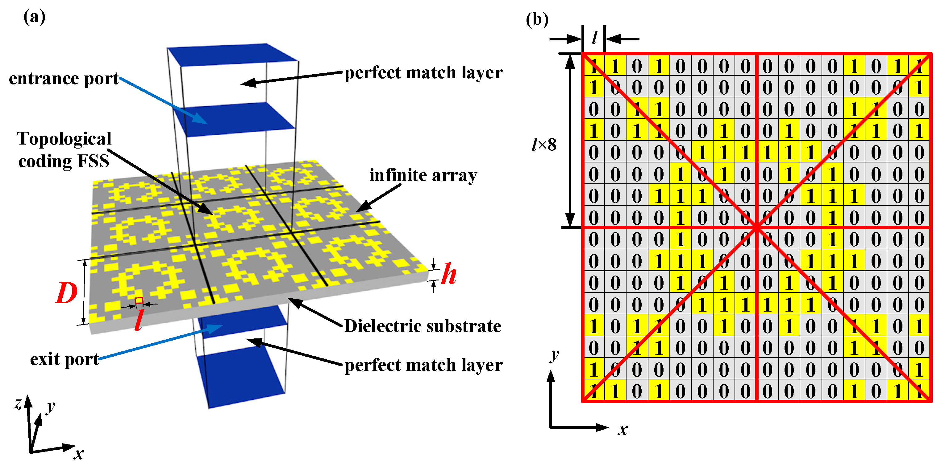
The FSS simulation structure is shown in Figure 1. Figure 1a shows the three-dimensional simulation schematic of the FSS with the following features: the substrate was of high-resistance silicon, in the terahertz band its refractive index was , the absorption can be ignored [28], and the thickness of the substrate was 5 μm. The external medium was air and the absorption can be ignored [28]. The surface of the dielectric substrate was covered with a thin layer of gold, and its conductivity was , and its thickness was . The cycle length of the FSS was .
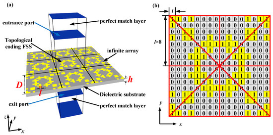
Figure 1.
Schematic diagram of the FSS simulation structure. (a) 3D simulation structure and (b) FSS topological code.
The corresponding coding unit structure is shown in Figure 1b. The period unit is discretized into small squares with a side lengths of , in which the number “1” denotes the thin gold layer and the number “0” denotes the substrate. Therefore, the FSS was composed of 16 by 16 “0/1” matrices with one-to-one correspondence.
Considering the polarization stability of FSSs, all FSSs were set as rotationally symmetric structures. Figure 1b demonstrates the four symmetry axes of the FSS, which reduced the degrees of freedom of the FSSs from 216×16 to 236. It reduced the difficulty of FSS optimization design greatly.
Following the completion of the FSS symmetric structure model, the simulation was conducted utilizing COMSOL. The boundary condition was designated as the Floquet periodic condition, with a simulation frequency range of 0.5–3 THz and a step size of 0.02 THz, consequently yielding a total of 126 frequency points. The electromagnetic properties of the FSS were characterized in this study by means of the total transmittance, total reflectance, and total absorptance, in order to investigate its transmission and reflection characteristics. The spectra of the “ring-shaped” encoded FSS under TE and TM conditions are shown in Figure 2a,b, respectively. It can be observed that the two spectra are nearly identical. A similar conclusion can be drawn from the calculation results of other randomly encoded FSSs that satisfy rotational symmetry, thereby verifying the polarization stability of the rotationally symmetric structure.
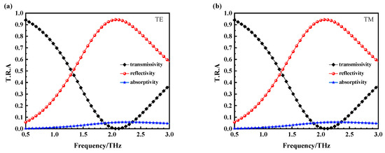
Figure 2.
Comparison of the polarization of the “circular” encoded FSS. (a) TE; (b) TM.
The dataset serves as the cornerstone of deep learning, where both the quantity and quality of data directly influence the training efficacy of neural networks. The dataset in this study comprised two components: the binary “0/1” matrices corresponding to the Frequency Selective Surface (FSS) configurations and their associated spectral responses. To optimize data generation efficiency, 26,000 unique pairwise-distinct “0/1” matrices were randomly generated. An automated workflow was implemented using MATLAB (Version R2021b) to control COMSOL (Version 6.0) Multiphysics, sequentially constructing FSS models for each matrix, performing electromagnetic simulations, and exporting the computed spectral responses to MATLAB for post-processing and archival storage.
Due to the large amount of data required, and in order to save computation time, “transition boundary conditions” were used instead of thin metal layers to avoid mesh partitioning. Additionally, mesh partitioning settings were optimized to minimize the number of elements and accelerate the computation speed.
Table 1 provides a comparative analysis of two meshing strategies in terms of element count and computational time. The physics-controlled meshing, an automated COMSOL algorithm that determines element size based on the highest frequency in the operational band, delivered higher numerical accuracy. In contrast, the user-defined meshing allowed researchers to manually specify element dimensions tailored to specific simulation requirements.

Table 1.
Comparison of meshing element counts.
Figure 3 compares the computational results of the same frequency-selective surface (FSS) using two meshing strategies, demonstrating close agreement between the two approaches. In Figure 3, the dashed line represents the spectral curve obtained with the default physics-controlled meshing, while the solid line corresponds to the user-defined meshing, achieving a 56.7% reduction in computational time. The maximum and mean absolute errors (MAE) for key performance metrics were quantified as follows: (1) transmittance: maximum error = 0.0445, MAE = 0.0193; (2) reflectance: maximum error = 0.2425, MAE = 0.0291; and (3) absorptance: maximum error = 0.1265, MAE = 0.0173.
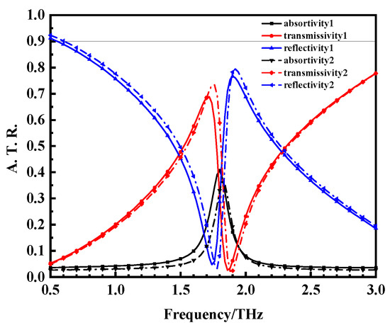
Figure 3.
Comparison of simulation results of different mesh profiles.
The elevated reflectance error at 1.86 THz was attributed to sharp fluctuations in transmittance near the FSS resonance frequency, where field gradients challenge mesh resolution. Despite this localized discrepancy, the low MAE for reflectance (0.0291) confirmed that the slight resonance frequency shift caused by the reduced mesh density negligibly impacted the overall spectral characteristics of the FSS. This validates the applicability of the user-defined meshing strategy for large-scale dataset generation while significantly accelerating simulations.
Further optimization was achieved by replacing the default MUMPS solver with the PARDISO solver, explicitly designed for parallel computing. This adjustment reduced the per-simulation computation time to 2 min and 22 s, enhancing workflow efficiency for the 26,000-sample dataset.
The FSS parameters were mainly categorized into two types: geometrical parameters and material parameters. Geometrical parameters include the period length D of the FSS, the thickness h of the substrate, and the thickness h0 of the metal film layer. Material parameters include the metal conductivity and the refractive index of the substrate. For the convenience of later discussion, all FSSs in this paper used the encoding as shown in Figure 1b, unless otherwise stated.
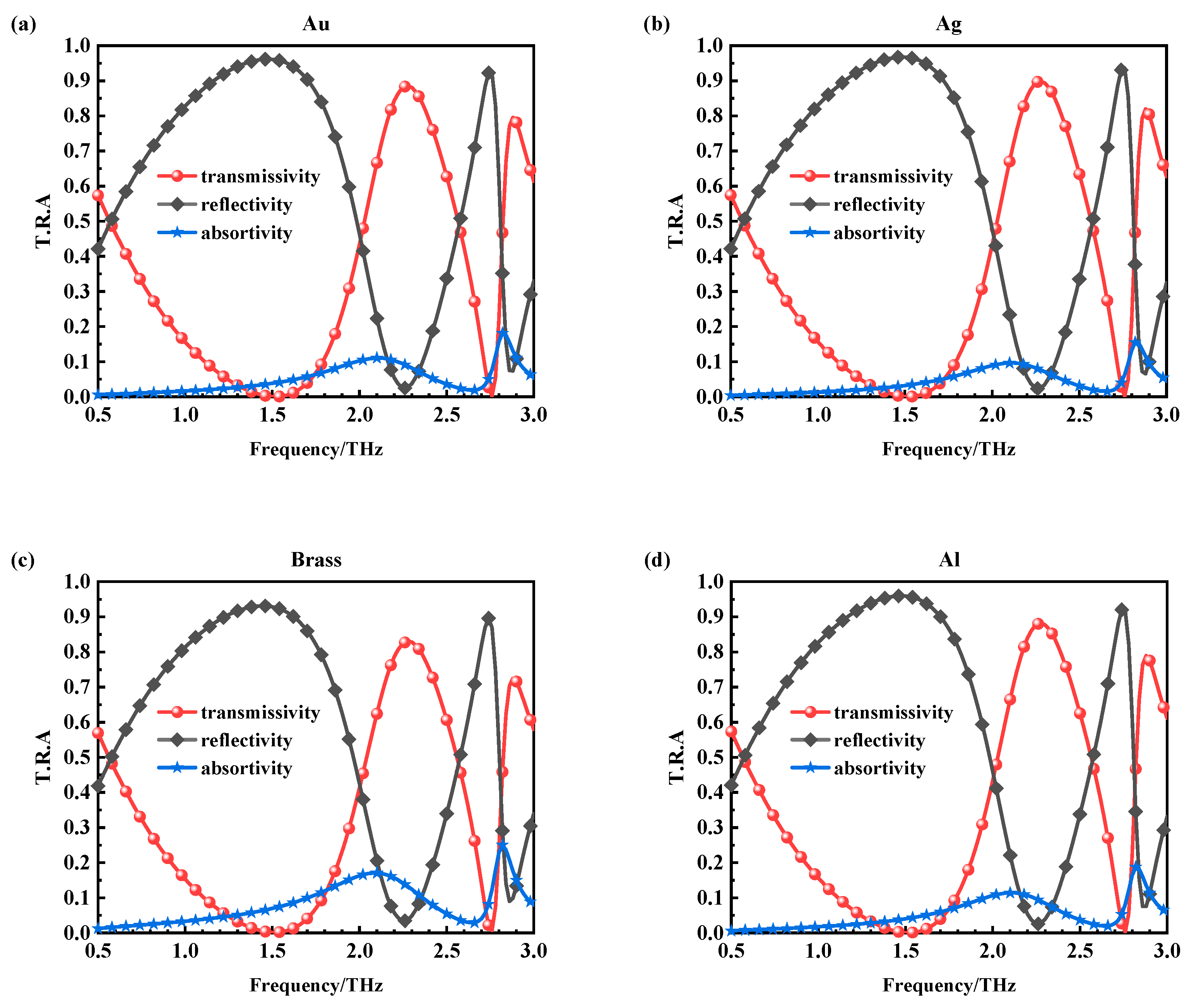
Figure 4 demonstrates the spectral properties of different metals of the same FSS surface model. Figure 4a–d are gold, silver, brass, and aluminum, respectively, whose conductivities are shown in Table 2. It can be found that the spectral properties were almost identical. This phenomenon is determined by the interaction between light and metal. The calculation of the skin depth is as follows:
where is skinning depth of the metal, is the frequency of electromagnetic wave, is magnetic permeability of the metal, for non-magnetic media take , and is conductivity of the metal.
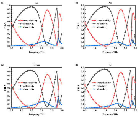
Figure 4.
Spectral curves of different metal coatings for the same FSS model. (a) Gold, (b) silver, (c) brass, and (d) aluminum.
Table 2.
Conductivity and its skinning depth for various common metals.
Table 2 gives the common types of metal conductivity, the simplified skinning depth formula, and its skinning depth at 1 THz. It can be seen that the skinning depth at 1 THz of each type of metal was less than 200 nm. When the thickness of the metal was 200 nm, the effect of different metal types on the spectral characteristics of the FSS was relatively small and could be ignored.
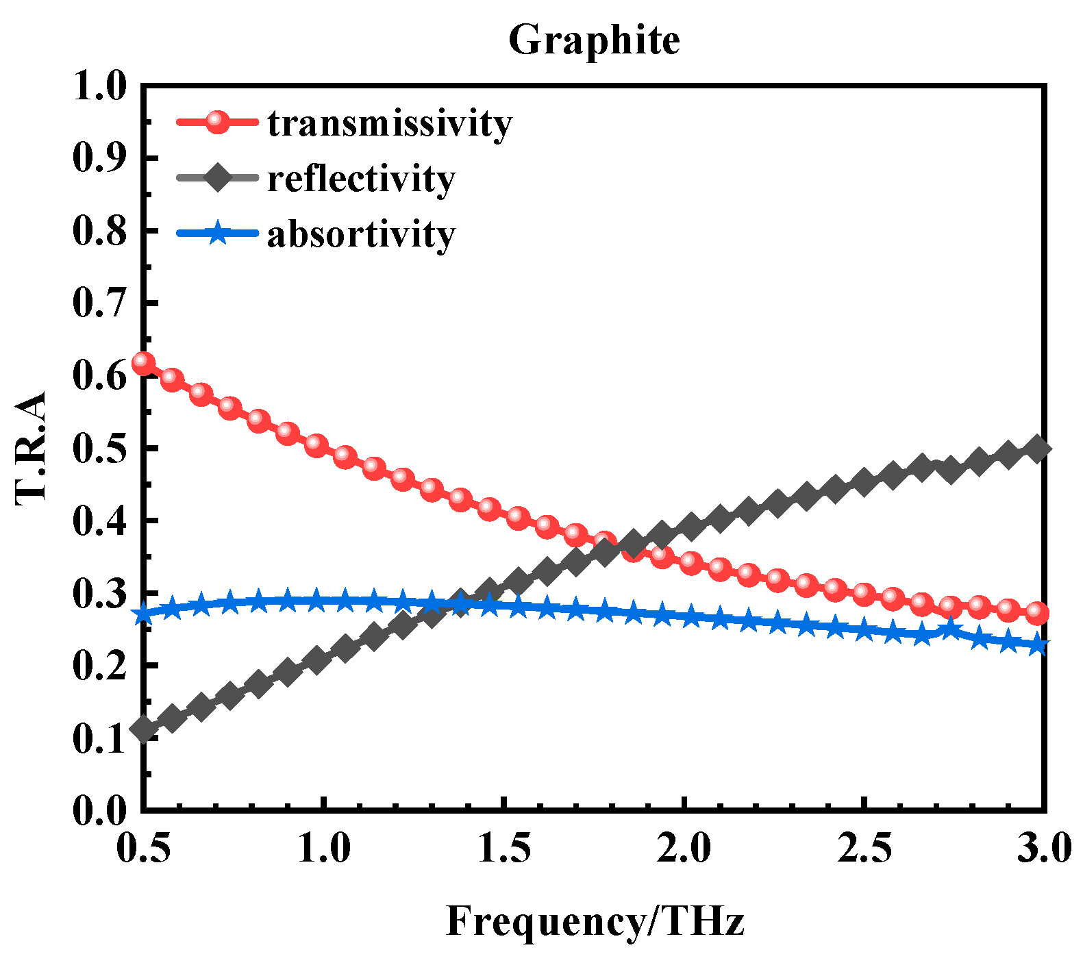
Figure 5 shows the spectral characteristics of the FSS when the surface coating was changed to graphite. Due to the difference of two orders of magnitude between the electrical conductivity of graphite and that of the metal, the skinning depth reached 1600 nm at the incident electromagnetic wave frequency of 1 THz, which is much larger than that of the coating thickness of 200 nm, resulting in an obvious change in the spectral curve.
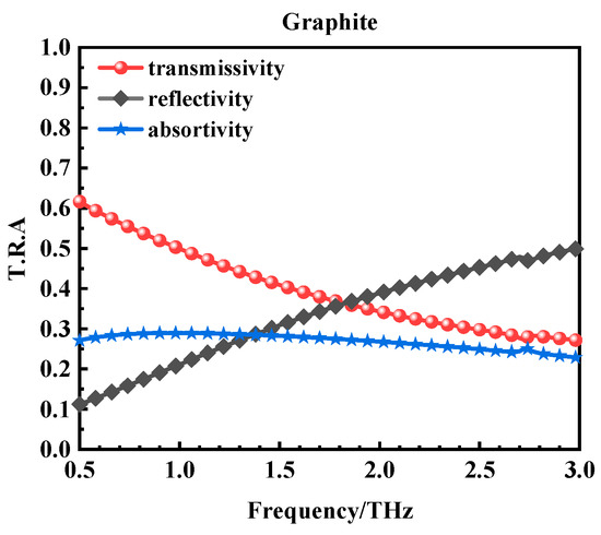
Figure 5.
Spectral profile of graphite coating with the same FSS model.
Figure 6 shows that spectral properties of different thicknesses of the same substrate with the same FSS model. The thickness of the substrate in Figure 6a is , and the thickness of the substrate in Figure 6b is . The metal type of both models was Au and the type of substrate was high-resistance silicon. They are compared with Figure 2a. The high transmissivity resonance points of the different substrate thicknesses are shown in Table 3. The trend is that as the substrate thickness increases, the resonant frequency of FSS shifts towards lower frequencies and the overall trend is similar, but the transmittance decreases overall.
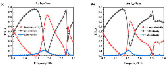
Figure 6.
Spectral curves of different thicknesses of the same substrate with the same FSS model. (a) h0 = 5 μm (b) h0 = 8 μm.
Table 3.
Comparison of resonance points with different substrate thicknesses for the same FSS model.
The resonant frequency of the FSS shifted when a substrate of infinite thickness was loaded unilaterally, which is given as follows:
In the above analysis, either the increase in the relative permittivity of the substrate or the increase in the thickness of the substrate was equivalent to the increase in the equivalent permittivity , which led to the shift of the resonant frequency of the FSS to the lower frequency. The simulation results are in good agreement with the theoretical results.
As a subwavelength structure, the period length of FSS should be comparable to the wavelength corresponding to the highest frequency of the incident electromagnetic wave. When the wavelength was much smaller than the period length, the incident electromagnetic wave exhibited a geometrical optics-like property. When the wavelength was longer than the period length, it could not control electromagnetic waves due to the drastic changes in its transmittance spectrum.
Figure 6 shows the comparison results of the spectral properties of the FSS for the same FSS model by expanding its period length by a factor of 100 accordingly when the maximum frequency of the incident electromagnetic wave was reduced by a factor of 100. That is, when the corresponding wavelength was kept equal to it, the comparison results of the frequency spectrum characteristics of FSS. The comparison of the parameters of the cross-band FSS model is shown in Table 4 below.
Table 4.
Comparison of cross-band FSS model parameters.
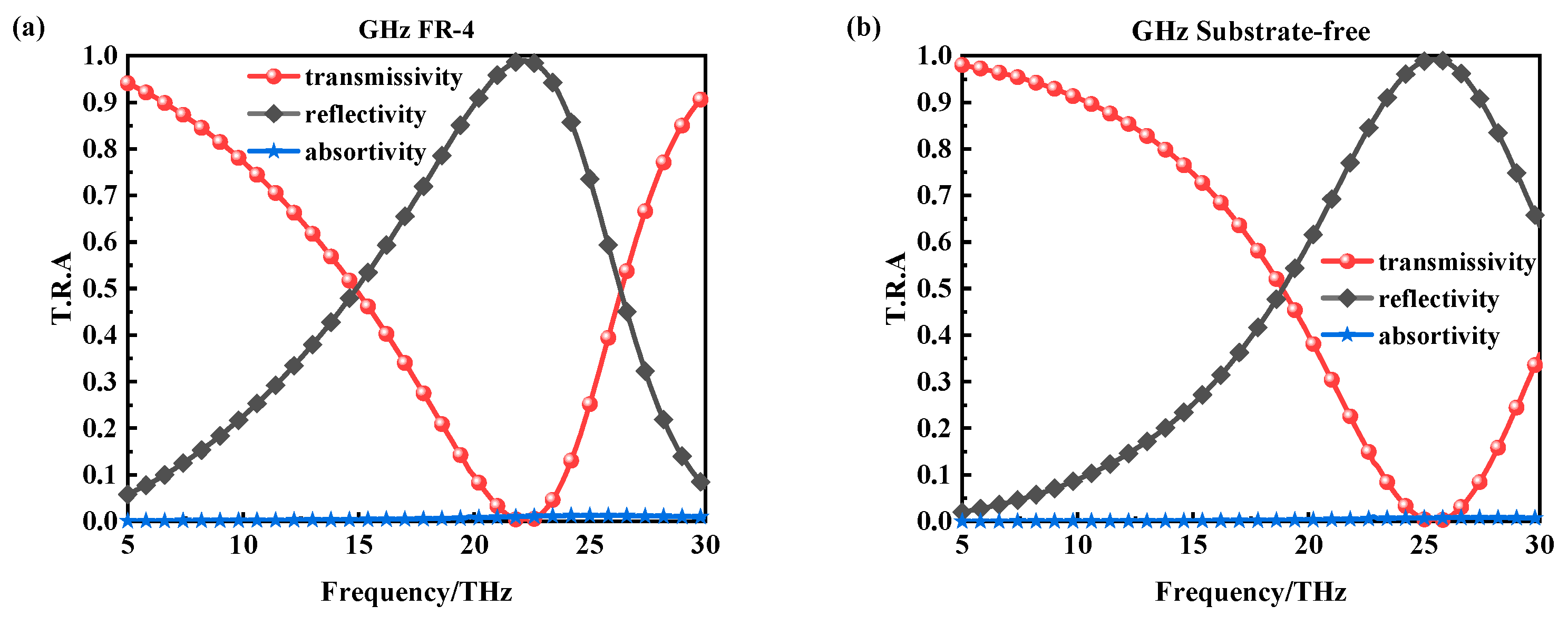
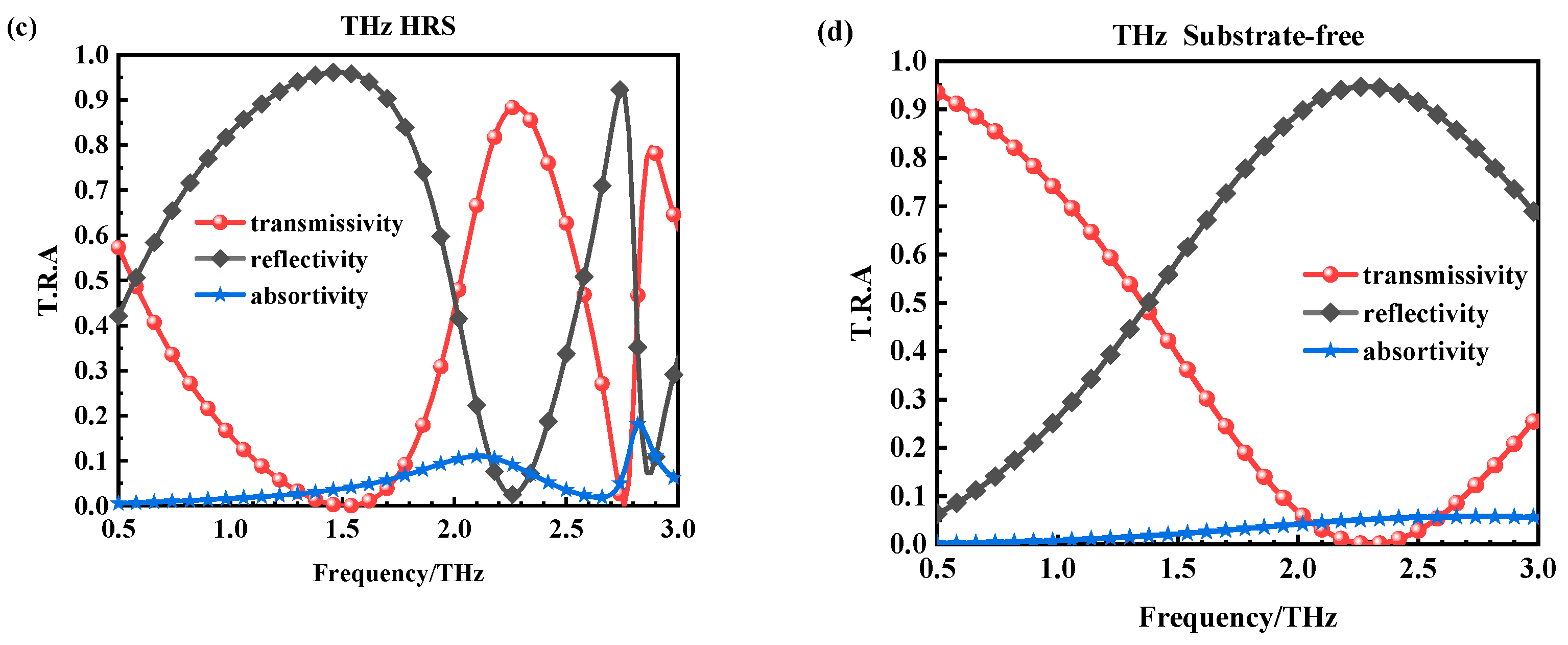
Comparing Figure 7a with Figure 7c, it can be found that the spectral curves of the two are very different due to the differences in the substrate thickness and relative dielectric constant. However, if the effect of substrate was excluded and the substrate thickness of both FSS models was set to 0, the spectral curves of the two would trend as-shown in Figure 7b with Figure 7d, respectively. It can be seen that although their spectral curves were not exactly the same, the spectral curves of the two had a similarity in the trend. A similar conclusion can be obtained by changing the coding of the FSS. This means that FSSs with a certain geometry can have similar spectral characteristics in different electromagnetic wave frequency ranges by scaling their geometrical size.
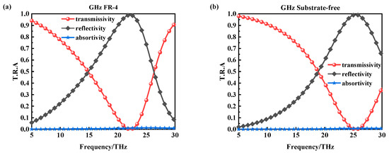

Figure 7.
Cross-band comparison for the same FSS model. (a) GHz band Rogers5880, (b) GHz band without substrate, (c) THz band High resistance silicon, and (d) THz band without substrate.
According to the above analysis, the influence law between the parameters of FSS and its spectral characteristics can be summarized as follows:
- When the metal thickness of the FSS was greater than its skin depth, the spectral characteristics of FSS with different metal types and thicknesses were similar;
- Different thicknesses of substrates affected their equivalent dielectric constants, resulting in a shift in the resonant frequency of the FSS;
- When the period length of FSS was scaled at the same time and the highest frequency of incident electromagnetic wave was the same multiple, the spectrum curves of FSS before and after scaling were similar for pure metal FSS with the same shape.
3. Cross-Band Transfer Learning for FSS
The conclusions drawn in the previous section can be used to realize cross-band transfer learning for FSS. The millimeter-band FSS model determined by Table 4 was adopted, i.e., the width of the small square grid encoded by the FSS was enlarged by 100 times from 5 um to 0.5 mm. The number of small squares in each cycle unit was kept 16 × 16. The corresponding frequency of the incident electromagnetic wave was narrowed by 100 times from 0.5~3 THz to 5~30 GHz. Its corresponding wavelength was enlarged by 100 times, keeping the cycle length comparable to that of the FSS. In addition, the substrate high-resistance silicon was changed to FR-4 commonly used in the microwave band, which had a relative dielectric constant of 4.3 and a substrate thickness of 1 mm.
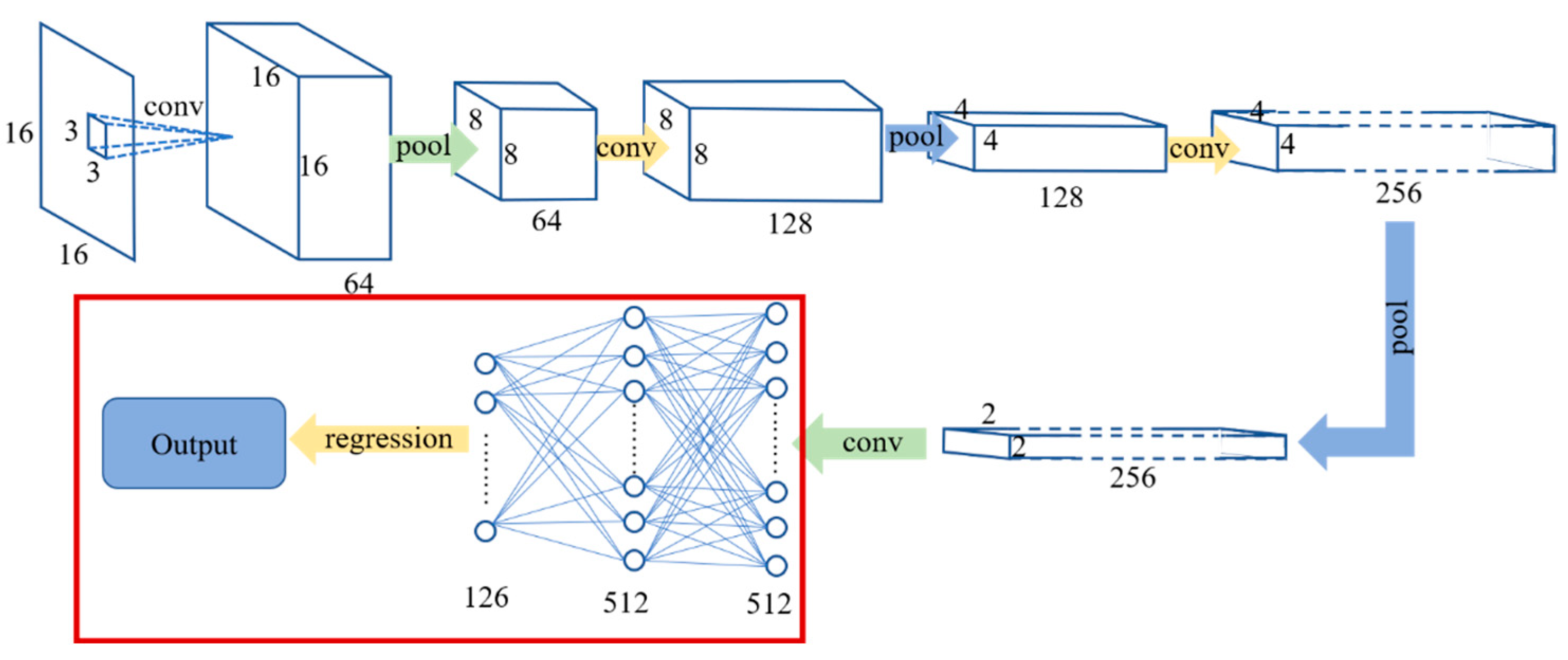
Using a combination of MATLAB and COMSOL simulations, 26,000 sets of data in the THz band and 6000 sets were collected in the microwave band. The structure of the convolutional neural network is shown in Figure 8. The input “image” was a 16 × 16 “0/1” matrix. The output was a 1 × 126 predicted spectral curve. The structure was mainly composed of two parts. They were the “convolution-pooling” part, which was used to extract image features, and the “fully connected” part, which was used to output the spectral curve. The loss function MSE is [29]:
where is the CNN prediction result, is the COMSOL simulation result, and N is the number of frequency points.
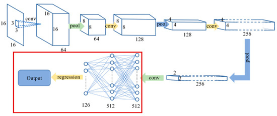
Figure 8.
Schematic of Convolutional Neural Network Transfer Learning.
The convolutional neural network in the THz band trained the neural network from random initialization, while the CNN in the millimeter band trained the neural network using transfer learning on the basis of the former. According to the previous analysis, the same FSS coding matrix had similar spectral properties in different electromagnetic wave bands when certain conditions were satisfied. When transfer learning is used to train the neural network, the convolutional part used to extract the coding features should be frozen and the fully connected part should be retrained. The other training details were exactly the same for both.
During the training process of the neural network, the Adam adaptive gradient de-scent algorithm was used to update the weights. The initial learning rate was set to 0.001. The exponential decay was used to adjust the learning rate, i.e., the learning rate decreased to the original 0.5 every 5 rounds:
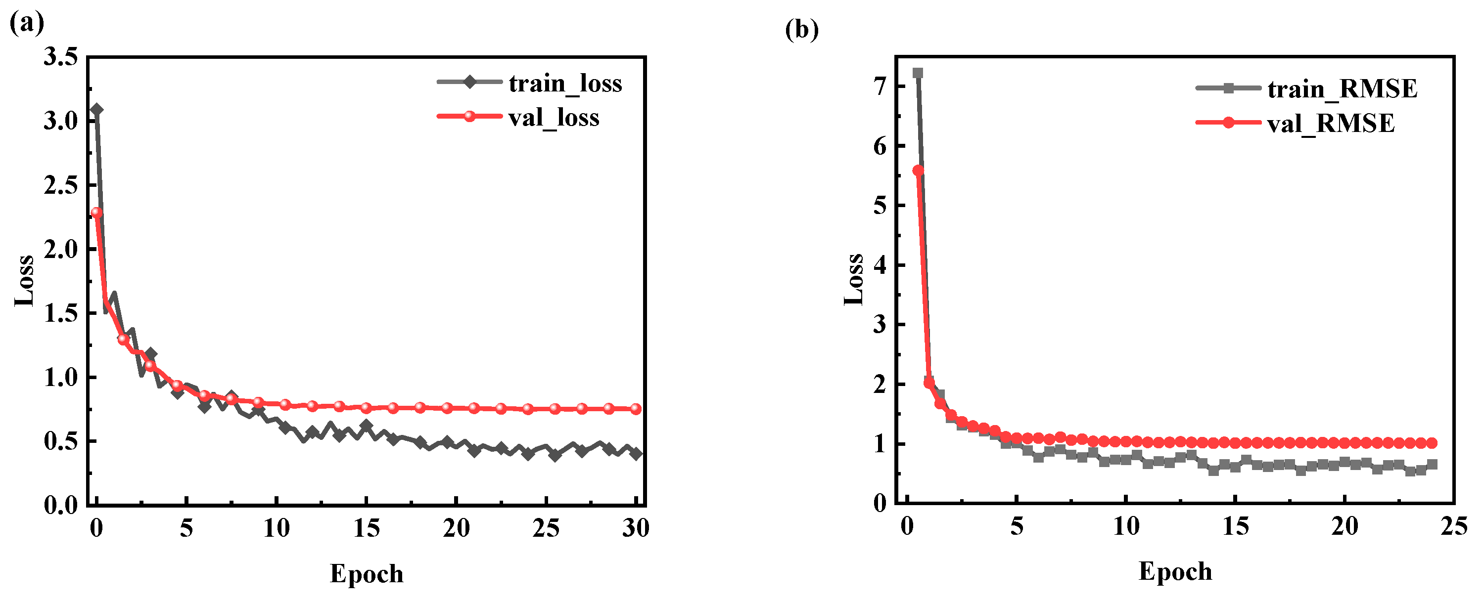
where LearnRate is the learning rate corresponding to each round of training and epoch is the number of rounds of training. A total of 80% of the dataset was the training set and 20% was the test set. The training process is shown in Figure 9. Figure 9a shows the training process of the THz-band CNN. After 20 rounds of training, the error of the test set tends to be stabilized. Total training time was 18 min. Figure 9b is the training process of the millimeter-band CNN. Due to the reduction of the data volume, the total training time was only 1.5 min, much lower than the former.
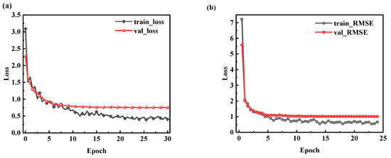
Figure 9.
Illustration of Convolutional Neural Network Training Process. (a) Loss value variation graph; (b) RMSE variation graph.
After the training was completed, two neural networks were validated using their respective test sets and the neural network outputs were compared with the COMSOL simulation results. Their objective evaluation results are shown in Table 5. is the mean absolute error, is the root mean square error, and values range from 0 to 1, which is used to describe the degree of fitting between them. The formulas are as follows [30]:
where is the CNN prediction result, is the COMSOL simulation result, is the average value of the simulation result, and N is the number of frequency points.
Table 5.
Comparison of CNN prediction results for THz and millimeter bands.
The training process is shown in Figure 10. It can be observed that due to the reduced amount of data, the training results quickly reached stability. After training, the objective evaluation metrics were as follows: MAE was 0.0719, RMSE was 0.1267, and R-squared (R2) was 0.8145. Compared to the objective evaluation metrics from training from scratch (MAE of 0.0592, RMSE of 0.1005, and R2 of 0.6692), both MAE and RMSE increased, indicating that the errors had grown and the performance of the neural network had worsened. However, R2 had increased, indicating improved fit, and thus the neural network’s performance appeared better, showing a contradiction. This is because the data used in millimeter-wave transfer learning were a subset of terahertz-wave data, which enhanced the prediction results. In a comprehensive analysis, the performance of the neural network trained with transfer learning should be weaker than that of the network trained from scratch, but transfer learning only used 23.1% of the former’s data, and both methods showed comparable performance. This makes transfer learning an important and meaningful neural network training approach.
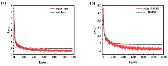
Figure 10.
Transfer Learning Training Process. (a) Loss value variation graph; (b) RMSE variation graph.
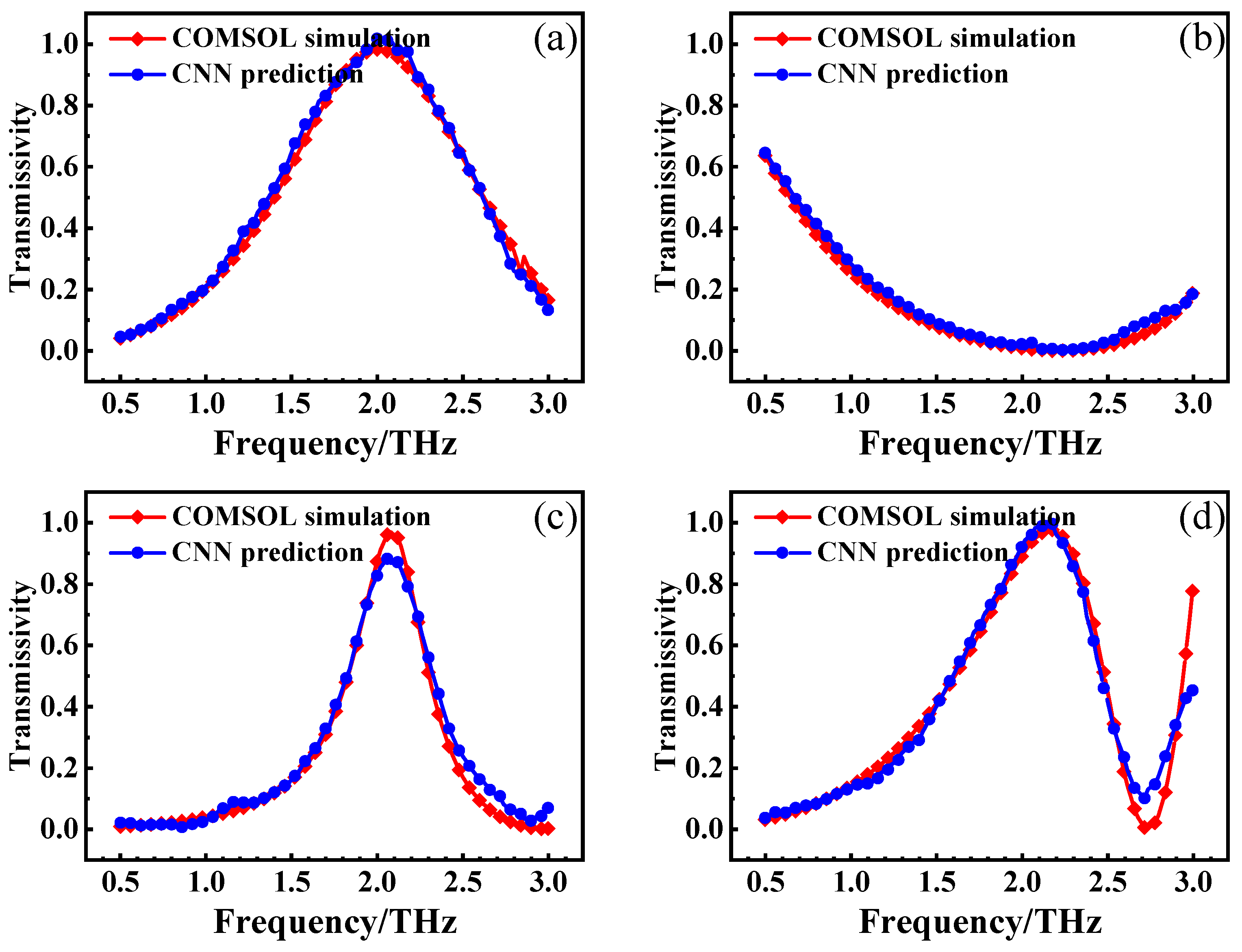
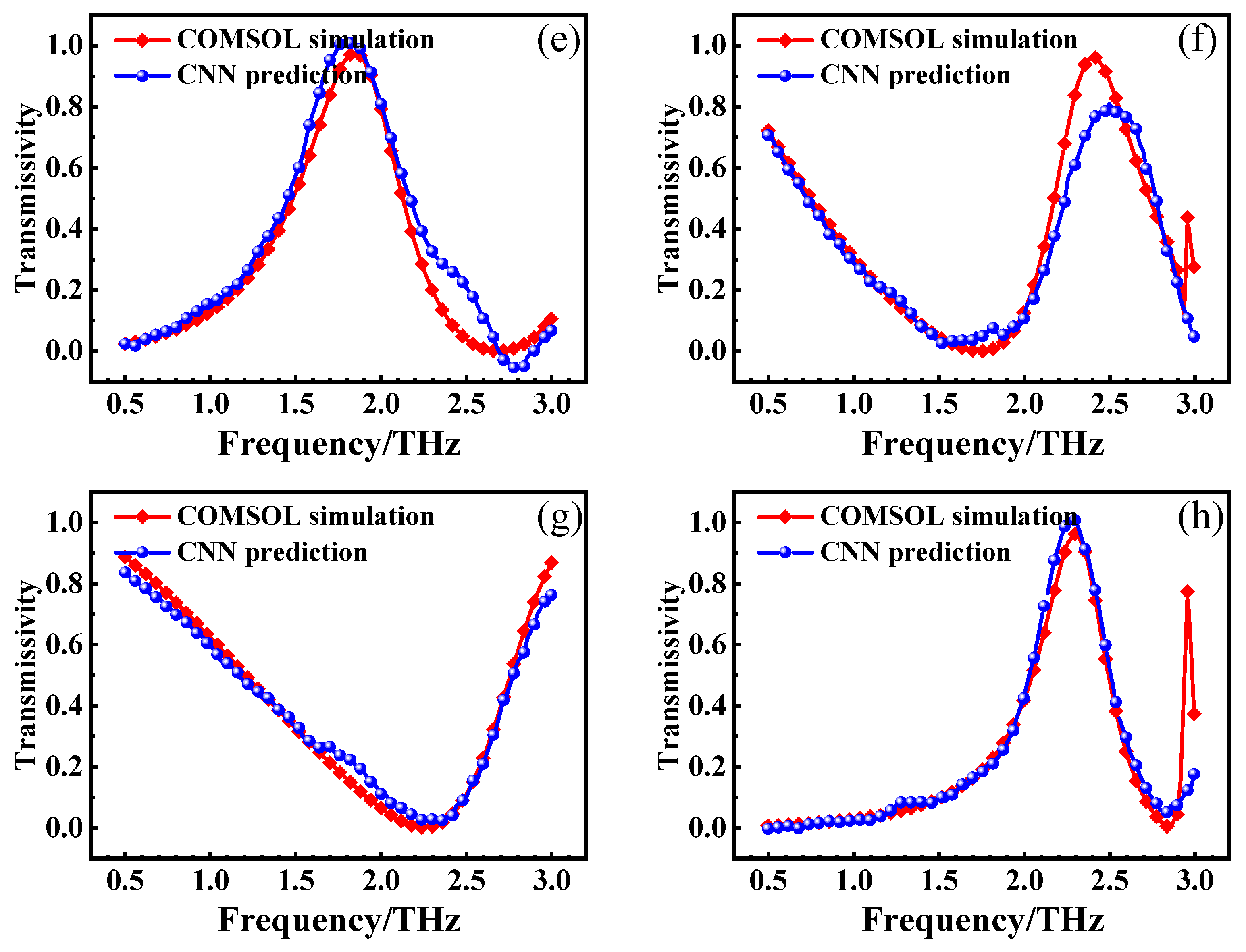
After the training of the transfer learning neural network was completed, some of the results were randomly selected for comparison. The comparison results are shown in Figure 11. It was found that both the training set and the test set had a high degree of fit, which is comparable to the effect of the neural network trained from scratch by the THz CNN.
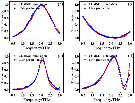
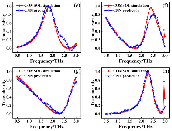
Figure 11.
Comparison of transfer learning neural network results. (a–d) Training set. (e–h) Test set.
After completing the training of the transfer learning neural network, the convolutional neural network and the genetic algorithm can be jointly used to complete the design of various types of typical FSSs in microwave bands. It is worth mentioning that this paper only takes microwave bands as an example to show that this method of transfer learning is feasible in cross-band FSS design. Advantages of concise and efficient deep learning can be further brought out due to the reduction in the amount of original data from 26,000 to 6000 groups, which is a reduction of 76.9%. The method can be applied to other bands where necessary through the same steps to expand the method from solving a specific problem to solving a certain class of problems, greatly expanding the application range of the method.
4. Conclusions
In this paper, the FSS periodic units were coded as 16 × 16 “0/1” rotationally symmetric matrices, each coded unit was guaranteed to have randomness, and 26,000 sets of transmittance and reflectance spectra in the range of 0.5–3 THz were collected as a dataset using the joint simulation of COMSOL and MATLAB. A 19-layer convolutional neural network was used to realize the FSS spectrum prediction, the average absolute error of the test set was as low as 0.06 and the single prediction time was as low as 0.09 s. In addition, the effects of various geometrical and material parameters of the FSS on the spectral characteristics of the FSS were analyzed in detail and conclusions were drawn as follows: (1) when the metal thickness of the FSS is larger than its skinning depth, the spectral characteristics of FSSs with different metal types and thicknesses are similar; (2) the resonance frequency of the FSS was shifted by equivalent dielectric constant with different thicknesses of substrates; and (3) when the period length of the FSS was scaled at the same time and the highest frequency of incident, and the electromagnetic wave was the same multiple, the spectrum curves of FSS before and after scaling were similar for pure metal FSS with the same shape.
On this basis, 6000 sets of millimeter-band FSS data were re-collected using COMSOL and MATLAB joint simulation, the already trained convolutional neural network in the THz band was used to transfer learning the data, which can achieve a comparable training effect with the former one after 1 min 14 s training time, and the average absolute error of the test set was 0.07. This study innovatively extended the cross-fusion of deep learning and FSSs from solving a specific problem to solving a certain class of problems.
The dataset in this study was initially designed with a focus on universality, endowing the Frequency Selective Surface (FSS) codes with two fundamental characteristics: element-wise stochasticity and global rotational symmetry. These intrinsic properties impose significant challenges for neural networks in inverse design tasks, requiring simultaneous generation of randomly distributed unit elements while maintaining strict rotational symmetry at the macro level. Experimental results demonstrate that conventional convolutional neural networks (CNNs) fail to accomplish this dual-constrained generation task. Although transformer-based architectures show potential in producing qualified FSS codes that satisfy both geometric requirements, the spectral response curves of generated patterns still exhibit non-negligible deviations from the original designs, indicating the necessity for further accuracy improvements. Future work will focus on three critical directions: expanding the training dataset scale; optimizing algorithm architectures and modelling addresses that influence geometric and material parameters on spectral responses, which is fundamental to the design of FSS; and a method to improve the robustness of the numerical simulation of FSS by introducing error correction strategies based on physical models [31].
Author Contributions
Conceptualization, L.G. and Z.Y.; methodology, L.G.; formal analysis, P.Z. and X.L.; writing original draft preparation, X.L.; writing—review and editing, Z.Z and L.W. All authors have read and agreed to the published version of the manuscript.
Funding
This research was funded by the Youth Innovation Team of Shaanxi Universities, grant number K20220184; the Key Scientific Research Plan of the Education Department of Shaanxi, grant number 23JY035; and the Natural Science Foundation of Shaanxi Province, grant number 2024JC-YBMS-523.
Institutional Review Board Statement
Not applicable.
Informed Consent Statement
Not applicable.
Data Availability Statement
The data that support the findings of this study are available from the corresponding author L.G. upon reasonable request.
Acknowledgments
The authors sincerely appreciate all financial and technical support.
Conflicts of Interest
The authors declare no conflicts of interest.
References
- Althuwayb, A.A.; Rashid, N.; Elhamrawy, O.I.; Kaaniche, K.; Khan, I.; Byun, Y.-C.; Madsen, D.Ø. Design and Performance Evaluation of a Novel Metamaterial Broadband THz Filter for 6G Applications. Front. Mater. 2023, 10, 1245685. [Google Scholar] [CrossRef]
- Fu, X.; Liu, Y.; Chen, Q.; Fu, Y.; Cui, T.J. Applications of Terahertz Spectroscopy in the Detection and Recognition of Substances. Front. Phys. 2022, 10, 869537. [Google Scholar] [CrossRef]
- Shen, S.; Liu, X.; Shen, Y.; Qu, J.; Pickwell-MacPherson, E.; Wei, X.; Sun, Y. Recent Advances in the Development of Materials for Terahertz Metamaterial Sensing. Adv. Optical Mater. 2022, 10, 2101008. [Google Scholar] [CrossRef]
- Jain, P.; Chhabra, H.; Chauhan, U.; Prakash, K.; Gupta, A.; Soliman, M.S.; Islam, M.S.; Islam, M.T. Machine Learning Assisted Hepta Band THz Metamaterial Absorber for Biomedical Applications. Sci. Rep. 2023, 13, 1792. [Google Scholar] [CrossRef] [PubMed]
- Chen, X.; Lindley-Hatcher, H.; Stantchev, R.I.; Wang, J.; Li, K.; Hernandez Serrano, A.; Taylor, Z.D.; Castro-Camus, E.; Pickwell-MacPherson, E. Terahertz (THz) Biophotonics Technology: Instrumentation, Techniques, and Biomedical Applications. Chem. Phys. Rev. 2022, 3, 011311. [Google Scholar] [CrossRef]
- Park, S.J.; Hong, J.T.; Choi, S.J.; Kim, H.S.; Park, W.K.; Han, S.T.; Park, J.Y.; Lee, S.; Kim, D.S.; Ahn, Y.H. Detection of Microorganisms Using Terahertz Metamaterials. Sci. Rep. 2014, 4, 4988. [Google Scholar] [CrossRef]
- Wang, W.; Sun, K.; Xue, Y.; Lin, J.; Fang, J.; Shi, S.; Zhang, S.; Shi, Y. A Review of Terahertz Metamaterial Sensors and Their Applications. Opt. Commun. 2024, 556, 130266. [Google Scholar] [CrossRef]
- Xing, H.; Fan, J.; Lu, D.; Gao, Z.; Shum, P.P.; Cong, L. Terahertz Metamaterials for Free-Space and On-Chip Applications: From Active Metadevices to Topological Photonic Crystals. Adv. Devices Instrum. 2022, 2022, 9852503. [Google Scholar] [CrossRef]
- Lyu, J.; Huang, L.; Chen, L.; Zhu, Y.; Zhuang, S. Review on the Terahertz Metasensor: From Featureless Refractive Index Sensing to Molecular Identification. Photon. Res. 2024, 12, 194–217. [Google Scholar] [CrossRef]
- Costa, F.; Kazemzadeh, A.; Genovesi, S.; Monorchio, A. Electromagnetic Absorbers Based on Frequency Selective Surfaces. Forum Electromagn. Res. Methods Appl. Technol. 2016, 13, 1–22. Available online: https://hdl.handle.net/11568/823383 (accessed on 21 February 2025).
- Sushko, O.; Pigeon, M.; Donnan, R.S.; Kreouzis, T.; Parini, C.G.; Dubrovka, R. Comparative Study of Sub-THz FSS Filters Fabricated by Inkjet Printing, Microprecision Material Printing, and Photolithography. IEEE Trans. Terahertz Sci. Technol. 2017, 7, 184–190. [Google Scholar] [CrossRef]
- McCulloch, W.S.; Pitts, W. A Logical Calculus of the Ideas Immanent in Nervous Activity. Bull. Math. Biophys. 1943, 5, 115–133. [Google Scholar] [CrossRef]
- Zhu, R.; Qiu, T.; Wang, J.; Sui, S.; Hao, C.; Liu, T.; Li, Y.; Feng, M.; Zhang, A.; Qiu, C.-W. Coding Metasurface Design via Intelligence Algorithm. In Proceedings of the 2022 Photonics & Electromagnetics Research Symposium (PIERS), Hangzhou, China, 25–29 April 2022; IEEE: Piscataway, NJ, USA, 2022; pp. 333–336. [Google Scholar] [CrossRef]
- Peurifoy, J.; Shen, Y.; Jing, L.; Yang, Y.; Cano-Renteria, F.; DeLacy, B.G.; Joannopoulos, J.D.; Tegmark, M.; Soljačić, M. Nanophotonic Particle Simulation and Inverse Design Using Artificial Neural Networks. Sci. Adv. 2018, 4, eaar4206. [Google Scholar] [CrossRef] [PubMed]
- Ma, W.; Cheng, F.; Liu, Y. Deep-Learning-Enabled On-Demand Design of Chiral Metamaterials. ACS Nano 2018, 12, 6326–6334. [Google Scholar] [CrossRef]
- Li, Y.; Bao, J.; Chen, T.; Yu, A.; Yang, R. Prediction of Ball Milling Performance by a Convolutional Neural Network Model and Transfer Learning. Powder Technol. 2022, 403, 117409. [Google Scholar] [CrossRef]
- Xu, D.; Luo, Y.; Luo, J.; Pu, M.; Zhang, Y.; Ha, Y.; Luo, X. Efficient Design of a Dielectric Metasurface with Transfer Learning and Genetic Algorithm. Opt. Mater. Express 2021, 11, 1852–1862. [Google Scholar] [CrossRef]
- Zhu, R.; Qiu, T.; Wang, J.; Sui, S.; Hao, C.; Liu, T.; Li, Y.; Feng, M.; Zhang, A.; Qiu, C.-W. Phase-to-Pattern Inverse Design Paradigm for Fast Realization of Functional Metasurfaces via Transfer Learning. Nat. Commun. 2021, 12, 2974. [Google Scholar] [CrossRef]
- Fan, Z.; Qian, C.; Jia, Y.; Chen, M.; Zhang, J.; Cui, X.; Li, E.-P.; Zheng, B.; Cai, T.; Chen, H. Transfer-Learning-Assisted Inverse Metasurface Design for 30% Data Savings. Phys. Rev. Appl. 2022, 18, 024022. [Google Scholar] [CrossRef]
- Ge, Y.; Esselle, K.P. GA/FDTD technique for the design and optimisation of periodic metamaterials. IET Microw. Antennas Propag. 2007, 1, 158–164. [Google Scholar] [CrossRef]
- Negm, A.; Bakr, M.H.; Howlader, M.M.R.; Ali, S.M. Deep Learning-Based Metasurface Design for Smart Cooling of Spacecraft. Nanomaterials 2023, 13, 3073. [Google Scholar] [CrossRef]
- Gao, M.; Jiang, D.; Zhu, G.; Wang, B. Deep Learning-Enhanced Inverse Modeling of Terahertz Metasurface Based on a Convolutional Neural Network Technique. Photonics 2024, 11, 424. [Google Scholar] [CrossRef]
- Kıymık, E.; Erçelebi, E. Metamaterial Design with Nested-CNN and Prediction Improvement with Imputation. Appl. Sci. 2022, 12, 3436. [Google Scholar] [CrossRef]
- Kern, D.J.; Werner, D.H.; Monorchio, A.; Lanuzza, L.; Wilhelm, M.J. The Design Synthesis of Multiband Artificial Magnetic Conductors Using High Impedance Frequency Selective Surfaces. IEEE Trans. Antennas Propag. 2005, 53, 8–17. [Google Scholar] [CrossRef]
- Zhang, J.; Wang, G.; Wang, T.; Li, F. Genetic Algorithms to Automate the Design of Metasurfaces for Absorption Bandwidth Broadening. ACS Appl. Mater. Interfaces 2021, 13, 7792–7800. [Google Scholar] [CrossRef]
- Peng, R.; Ren, S.; Malof, J.; Padilla, W.J. Transfer Learning for Metamaterial Design and Simulation. Nanophotonics 2024, 13, 2323–2334. [Google Scholar] [CrossRef] [PubMed]
- Kiani, M.; Zolfaghari, M.; Kiani, J. Transfer Learning for Inverse Design of Tunable Graphene-Based Metasurfaces. J. Mater. Sci. 2024, 59, 3516–3530. [Google Scholar] [CrossRef]
- Grischkowsky, D.R.; Keiding, S.; Van Exter, M.; Fattinger, C. Far-Infrared Time-Domain Spectroscopy with Terahertz Beams of Dielectrics and Semiconductors. J. Opt. Soc. Am. B 1990, 7, 2006–2015. [Google Scholar] [CrossRef]
- Wang, Q.; Ma, Y.; Zhao, K.; Tian, Y. A Comprehensive Survey of Loss Functions in Machine Learning. Ann. Data Sci. 2022, 9, 187–212. [Google Scholar] [CrossRef]
- Azari, B.; Hasan, K.; Pierce, J.; Ebrahimi, S. Evaluation of Machine Learning Methods for Forecasting and Prediction. CRPASE 2022, 8, 1–12. [Google Scholar] [CrossRef]
- Versaci, M.; Laganà, F.; Morabito, F.C.; Palumbo, A.; Angiulli, G. Adaptation of an Eddy Current Model for Characterizing Subsurface Defects in CFRP Plates Using FEM Analysis Based on Energy Functional. Mathematics 2024, 12, 2854. [Google Scholar] [CrossRef]


Disclaimer/Publisher’s Note: The statements, opinions and data contained in all publications are solely those of the individual author(s) and contributor(s) and not of MDPI and/or the editor(s). MDPI and/or the editor(s) disclaim responsibility for any injury to people or property resulting from any ideas, methods, instructions or products referred to in the content. |
© 2025 by the authors. Licensee MDPI, Basel, Switzerland. This article is an open access article distributed under the terms and conditions of the Creative Commons Attribution (CC BY) license (https://creativecommons.org/licenses/by/4.0/).