Abstract
This study seeks to investigate the heat dissipation process in a minichannel heat exchanger, commonly employed for cooling electronic components. The analysis centers on two key factors: global thermal resistance (GTR) and the heat transfer coefficient. The innovation of this study resides in the development and analysis of a mini heat exchanger optimized using chemometric methods to achieve efficient thermal dissipation. Various conditions, including the power source, volumetric flow rate, and ambient temperature, were varied at both low and high levels to assess their impact on these variables and establish the optimal conditions for heat dissipation. The cooling of electronic components, such as processors, remains a topic of ongoing research, as the miniaturization of components through nanotechnology requires enhanced heat dissipation within increasingly smaller spaces. This experimental study identifies the optimal conditions for both GTR and the heat transfer coefficient within the examined parameters. GTR is minimized with a power of 30 W, an ambient temperature of 29 °C, and a flow rate of 2.50 L·min−1. The results indicate that electrical power was the most significant variable affecting GTR, while ambient temperature also played a determining role in the heat transfer coefficient.
1. Introduction
The miniaturization of electronic components, such as transistors, to nanometric sizes in processors enhances data processing capabilities by allowing more transistors to fit within the same physical space. However, this leads to increased heat generation in a smaller area. Consequently, research has focused on improving cooling systems using heat exchangers. Excessive heat can lead to defects in electronic components, and maintaining specific temperature limits is essential for the proper operation of processors and other electronic devices [1,2,3,4]. Compact heat exchangers utilizing forced convection at the microscale have been a significant area of research aimed at enhancing heat transfer in electronic components [5]. Nevertheless, as channel sizes decrease, the flow and heat transfer characteristics can differ considerably from those observed at conventional scales [6]. Additional experimental studies are necessary, as existing research results have been insufficient and, in some cases, show significant discrepancies [7].
Several studies have demonstrated the influence of various parameters on the heat dissipation process in micro-heat exchangers [8], including geometry [9], the nanofluid concentration [10], Reynolds number [10,11], the twist ratio [10], the mass flow rate [12], temperature, pressure, the exergy loss rate, the friction factor, and efficiency [11], among others. However, evaluating the effect of these parameters is challenging and time-consuming. The traditional technique used for this evaluation is the one-factor-at-a-time (OFAT) method, where one variable is changed while the others remain at fixed levels. In contrast, a more efficient approach involves using chemometric methods, such as full factorial designs (FFDs), where the levels of all parameters are simultaneously altered [13]. In FFDs, the response variable (e.g., process efficiency) is measured for all possible combinations of the chosen factor levels.
Comparing FFDs with the classical OFAT experiment is essential to understand the advantages and limitations of each approach in scientific experimentation. An FFD involves manipulating all factors of interest simultaneously at all possible levels. This approach allows for observing not only the main effects of each factor but also the interactions between them. The primary advantages of an FFD include the identification of interactions, as it enables the detection of interactions between factors, which the OFAT method cannot achieve [14,15]. Additionally, an FFD provides statistical efficiency by generating more precise estimates of the effects of factors and interactions due to efficient data use [16]. An FFD also offers a comprehensive exploration of the experimental space, providing a comprehensive view of how factors influence the outcome, thereby enabling the construction of more robust predictive models [17].
Contrarily to chemometric methods, the OFAT method involves varying one factor while keeping all others constant. This approach is simpler to implement and analyze, particularly in preliminary experiments. However, it has several limitations. A major limitation is its inability to detect interactions, as only one factor is varied at a time [14,15]. Additionally, the OFAT method often requires a larger number of experiments to obtain the same level of information as an FFD, resulting in reduced efficiency [16].
In industrial settings, an FFD is utilized to systematically and simultaneously investigate the effects of multiple factors on a process or product. This comprehensive approach helps identify interactions between factors, which can optimize processes and improve product quality. For instance, a study on optimizing the leaching process for heavy metals from lead smelting slag using a 23 (two levels and three factors) FFD demonstrated significant improvements in process efficiency and environmental safety. This method allowed researchers to determine the optimal conditions for the leaching process, reducing waste and improving the recovery of valuable metals [18]. Another example is the optimization of gold recovery from industrial solutions, where an FFD was used to analyze the effects of parameters such as pH, temperature, and the initial concentration on the adsorption process. The study concluded that an FFD is an excellent tool for optimizing complex processes, helping to enhance resource utilization and reduce experimental costs [19].
From the perspective of heat exchangers, Maddah et al. [10] employed a full factorial design to optimize the thermal performance of a heat exchanger. The study examined the nanofluid concentration (0.2% to 1.5% Al2O3-TiO2 in water), Reynolds number (3000 to 12,000), and the twist ratio (2 to 8). The results indicated that higher nanofluid concentrations significantly enhance thermal conductivity and heat transfer efficiency. Increased Reynolds numbers correlated with improved thermal performance due to greater turbulence, while an intermediate twist ratio optimized the balance between turbulence and pressure drop. These optimizations yielded significant improvements in thermal efficiency, lower operational costs, and enhanced sustainability through better energy efficiency [10]. Pordanjani et al. [12] used a multivariate approach to optimize the performance of a scraped surface heat exchanger, focusing on key factors such as rotor speed, the mass flow rate, and the outgoing heat flux. The findings indicated that a higher rotor speed improved the convection heat transfer coefficient, optimized the mass flow rate, and enhanced thermal efficiency, while effectively managing outgoing heat flux to maintain optimal performance. These optimizations led to improved heat transfer, energy efficiency, and operational cost reduction. Overall, the use of an FFD in industrial applications not only aids in optimizing processes and improving product quality but also contributes to better resource management and cost efficiency.
Recent advancements in the design and optimization of cooling systems for electronic devices [20] have led to significant progress in thermal management, encompassing innovations ranging from fluid inlet and outlet positioning to advanced microchannel geometries and two-phase systems [8,21,22,23]. In exploring the effects of geometry and positioning on cooling performance, Chen et al. [19] investigated the impact of nanofluid inlet and outlet placements on CPU cooling. They found that positioning these components at the top of the CPU reduced the maximum temperature by 9.0 °C compared to lateral placement, highlighting the importance of layout optimization for enhancing thermal performance and achieving a more uniform temperature distribution in CPUs. These insights provide valuable strategies for improving heat transfer efficiency in high-density electronic systems. Similarly, Yang et al. [24] introduced a Z-MMC (Z-type Microchannel Cooling) design featuring trapezoidal collectors, which effectively dissipated ultra-high heat fluxes of up to 1842 W/cm² using single-phase water flow. The study demonstrated that trapezoidal collectors improve fluid distribution uniformity compared to rectangular designs, resulting in lower temperature rises and superior cooling performance. This innovation marks a pivotal advancement in developing next-generation heat sinks for data centers and high-performance devices.
Further expanding on advanced microchannel systems, Gao et al. [25] proposed dual-layer heat sinks with microchannels and impinging jets, incorporating chamfers to control thermal gradients and reduce peak substrate temperatures. Their design achieved a 45% increase in energy efficiency and effectively managed peak temperatures. Validated through 3D printing and numerical simulations using the RNG k-ε model, this solution proves to be highly applicable to compact, high-density thermal systems. In a complementary approach, Gao et al. [26] developed a radial microchannel (RMC) cooling system incorporating features such as discontinuous walls and pin-fin arrays. This design stabilized boiling flow, minimized thermal resistance, and dissipated up to 1121 W with enhanced thermal efficiency. The RMC system is particularly suitable for applications requiring annular heat distribution, addressing critical challenges in thermal uniformity. Lastly, Hu et al. [27] investigated heat transfer and flow distribution in parallel-configured microchannel heat sinks. Their work introduced a predictive model for single-phase and two-phase flow regions, utilizing HFE-7100 as the working fluid. The study emphasized the importance of managing the flow distribution in parallel systems, especially in arrayed chip configurations, and provided a robust foundation for optimizing two-phase cooling systems.
Heat exchangers based on minichannels and microchannels have been widely studied due to their high efficiency in heat dissipation in compact systems. Research shows that improvements in channel geometry, flow configuration, surface roughness, scale effect assessment, and refrigerant choice can significantly impact these devices’ thermal performance and pressure drop. An experimental study analyzed a heat exchanger with two layers of multiple minichannels, where demineralized water circulated independently in each channel. The layers were arranged one over the other without overlapping (zero overlapping), and the water flow was configured in a countercurrent to optimize heat exchange. The geometry of the channels had an aspect ratio of 10 and was modified to present a variable width, with 0.75 mm at the inlet and 0.25 mm at the outlet. The results showed that this configuration improved heat dissipation by up to two times compared to conventional heat exchangers and reduced temperature non-uniformity by up to 34.59% [28]. On the other hand, a numerical study investigated heat transfer in modified minichannels with triangular protrusions on their surface. As a result, the geometry optimization reduced the maximum wall temperature by 24.5% and the average temperature by 31.5%, demonstrating the effectiveness of the design in improving the thermal performance of the system [29]. Thus, microchannel heat exchangers are more challenging to manufacture; however, they present better heat transfer efficiency due to the higher surface area-to-volume ratio compared to minichannel heat exchangers, as presented in the literature [7]. In the case of minichannels, the turbulent regime is more easily achieved due to the larger hydraulic diameter, while in microchannels, according to the reviewed studies, there is no mention of a transient or turbulent regime. This is because microchannels have a reduced diameter, resulting in a higher pressure drop, dominant viscous forces, and more pronounced wall effects.
This study enhances the field of mini heat exchanger optimization by utilizing a full factorial design (FFD), a chemometric approach that systematically evaluates multiple operational parameters. Unlike the traditional one-factor-at-a-time (OFAT) method, which isolates a single variable while holding others constant, an FFD enables a comprehensive assessment of the main effects and interactions between variables, yielding statistically robust conclusions [10,12]. Previous research has primarily focused on geometric optimizations [9,23], nanofluid integration [10,21], and flow rate variations [11], but has lacked a structured factorial approach to analyze thermal performance under diverse operational conditions. These studies collectively elucidate key mechanisms of heat dissipation, providing clear pathways for developing more efficient and reliable cooling systems tailored for high-power-density electronic devices, which inform the contributions of this proposal. Therefore, this study explores the application of a full factorial design (FFD) to investigate the effects of three variables—power supply, ambient temperature, and volumetric flow—on the total thermal resistance and heat transfer coefficient of a mini heat exchanger. This heat exchanger is specifically designed to dissipate heat from electronic components, such as computer processors. The primary contributions of this study involve the design of a mini heat exchanger tailored to dissipate heat from electronic components, such as processors, thereby optimizing heat transfer efficiency. Furthermore, the application of the full factorial design (FFD) method enables a systematic examination of how key operational variables—specifically, the power source, ambient temperature, and volumetric flow rate—affect the determination of global thermal resistance (GTR) and the heat transfer coefficient (h). This research also offers valuable insights into enhancing cooling systems for high-thermal-density electronic components, highlighting their potential application in miniaturized devices. Additionally, a significant contribution is the establishment of a robust experimental procedure that includes apparatus assembly, data collection, and statistical analysis. This comprehensive methodology serves as a reference for future heat transfer studies, ensuring reliability and reproducibility in similar research contexts.
2. Development of Experimental Apparatus: Prototype for a Mini Heat Exchanger
This section details the development of a prototype for a mini heat exchanger, focusing on its design, construction, and assembly. It includes descriptions of the main components of the experimental setup, instruments, and procedures used to evaluate a water-cooling system for electronic components. Figure 1 illustrates the flowchart of the experimental methodology employed for the design, assembly, testing, and execution of experiments. This process involves measuring and collecting data to assess the performance of two key experimental variables while varying three other factors.

Figure 1.
Methodological flowchart.
The experimental tests and assembly of the experimental bench were conducted in the Refrigeration and Air Conditioning Laboratory at the Federal Institute of Education, Science and Technology of Pernambuco (IFPE), located in Recife, PE. The laboratory’s internal dimensions are 12.14 m × 7.80 m × 3.17 m, with the room temperature controlled using air conditioning throughout the experiment. This control was implemented to assess its impact on the experimental results under two distinct temperature scenarios.
2.1. Description of the Experimental Apparatus
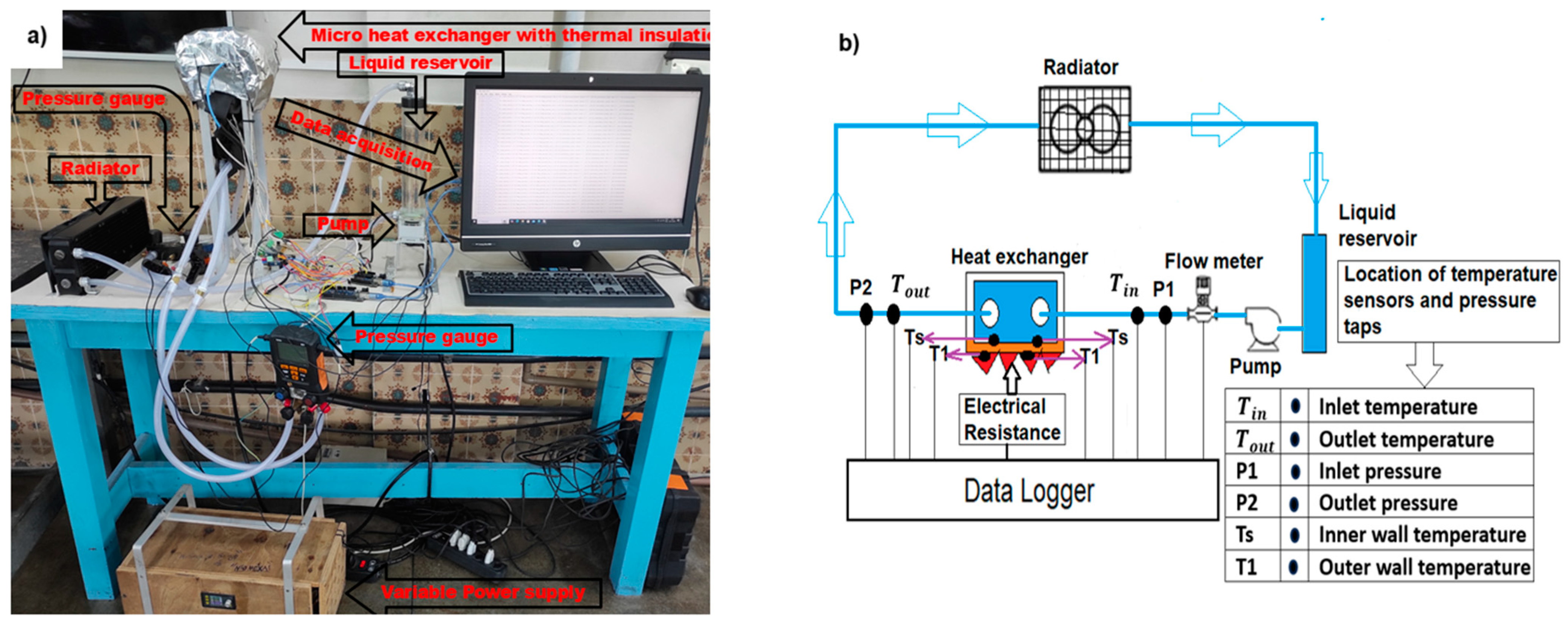
An experimental prototype was developed to assess the performance of a mini heat exchanger designed for cooling electronic components, such as computer processors. Figure 2 shows the configuration of the prototype, comprising (a) the experimental setup (left-one) and (b) the experimental scheme (right one). This setup simulates the thermal load that is typical of electronic components using an electrical resistance. The flow rate can be adjusted using a pump with variable power settings. A variable power supply allows for adjusting and monitoring the power of the electrical resistance, which simulates an electronic component. The mini heat exchanger, electrical resistance, and temperature sensors are thermally isolated. Data on physical quantities are collected via serial or Bluetooth communication using specialized hardware and software for data acquisition [30,31,32,33]. The temperature sensors and pressure taps shown in Figure 2 were strategically positioned to calculate the average convective heat transfer coefficient (h) and the overall thermal resistance of the heat exchanger.
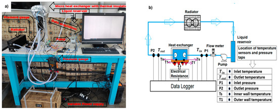
Figure 2.
(a) Experimental apparatus—prototype. (b) Experimental scheme.
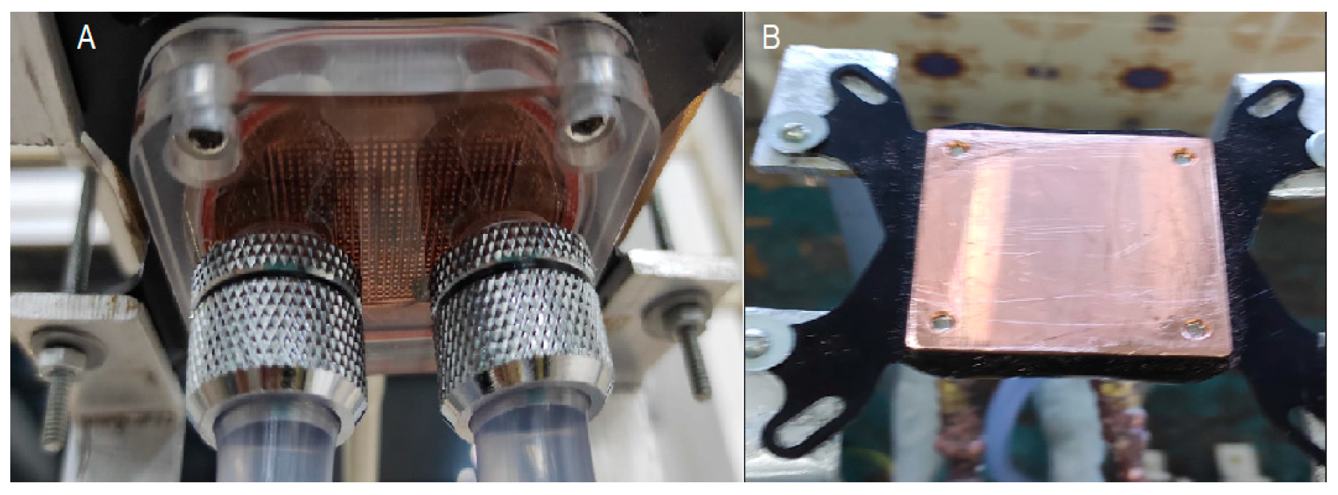
The mini heat exchanger used in the experiment, as shown in Figure 3, is a minichannel model, commonly known as a CPU water cooler block for AMD AM4 processors. It is also compatible with AM3 processors. This heat exchanger is specifically designed to support the AMD Ryzen AM4 processor family, which has a Thermal Design Power (TDP) ranging from 35 W to 65 W, according to the manufacturer’s specifications [23]. Figure 3A,B depict the water cooler block designed to dissipate the heat generated at the CPU by the electrical resistance mounted on top. The components are separated by layers of Kapton tape, which prevents the flow of the electrical current. This mini heat exchanger features G1/4” threads for connecting 3/8” hoses that circulate fluid through its minichannels. This fluid circulation effectively removes heat, cooling both the CPU block and the electronic component, which in this case is an electrical resistance. It is composed of copper and acrylic, with a copper base measuring 0.05 m by 0.05 m.
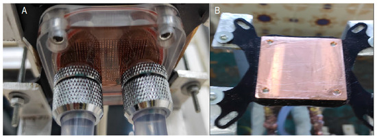
Figure 3.
(A) Minichannel design. (B) Mini heat exchanger for the CPU block.
The electrical resistance installed above the mini heat exchanger was used to simulate the thermal load of an electronic component. This resistance tape measures 5.0 mm by 0.30 mm and has a resistivity of 0.50 ohms. Two thermocouples measured the average surface temperature.
A Barrow-brand reservoir with a diameter of 50 mm and a height of 240 mm was installed in the prototype for deionized water circulation, alongside a 17 W SPB17 Plus pump. Both the reservoir and the pump feature G1/4” threads. The pump is connected to a 12 V DC power source and includes speed control.
The radiator used is a Freezemod TSRP45-BP360 model. It features 12 layers of copper tubes with a 4 mm spacing between the fins. The radiator’s dimensions are 391 mm in length, 121 mm in height, and 45 mm in thickness, and it uses G1/4” threaded connections. This type of radiator is commonly employed in conjunction with CPU block heat exchangers for heat dissipation. Three GS12 fans from the Freezemod brand were installed. Each fan operates at a rotational speed of 2000 ± 10% RPM and has a flow rate of 116.76 m3·h−1, running continuously at 12 V. The dimensions of each fan are 120 × 120 × 25 mm.
2.2. Sensors and Instruments
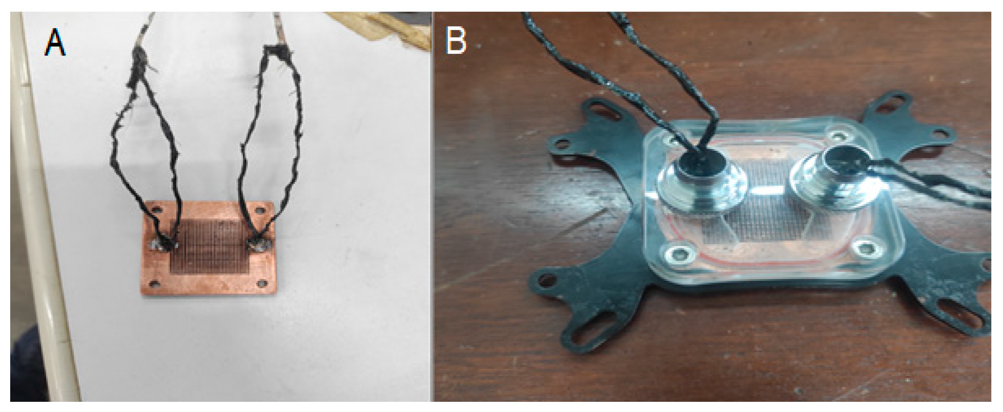
In addition to the two type-K thermocouples placed on the surface heated by electrical resistance, two more type-K thermocouples were installed on the opposite side of the copper surface that contacts the water flowing through the interior of the mini heat exchanger, as illustrated in Figure 4A,B.

Figure 4.
Thermocouples secured with tin solder on the surface. (A) View 1. (B) View 2.
The prototype configuration employed a sandwich-type design, incorporating ceramic plates with thermocouples and electrical resistance sensors pressed against the mini heat exchanger. To connect electrical resistance, a variable power supply, labeled DPS5020, was used. This power supply includes monitoring and data acquisition software that operates via Bluetooth.
Table 1 presents the characteristics and operational parameters of this power supply, allowing for the adjustment of the electrical power supplied to the resistance.

Table 1.
Power supply parameters for DPS 5020.
A DPS5020 power supply was used to monitor and perform the data acquisition. The DHT22/AM2302 humidity sensor was employed to monitor the environmental humidity during the experiment. This sensor has a measurement range of 0 to 100% relative humidity, a power supply requirement of 3 to 5.5 VDC, and an accuracy of ±2% relative humidity (RH).
A hall sensor water flow meter, capable of measuring flow rates between 1 and 30 L, was installed alongside an Arduino board to monitor water flow during the experiment. The meter’s specifications include a maximum working pressure of 1.75 MPa, a maximum water temperature below 110 °C, and an operating voltage range of 5 VDC to 15 VDC.
The Testo 547 digital manifold was utilized to measure the water pressure at both the inlet and outlet of the CPU block-type minichannel heat sink. Additionally, the ambient temperature was recorded using the digital manifold. This manifold features a pressure resolution of 0.1 psi and a temperature resolution of 0.10 °C. The Testo 557 digital manifold showed a temperature accuracy of ±0.50 °C (±1 digit).
2.3. Calibration and Uncertainty Analysis
The uncertainty analysis of the experiments performed was conducted according to the general methodology presented in Appendix A of this article.
Table 2 shows the uncertainties of the quantities used in the experiment. The thermocouple and humidity sensor were calibrated, the flow sensor was calibrated experimentally, and the other uncertainties are manual or propagation uncertainties.
Table 2.
Experimental uncertainties.
2.4. Data Acquisition System
An Arduino Mega 2560 board and an Arduino Uno board were used in conjunction with four K-type thermocouples, a DHT22 humidity sensor, a Hall sensor water flow meter, and two NTC sensors. Data acquisition from the Arduino boards was accomplished using serial communication, integrated with Python 3.10 on an HP Compaq Elite 8300 all-in-one computer. The computer is equipped with an Intel i5-3570 processor running at 3.4 GHz, 16 GB of RAM, and an SSD of 480 GB.
3. Experimental Methodology
The mini heat exchanger and the temperature and pressure measuring sockets were effectively thermally insulated using ceramic fiber, elastomeric rubber, and aluminum foil. This thermal insulation ensured that heat Q flowed in a unidirectional manner from the electrical resistance to the heat exchanger. Figure 5 shows the setup for unidirectional heat transfer [34,35,36].
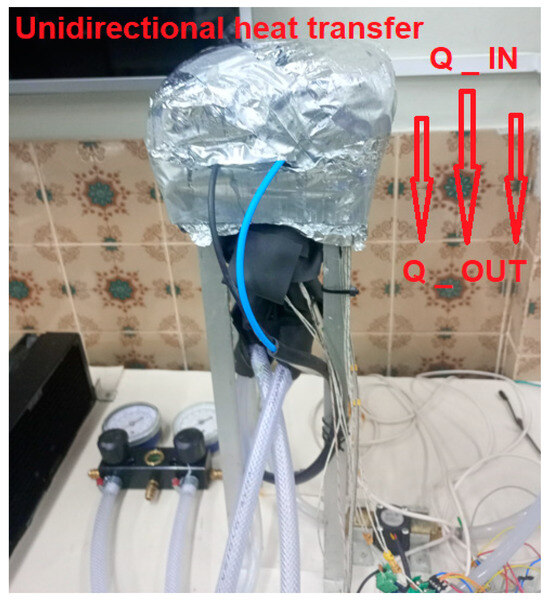
Figure 5.
Thermally insulated mini heat exchanger.
To model heat transfer in the mini heat exchanger, several assumptions were made [34,35,36]:
- Energy balance based on the first law of thermodynamics;
- One-dimensional heat conduction;
- Constant properties, such as thermal conductivity;
- Negligible thermal radiation;
- Negligible heat loss;
- No internal heat generation;
- A uniform convection coefficient;
- Steady-state conditions;
- Fluid incompressible and Newtonian;
- No-slip condition.
These factors simplify the analysis of the heat exchanger’s performance. Fourier’s Law has been applied to assess heat transfer through conduction in the electrical resistance that is in contact with the copper surface of the mini heat exchanger. In one dimension, Su et al. [28] describe the heat transfer scenario using Equation (1) considering the simplifications that have been assumed:
According to the first law of thermodynamics and the simplification of the heat equation [20,22], the heat transferred by electrical resistance (HER) is described by Equation (2), which is conducted to the heat exchanger. This heat then passes through the wall and exits via convection, as explained in Equation (3), inside the mini heat exchanger, which is cooled with water. The fluid in contact with the wall has zero velocity, and heat transfers through conduction before exiting the heat exchanger via convection. The heat transferred by the electrical resistance equaled the electrical power supplied [35], which was monitored every second by the DPS 5020 power supply; however, data were only used from the steady state.
By applying the conservation of energy and rearranging Equation (3), the average convective heat transfer coefficient (h) can be determined using Equation (4) [28,36,37].
For internal flow, the fluid temperature is determined by averaging the inlet and outlet temperatures. Since the difference between these temperatures is small, this average temperature was used to calculate properties such as specific heat, viscosity, density, and thermal conductivity. The water temperature () for these calculations is provided by Equation (5).
The inner wall temperature (Ts) in contact with the water was measured using type-K thermocouples, which were fixed in place with tin solder. Since tin solder has a different thermal conductivity than the copper material of the heat exchanger, a compensation for this effect was necessary. The adjusted temperature difference () that the sensor could measure was calculated according to Equation (6). In this equation, (Ks) represents the thermal conductivity of the tin solder, (Ls) denotes the thickness of the tin solder, (A) is the area, and (Q) is the heat transfer. Although the effect of this discrepancy was minimal, it was nonetheless compensated for in our measurements.
The GTR was determined by subtracting the fluid temperature from the highest temperature of the mini heat exchanger, which is the outer wall temperature (T1) and then dividing the result by the heat (Q), which is equal to (HER) [10,36] as shown in Equation (7).
The thermal circuit is used to calculate GTR, which is determined using Equation (8). This equation accounts for the resulting global thermal resistance from both the solid copper wall of the heat exchanger and the resistance of the fluid. As expected, the result obtained was consistent with the outcome from Equation (7).
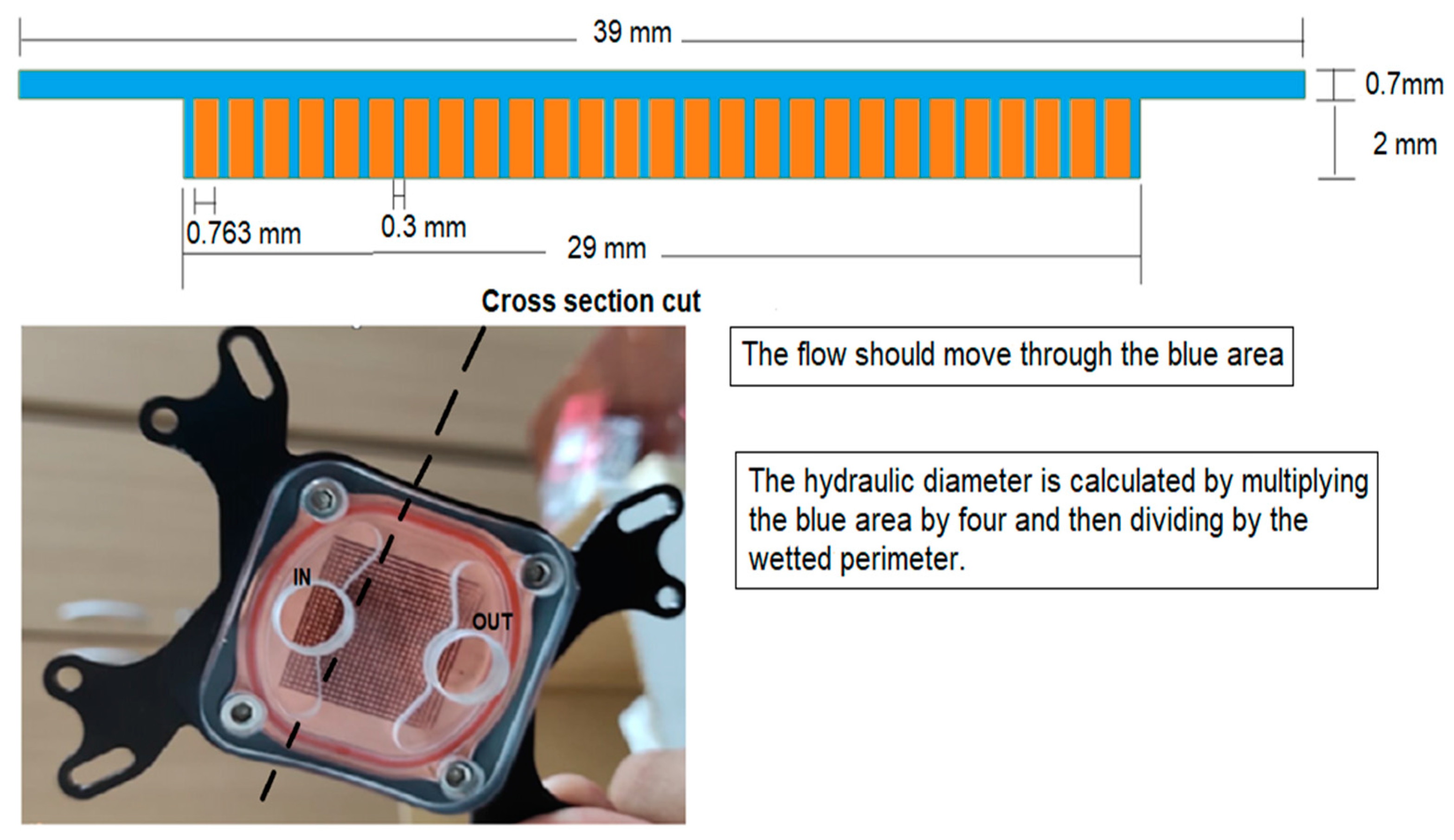
The hydraulic diameter () is determined by first calculating the cross-sectional area (), multiplying that area by 4, and dividing the result by the wetted perimeter (P). This process is expressed in Equation (9) and illustrated in Figure 6. The hydraulic diameter is the characteristic length of the geometry [38], which is essential for calculating the Reynolds number. This calculation helps to identify whether the fluid flow regime is laminar with a Reynolds number below 2100, as is the case in this study, transient with a Reynolds number above 2100 and below 4000, or turbulent with a Reynolds number above 4000. The hydraulic diameter was determinate based on Equation 9, as found in the literature [28,39].
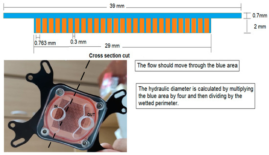
Figure 6.
Hydraulic diameter procedure.
To facilitate the study of minichannel heat exchangers and assess the scale effect, Kandlikar and Grande [38] developed criteria for categorizing minichannels based on their hydraulic diameter (). The classifications are as follows:
- Transitional channel: 0.1 µm < Dh < 10 µm;
- Microchannel: 10 µm < Dh < 200 µm;
- Minichannel: 200 µm < Dh < 3 mm;
- Conventional channel: Dh > 3 mm.
The heat exchanger examined in this study falls into the minichannel category, with a hydraulic diameter of 832 µm.
In Figure 6, a cross-section of the heat exchanger is illustrated. The blue area represents the cross-sectional area through which the fluid flows, denoted as , and is used to calculate the hydraulic diameter. The solid copper section of the heat exchanger is depicted in orange. The fluid in blue is enclosed by the remainder of the heat exchanger, which is constructed from acrylic. The portion of the cross-sectional area where the fluid comes into contact is referred to as the wetted perimeter (P).
The Reynolds number is calculated by multiplying the density of the fluid (ρ), velocity (V), and characteristic length of the geometry (), in this case, the hydraulic diameter. This product is then divided by dynamic viscosity (µ), as shown in Equation (10).
In the experiment, the velocity used to calculate the Reynolds number was derived from the volumetric flow rate and the cross-sectional area. The dynamic viscosity applied in the calculations was determined based on the average temperature and pressure of the fluid, whereas the density was dependent on the average temperature of the fluid. During the experiment, measurements were taken of the ambient temperature, volumetric flow rate, inlet and outlet pressure of the heat exchanger, and relative humidity. All data regarding physical quantities were collected exclusively under steady-state conditions; measurements obtained during transient states were not utilized in any calculations for this study.
Basic Principles in FFD Building
In chemometric applications, it is essential to set the levels of these factors correctly to ensure that the response variable is maximized. This process involves finding the ideal levels for each factor. Thus, before beginning the optimization process, it is necessary to identify which factors and respective interactions significantly impact the response variable. It is also beneficial to determine which factors have minimal or no effect to avoid wasting time and resources on unnecessary experiments. All calculations and graphical analyses were performed with the Statistica® software package, version 6 [40]. The statistical significance of the results was tested at the p < 0.05 level.
In this study, the choice of factors was based on their expected impact on the heat dissipation efficiency, evaluated by the GTR (°C·W−1) and the convective heat transfer coefficient h (W·m−2·°C−1). Therefore, power supply, temperature, and flow rate (labeled as A, B, and C, respectively, in Table 3) were identified as key variables that could influence cooling efficiency (23 FFD). For two-level designs, it is customary to identify the higher and lower levels with (+) and (−) signs, respectively. These levels were determined based on practical operating ranges and prior knowledge of the system. This binary coding simplifies the chemometric treatment of data, allowing for the straightforward calculation of main effects and their interactions.
Table 3.
Factors and levels of the 23 FFD.
In this setup, we have three factors, each with two levels, resulting in 23 = 8 combinations. The GTR and values observed from these runs, which were conducted in a random order and in duplicate (for a total of 16 experiments), are presented in Table 4, in which the design matrix and results of the full 23 designs are displayed. The number in parenthesis following each response value indicates the order in which the run was conducted.
Table 4.
Design matrix and results of the full 23.
In experimental design, particularly in factorial experiments, a contrast matrix is a powerful tool for analyzing the main effects and interactions between factors. Constructing a contrast matrix involves defining the factors and levels, creating a design matrix of all possible combinations, adding columns for main effects and interactions, and then interpreting these columns to understand the significance of each factor and interaction. To form a contrast matrix, new columns for the main effects and interactions (Table 3) are required, in which the effect or interaction is represented by a new column.
The main effects of factors A, B, and C are straightforward, but it is also important to consider the two-factor interactions (AB, AC, BC) and the three-factor interaction (ABC). The signs in these interaction columns are determined by multiplying the signs of the relevant factors. For instance, the column for interaction AB is generated by multiplying the signs from the columns for A and B.
Similarly, the column for the three-factor interaction ABC is the product of the signs from the columns for A, B, and C, as illustrated in Table 5. This table presents the contrast matrix for the 23 factorial design. The last column contains the average values of GTR and h obtained from the experimental runs, as shown in Table 4.
Table 5.
Contrast matrix for the 23 factorial design.
Conducting this factorial design and calculating the main effects and interactions allows for a comprehensive assessment of the influence of each factor and their combinations on the responses. The duplication of experiments enhances the robustness of the results, providing a reliable statistical framework for understanding the significant parameters affecting the industrial cooling process.
4. Analysis and Discussion of Results
In this section, a thorough analysis and discussion is conducted based on observations, comparisons of experimental results, and relevant theories on the subject studied.
4.1. Full 23 Factorial Analysis
The calculation of the main effects and interactions involves comparing the average responses at the high and low levels of each factor. The main effect of a factor is the difference between the average response at the level (+) and the average response at the level (−) of that factor.
Thus, to quantify the main effect of the power supply (factor A) on the GTR, for instance, Equation 10 should be used:
In Table 5, represents the response for the ith entry, resulting in . In a similar way, it is possible to calculate the main effects of factors B (temperature) and C (flow rate) for both responses (GTR and ). The interaction effects between the factors can also be determined by examining their combined effects.
To calculate the interaction effect between factors A and B, we analyzed the difference between the average response values (using h as an example) at the high level (entries 1, 4, 5, and 8 in Table 5) and at the low level (entries 2, 3, 6, and 7). By applying this reasoning, all the effects of two-factor and three-factor interactions were determined. The values are presented in Table 6. The values in red indicate statistical significance at the 95% confidence level.
Table 6.
Estimates of the main and interaction effects.
In statistical analysis, it is necessary to decide which effects are significant and different from zero, and therefore worthy of interpretation. First, the effect whose absolute value is greater than t8 × seffect was considered statistically significant. The parameter t8, used to determine the significance threshold for the effects, originates from the t-distribution, which is commonly employed in statistical hypothesis testing. The value t8 = 2.306 corresponds to the critical t-value for a two-tailed test with eight degrees of freedom (from the design matrix, df = N − k, where N is the number of experimental runs and k is the number of model parameters), at a 95% confidence level (α = 0.05). This critical value is then multiplied by the standard error of the effect (seffects) to establish the minimum magnitude that an effect must be considered as significantly different from zero. This ensures that only effects with a sufficiently large impact, beyond random experimental variability, are interpreted as statistically relevant.
In this context, for the GTR, an effect will be considered significant if its value exceeds t8 × seffect = 2.306 × 9.246 = 21.321. Conversely, when considering h as the response variable, the effect becomes statistically relevant if its value is greater than t8 × seffect = 2.306 × 9.842 = 22.697. Applying this interpretation to the effects shown in Table 6, the significant factors were the power supply (Table 6, entry 1) for GTR, and temperature followed by power supply, in order of importance (Table 6, entries 1 and 2) for h. Additionally, the Pareto chart (Figure 7) can be used to illustrate which main effect is most significant. The effects whose rectangles are to the right of the dividing line should be considered in the statistical model, as they represent values greater than p = 5% (95% confidence interval). In this context, once again the only main factor with statistical relevance for thermal resistance is the power supply (Figure 7a), whereas for h, the significant factors are the power supply and temperature (Figure 7b). The values next to the rectangles represent the values of the t-test statistics obtained in the main effects window. In statistical terms, the other main effects (flow rate and temperature for GTR, and flow rate for h), as well as any of the two- or three-factor interactions, can be regarded as inert factors in these experiments and should therefore be disregarded in the experimental analysis.
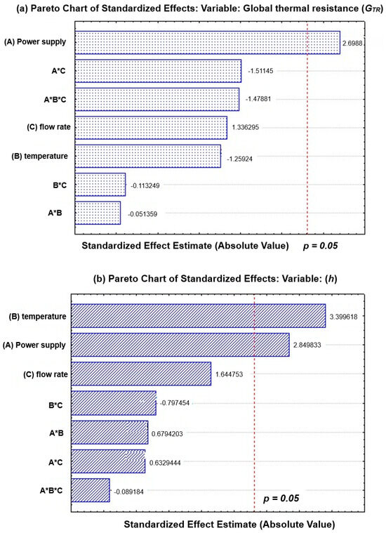
Figure 7.
Pareto chart as a function of the values of the t-test statistics: (a) GTR and (b) .
4.2. Interpretation of the Effects
This section assesses the impact of three variables—the volumetric flow, ambient temperature, and power source (dissipated power) of the electronic component, specifically the electrical resistance—on two response variables, GTR and the heat transfer coefficient (h). Table 7 presents the results of the statistical evaluation concerning the variation in the levels of these three variables and their consequences on the response variables.
Table 7.
Effects of the statistical evaluation.
4.2.1. Global Thermal Resistance (GTR)
The effect of a factor is defined as the change in the response (GTR or h) when it is moved from a lower level (−) to a higher level (+). Considering that the power supply (factor A) is the only statistically significant factor for the GTR response (Table 6—entry 1, and Figure 7a), it is observed that the change from the level (−) to the level (+) of factor A (30 W to 65 W) increases the thermal resistance, on average, by 24.954 × 10⁻³ °C·W−1.
The temperature effect is negative, indicating that increasing the temperature from a low of 22 °C to a high of 29 °C reduces thermal resistance, on average, by 11.643 ± 0.9 °C·W−1. While this result aligns with the goal of decreasing thermal resistance, the t-test and Figure 7a show that the effect is not statistically significant at a 95% confidence level. This suggests that, although the temperature change may have a beneficial impact, it is not consistent enough to be considered reliable within the temperature range tested in the experiment.
The flow rate is not statistically significant, and its effect is positive (12.356 ± 9.3 × 10⁻³ °C·W−1), indicating that increasing the flow rate from its low (2.5 L/min) to high level (5 L/min) increases the thermal resistance. Finally, none of the interactions (AB, AC, BC, or ABC) are statistically significant (Figure 7a and Table 4). This suggests that combinations of factors do not have a meaningful impact on thermal resistance within the levels tested.
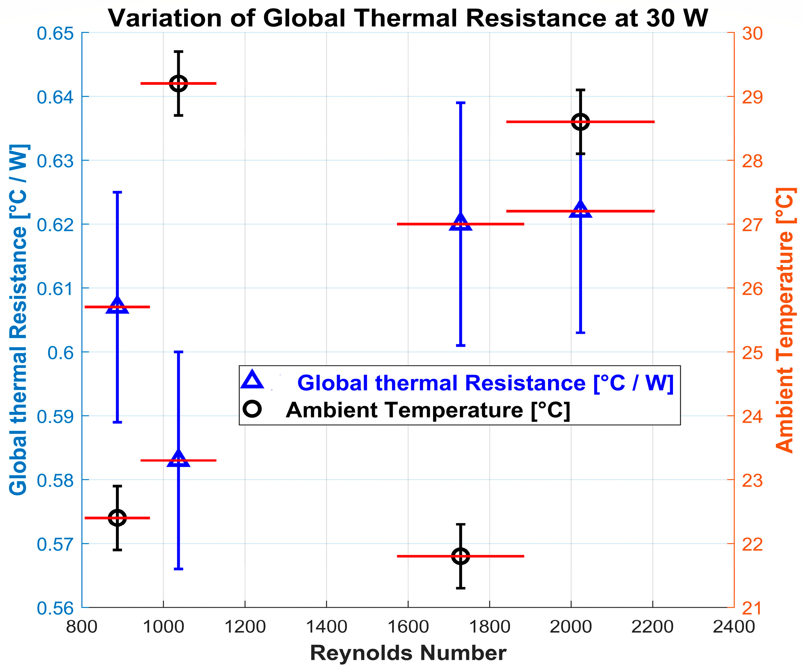
Figure 8 and Figure 9 show the average increase in global thermal resistance at the dissipated power levels 30 W and 65 W as a function of the Reynolds number and the ambient temperature. Two of the three variables that were varied to assess the response of global thermal resistance were ambient temperature and volumetric flow rate.
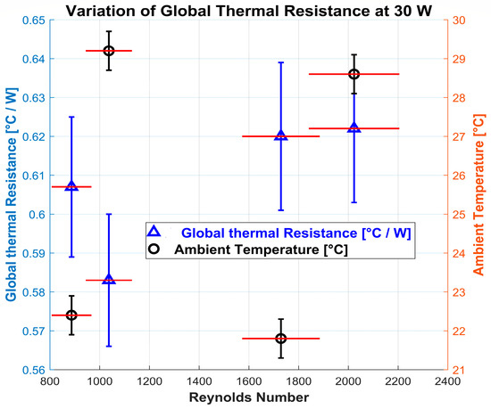
Figure 8.
Global thermal resistance and ambient temperature at the power level of 30 W.
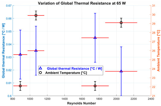
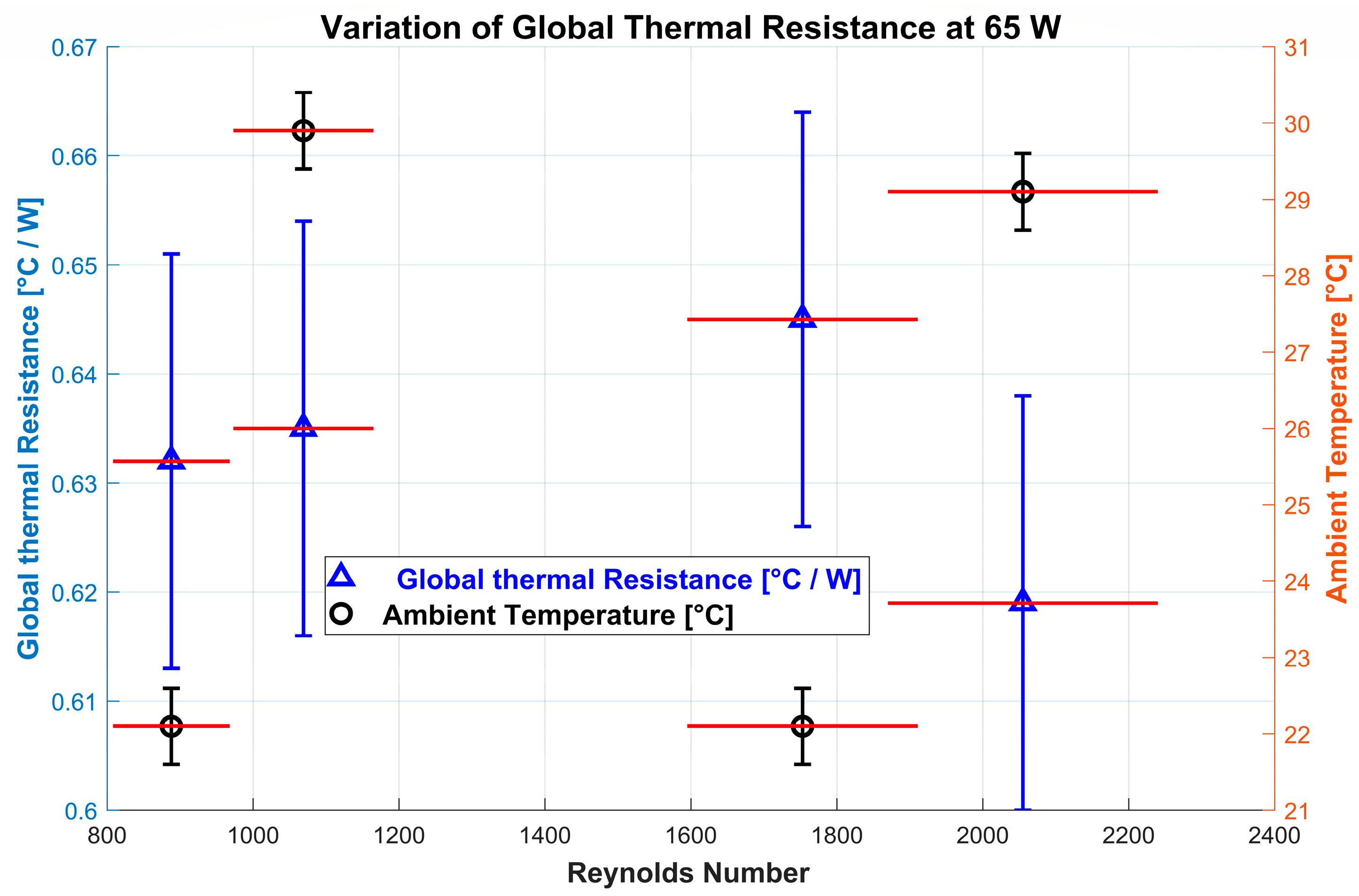
Figure 9.
Global thermal resistance and ambient temperature at the power level of 65 W.
The Reynolds number increases with higher volumetric flow rates. It is also affected by ambient temperature due to the changes in water temperature that ambient temperature induces, which alters properties influencing the Reynolds number, such as viscosity and density.
The analysis conducted within the range of variables in this experiment shows that only power significantly impacts the variations in thermal resistance. From the analysis and Pareto chart (see Figure 7), changes in volumetric flow rate or temperature do not have a significant effect on thermal resistance. Hence, adjusting the volumetric flow rate and ambient temperature within the specified range will not improve performance. Utilizing a lower-power pump may be a feasible option to reduce costs or energy spending on the equipment/to optimize the use of electrical energy in the system.
As shown in Figure 9, higher Reynolds numbers correspond to improved thermal resistance. Nevertheless, the design of minichannels incorporating interrupted fin walls may result in the onset of an early transient regime. This characteristic, combined with turbulence and increased power, results in a higher heat transfer coefficient (h) and a decrease in thermal resistance.
4.2.2. Heat Transfer Coefficient (h)
The response variable heat transfer coefficient (h) indicates better performance at higher values. The analysis of the factorial effects reveals that temperature (B) has the largest positive effect (Table 6 and Figure 7b), indicating that increasing the temperature from its low (22 °C) to high level (29 °C) significantly increases h by 33.462 ± 9.8 W·m−2·°C−1, on average. This effect is statistically significant (Figure 7b), making temperature the most influential factor for improving h.
The power supply is statistically significant (Table 6 and Figure 7b), confirming its importance for enhancing performance. This factor also shows a positive effect, suggesting that using 65 W improves h by 28.050 ± 9.8 W·m−2·°C−1, on average. Otherwise, the flow rate has a smaller positive effect in the h, as shown (16.189 ± 9.8 W·m−2·°C−1) and is also not statistically significant. None of the interaction terms are statistically significant, indicating that the combined effects of factors do not meaningfully affect h in this experimental setup.
Therefore, to maximize h, all factors should be adjusted to their highest levels, including a high-power supply, high temperature, and high flow rate. This combination leverages the positive main effects of all factors, particularly the significant contributions of temperature and power supply.
Based on the preference for minimizing thermal resistance as the operational and commercial criterion for evaluating heat dissipation performance, the recommended levels of the factors would prioritize configurations that achieve the lowest GTR. From the earlier analysis, the optimal levels for minimizing thermal resistance were Power Supply (Low, 30 W), Temperature (High, 29 °C), and Flow Rate (Low, 2.50 L·min−1). This combination reduces the thermal resistance, ensuring that the heat sink is more effective at transferring heat away from the electronic component, which is critical for practical applications such as heat sink design and selection.
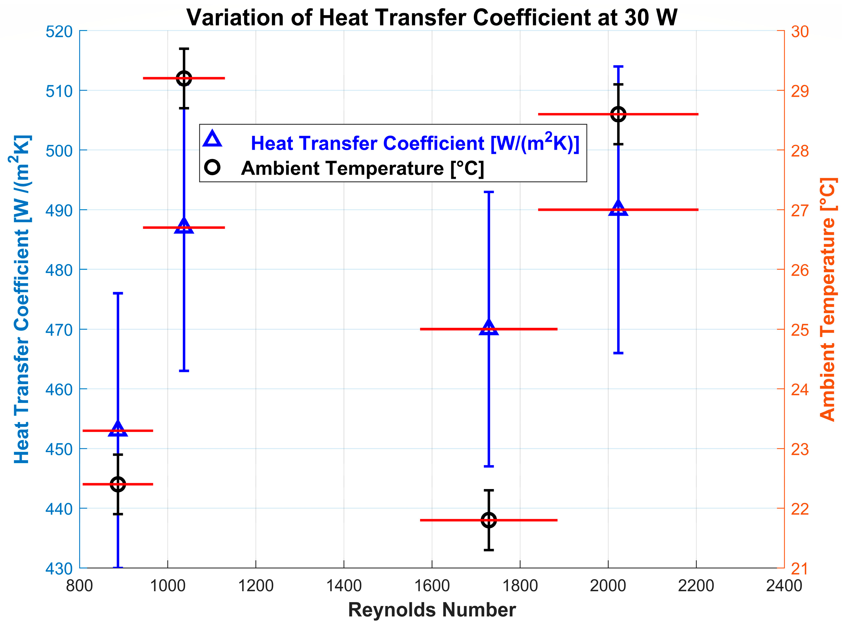
Figure 10 and Figure 11 display the average increase in the heat transfer coefficient (h) as the dissipated power levels of 30 W and 65 W and the ambient temperature (range of 22 °C to 29 °C) with the Reynolds number. It is important to note that the volumetric flow rate does not significantly affect the changes in within this range. The Reynolds number is included because it rises with an increase in the volumetric flow rate, and the ambient temperature also has an effect due to its relationship with variations in water temperature, as well as changes in density and viscosity, which are used in the Reynolds number calculation.
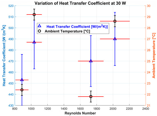
Figure 10.
Heat transfer coefficient and ambient temperature at the power level of 35 W.
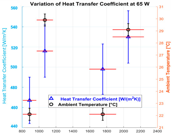
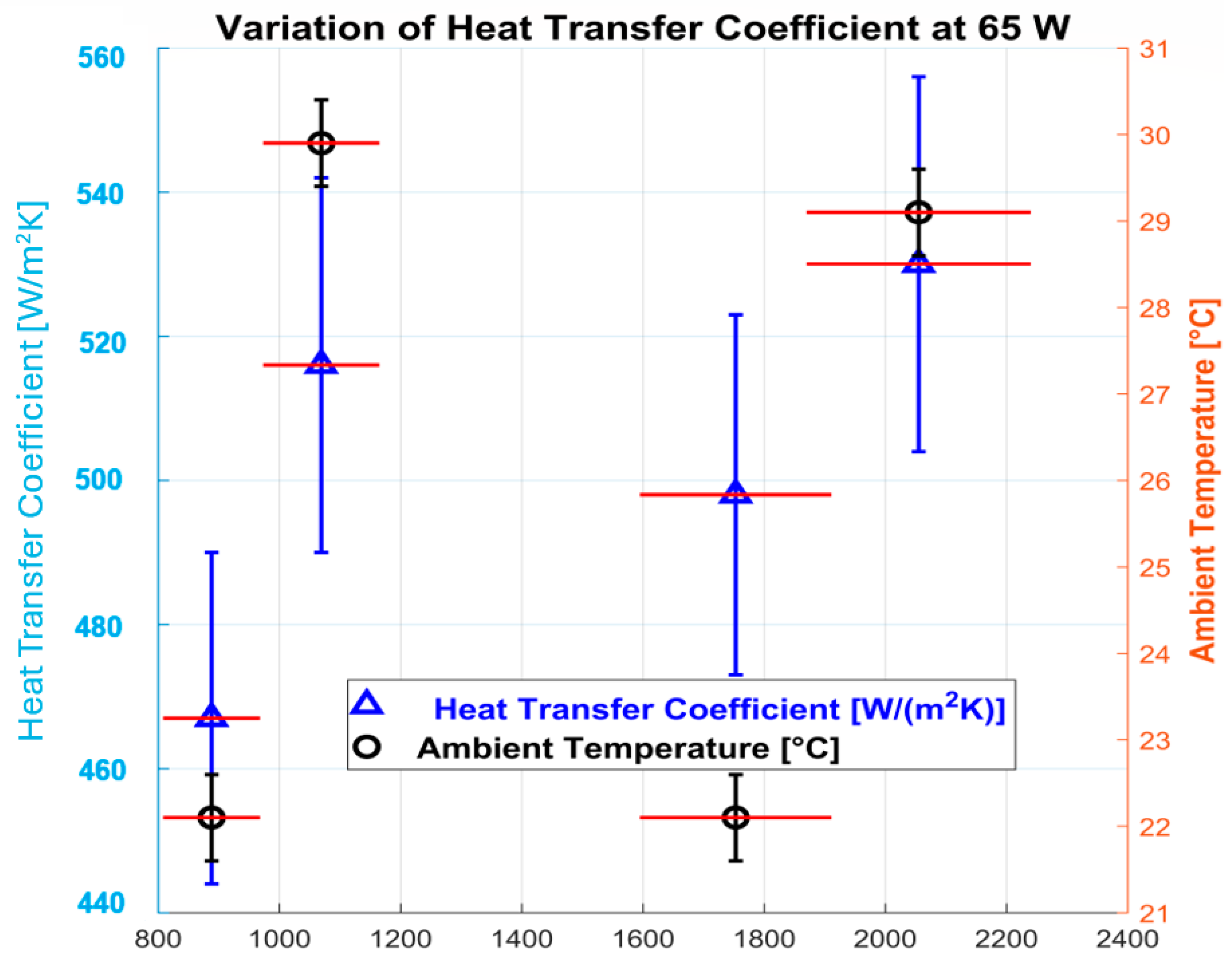
Figure 11.
Heat transfer coefficient and ambient temperature at the power level of 65 W.
Figure 11 supports the explanation given in Figure 9 regarding the improvement in global thermal resistance at a heat dissipation level of 65 W and at high Reynolds numbers. This enhancement in heat transfer coefficient, accompanied by a decrease in thermal resistance, may be attributed to an earlier transition from laminar to turbulent flow regimes. The results showed that the heat transfer coefficient increased with higher dissipated power, consistent with the findings of Manikandan [41], who investigated the influence of nanofluids on heat transfer in a natural convection system.
4.2.3. Comparison of Optimal Conditions
According to the experimental analysis, the optimal temperature (B: high) aligns for both responses (GTR and ), indicating that increasing temperature consistently improves system performance. However, the power supply (A) shows conflicting behaviors. A low level minimizes GTR, but a high level maximizes h. This reflects a trade-off between these variables. The flow rate (C) has a limited influence on both responses, but for h, the high level is preferred.
For a complementary analysis, where the focus is on maximizing the convective heat transfer coefficient (h), the optimal configuration involves all factors at their high levels: Power Supply (High, 65 W), Temperature (High, 29 °C), and Flow Rate (High, 5 L·min−1). This setup provides the highest h, indicating enhanced heat exchange efficiency. However, this is less critical for operational and commercial applications compared to thermal resistance. In addition, the volumetric flow rate, despite not presenting statistical significance, had a positive contribution to the heat transfer coefficient, evidencing that the increase in turbulence can be explored for additional thermal gains, as highlighted in the literature [28,38].
4.2.4. Mini Heat Exchanger Performance
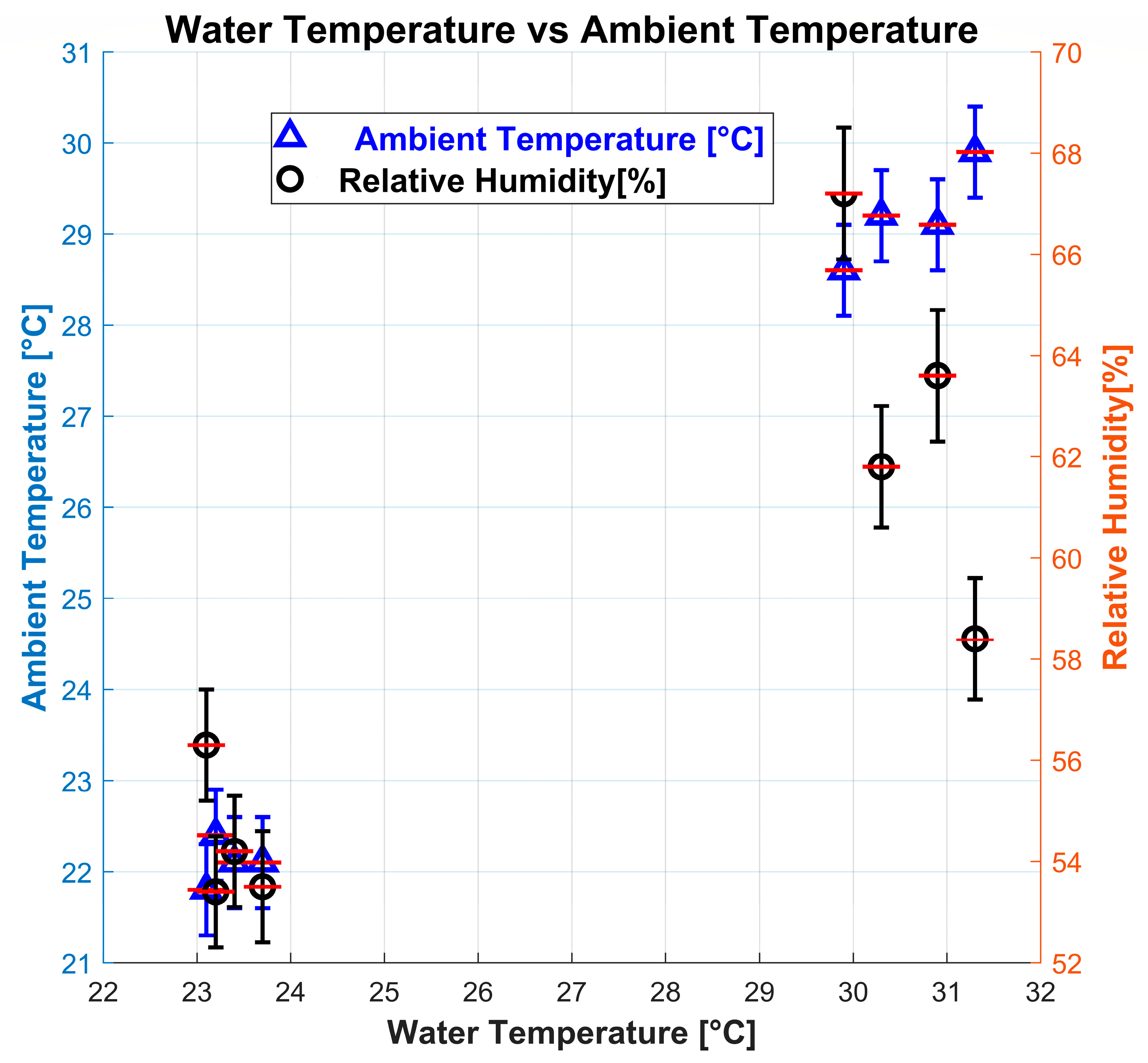
The GTR enables the measurement of the heat dissipated from an electronic component to maintain the optimal operating temperature. As the electrical power of this component increases, both the heat transfer coefficient and the thermal resistance also rise. In the analysis, only variations in power had a significant impact on overall thermal resistance. However, both power and ambient temperature were statistically significant for the heat transfer coefficient (h). This is attributed to the relationship between ambient temperature (relative humidity) and the water temperature, which alters the thermophysical properties and leads to changes in heat transfer. Relative humidity influences air density and viscosity, impacting the convective heat transfer coefficient of air. Higher humidity enhances thermal capacity, while lower humidity reduces it, underscoring the role of air moisture in heat transfer. This is particularly pertinent since water cooling in the radiator relies on ambient air for heat dissipation. Furthermore, Figure 12 confirms that both temperature and relative humidity were measured, ensuring a comprehensive evaluation of all factors influencing heat transfer and reinforcing the reliability of the data collection.
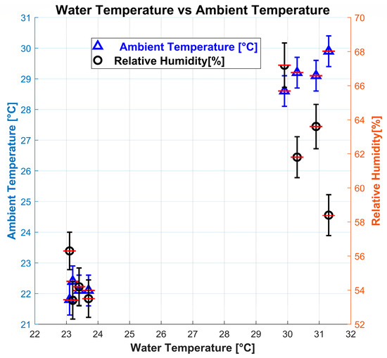
Figure 12.
Effect of ambient temperature and relative humidity on (T∞).
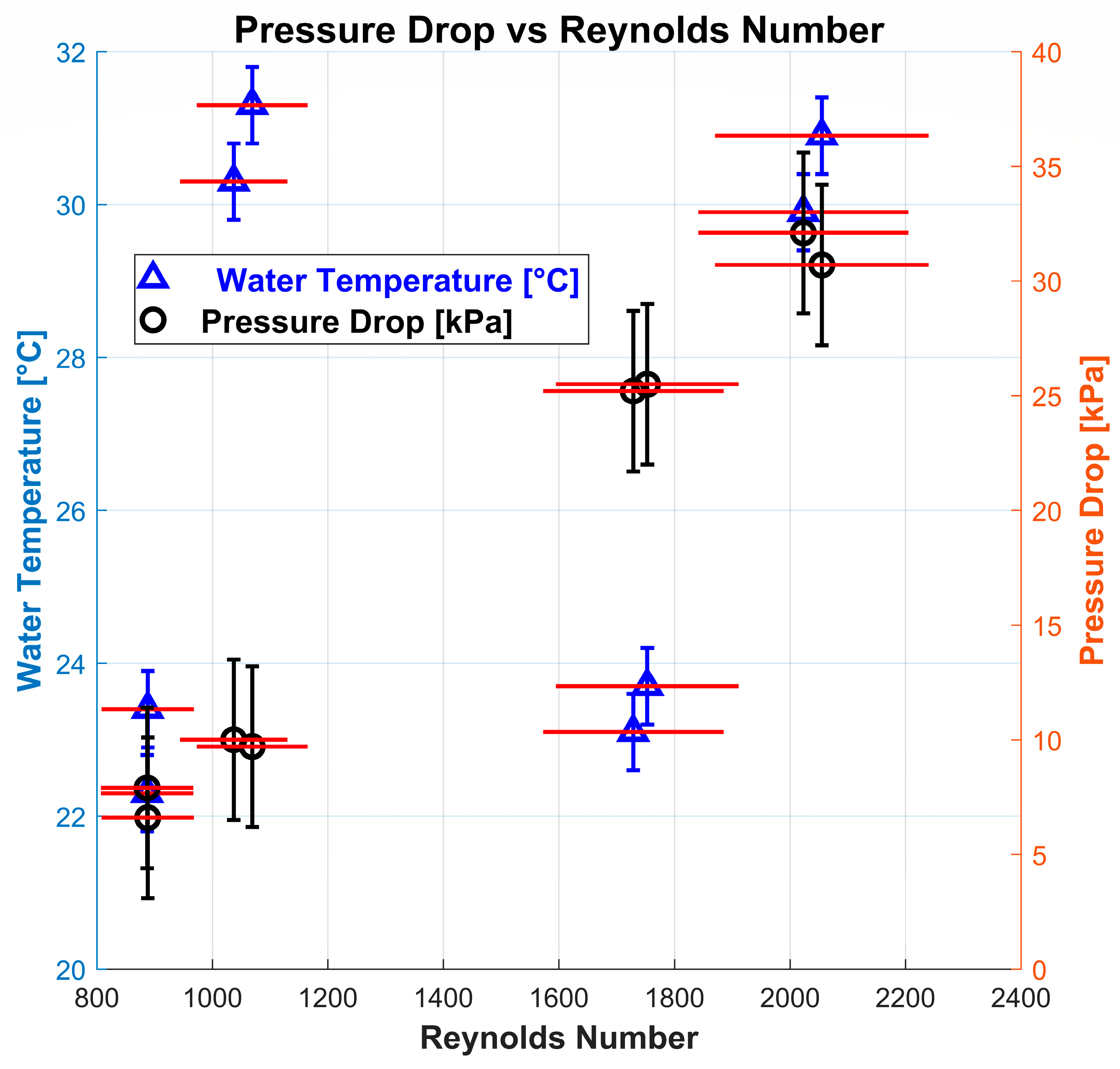
Figure 13 shows the pressure drop in the heat exchanger. Although the pressure drop increases as the volumetric flow rate rises, resulting in higher velocities and a higher Reynolds number, the pressure drop in the heat exchanger will continue to increase progressively. This occurs since the pressure drop is directly proportional to the Reynolds number. As the volumetric flow rate increased, the fluid velocity also increased, which led to a higher Reynolds number and, consequently, more significant pressure drops due to increased viscous friction.
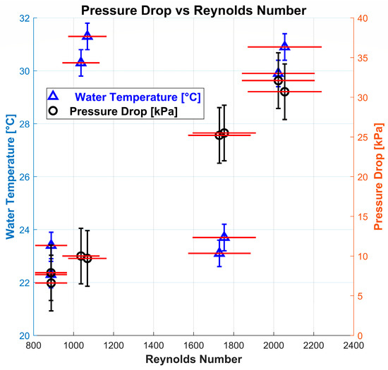
Figure 13.
Water temperature and pressure drops in the mini heat exchanger.
It is essential to enhance the heat transfer coefficient (h) to improve heat dissipation and reduce the overall thermal resistance (GTR), as indicated by Equations (2)–(8). In the experiment, the heat transfer coefficient (h) reveals a limitation in thermal dissipation when thermal power reaches its maximum level. This occurs because the overall thermal resistance increases, hindering the necessary heat transfer to achieve the desired operating temperature of electronic components, such as the Central Processing Unit (CPU). However, within the established conditions and ranges, the overall thermal resistance of this heat exchanger could facilitate the heat dissipation of a processor with a Thermal Design Power (TDP) of 65 W, as analyzed in this study. Consequently, the temperature of the CPU case would be close to the temperature of the outer wall (T1) of the mini heat exchanger, as illustrated in Figure 14. Statistical analysis revealed that the optimal operating conditions for the electronic component within the study range were achieved at a low power level (30 W), a high ambient temperature (29 °C), and a low volumetric flow rate (2.50 L·min−1). However, the highest power condition (65 W) is also viable, as shown in Figure 11, where the maximum outer wall temperature remained below 73 °C, which is an acceptable threshold according to the thermal profiles of most processors [3,31,33,42]. The highest temperature was recorded under warmer conditions, with an ambient temperature of 22 °C resulting in an average outer wall temperature of 66 °C when using a power of 65 W.
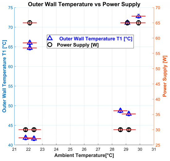
Figure 14.
Behavior of the outer wall temperature, power supply, and the ambient temperature.
4.3. Critical Considerations on the Dissipation Phenomenon in the Prototype
The prototype developed yielded significant results concerning heat dissipation in mini heat exchangers used in electronic components, enabling a critical analysis of the factors most influencing thermal performance. In terms of practical application, this study investigates various residential processors with a Thermal Design Power (TDP) of 65 W, a value attained only under maximum load conditions. During light tasks, power consumption typically decreases to approximately 30 W. Inadequate cooling of a processor can result in performance degradation or even failure, as documented in the literature [1,43].
Among the operational parameters evaluated, electrical power stood out as the most relevant factor in estimating GTR. Increasing power from 30 W to 65 W resulted in an approximate increase of 25 × 10⁻3 °C·W⁻1 in GTR (Table 6), a behavior that can be attributed to the higher thermal flux density under high power conditions. This impact had already been identified in previous studies, which highlight the direct relationship between high power and increased GTR [10,12]. To mitigate this effect, optimized configurations, such as the use of modified surfaces or nanostructures, represent promising opportunities for future improvements [12].
This study investigates methods to enhance cooling and identifies optimal thermal performance conditions within the analyzed range. Two studies on the thermal performance of heat exchangers, employing factorial analysis and the design of experiments, showed that a higher Reynolds number enhances heat transfer, which is consistent with previous research [10,44]. The experiment confirmed that the Reynolds number remained within the laminar regime, where heat transfer is mainly limited by weak convection and dominated by conduction within fluid layers that exhibit minimal mixing. However, at higher Reynolds numbers—under a heat transfer rate of 65 W and elevated ambient temperatures—a significant reduction in thermal resistance was observed. This suggests a transition from a laminar to a transient flow, influenced by factors such as decreased fluid viscosity due to increased temperature and the heat sink’s channel geometry, which features interrupted fins that generate localized vortices. In the transient regime, enhanced fluid mixing leads to improved heat exchange via convection compared to the laminar regime.
On the other hand, although ambient temperature was not statistically significant for the GTR, it proved to be a key factor in enhancing the heat transfer coefficient (h). Under the operating conditions and intervals of the experiment, one viable strategy for improving heat dissipation is to increase the heat transfer coefficient (h) [7,45]. This approach would help mitigate the rise in power of the electronic component from increasing GTR. The temperature increase from 22 °C to 29 °C resulted in an average improvement of 33.46 W·m⁻2·°C⁻1 (Table 6), which is consistent with studies indicating that higher temperatures reduce fluid viscosity, thereby optimizing the thermophysical properties of the system [10,23]. Another key observation is the impact of ambient temperature. The studied range suggests that higher ambient temperatures, which in turn raise water temperature, can enhance the heat transfer coefficient. This is supported by Beck et al. [46] who demonstrated through a numerical study that increasing a fluid’s temperature reduces its viscosity while improving thermal conductivity, ultimately enhancing the heat transfer coefficient (h).
As contextualized in the state of the art [14,15], a fractional factorial design (FFD) outperforms the classical OFAT method by allowing the simultaneous analysis of factors and their interactions, which the OFAT method does not achieve. An FFD offers greater statistical efficiency, a comprehensive exploration of the experimental space, and more accurate estimates, contributing to more robust predictive models. The analysis of the interactions between the operational factors did not reveal statistical significance, suggesting that the individual optimization of each parameter is sufficient to improve thermal performance. In this sense, the literature highlights the importance of prioritizing energy efficiency and minimizing thermal losses to achieve better results [12].
The temperature difference between the electronic component and its surrounding environment is directly proportional to thermal resistance and the heat transfer rate. Reducing thermal resistance throughout the entire heat transfer circuit is essential for optimizing thermal performance. One approach to enhancing this experiment involves minimizing contact resistance to evaluate its impact on thermal efficiency [43].
Unlike previous experimental approaches which relied on parametric studies [7,15], this proposal identified statistically significant variables affecting the efficiency of mini heat exchangers. It demonstrated that the power supply is the dominant factor influencing the GTR, while the ambient temperature significantly impacts h. These findings are consistent with previous research highlighting the importance of energy-efficient heat dissipation in miniaturized electronic devices [8,14]. Additionally, this study provided experimental validation of theoretical predictions, enhancing previous work that primarily relied on numerical simulations [25,26,27].
Finally, the limitations observed in the prototype, particularly under high power conditions (65 W), highlight the need to explore alternatives such as optimized minichannel geometries, higher thermal conductivity materials, and TPMS-based methods (Topologically Optimized Porous Media Structures), as suggested by [7,36]. These approaches can expand the potential for applications in high-thermal-density systems, especially in miniaturized electronic devices. Potential alternatives include modifying the fluid [10,30], increasing the heat exchange area [9], or altering the geometry [9,23,30,35] to improve (h) and reduce the temperature difference between the fluid and the heat exchanger to enhance the heat transfer coefficient.
4.4. Advances in Heat Transfer Through Micro/Minichannels for Cooling Integrated Circuits: Emerging Phenomena and Experimental Challenges
Due to the increasing miniaturization in the integrated circuit industry, microchannels and minichannels are essential solutions for heat dissipation in high-density electronics. The aspect ratio (height/width) influences the flow and heat transfer. Studies indicate that low values reduce thermal efficiency in rectangular and elliptical geometries [47,48], while high values can compromise the performance of heat exchangers, requiring optimization [47]. In the mini exchanger of this study, heat transfer occurs in a combined manner, with interaction between conduction, convection, and adjacent channels.
Recent research proposes strategies to improve heat transfer, such as asymmetric barriers, fins, mixed-wetting surfaces, and nanofluids. When applied to optimized heat sinks, hybrid nanofluids increase efficiency by up to 72% [49]. Three-dimensional heat exchangers with vortex generators perform superiorly to conventional microchannels [50]. The findings of this study corroborate such advances, with global thermal resistance (GTR) reduced to 606.6 × 10⁻3 °C·W⁻1.
Minichannels, operating between laminar and turbulent regimes, exhibit distinct thermal behaviors. Structured geometries and textured surfaces improve dissipation by influencing secondary flow [25]. The results of this study confirm that flow rates and power impact heat transfer in minichannels.
The transition to the microscale introduces new thermal phenomena, such as early turbulence, confinement, and changes in boiling. Spatial confinement influences bubble nucleation and growth [51]. Likewise, this study observed that high Reynolds numbers reduce thermal resistance at high powers (65 W), corroborating the literature [6,7,25]; factors such as fluid ingress and non-uniform distribution impact thermal performance in minichannels. Surface roughness and wettability gradients affect heat exchange, as demonstrated in this study [46]. Experimental validation of heat transfer in micro- and minichannels still faces challenges due to geometric accuracy and limitations at the microscale [52]. Due to nanoscale effects and flow instabilities, traditional models have difficulty predicting thermal resistance and convective coefficients [53]. In this study, the application of a full factorial design (FFD) allowed for the statistical evaluation of the main parameters that affect GTR and h. Differently from the one-factor-at-a-time (OFAT) method [14,15], the FFD revealed that power was the most relevant factor for GTR, while ambient temperature influenced h [16]. Optimization strategies such as customized flow rates and power input control demonstrated improvements that were comparable to more complex structural solutions [25]. These findings reinforce the importance of robust experimental methodologies and highlight the need to explore nanostructured surfaces and additive manufacturing for thermal optimization.
5. Conclusions
This study presented a systematic approach to analyzing thermal dissipation in mini heat exchangers, highlighting the impact of three main operational variables: power source, ambient temperature, and volumetric flow rate. The use of the full factorial design (FFD) method allowed for the comprehensive evaluation of the individual effects and interactions of these variables on the performance parameters: global thermal resistance (GTR) and the heat transfer coefficient (h). The results showed that electrical power was the most significant variable for GTR, while ambient temperature was also a determining factor for the heat transfer coefficient. On the other hand, the volumetric flow rate did not present relevant statistical significance for any of the response variables within the studied range. In addition, the following key findings were observed:
- ✓
- The minimization of global thermal resistance was achieved with the reduced power (30 W), high ambient temperature (29 °C), and low volumetric flow rate (2.50 L/min).
- ✓
- The maximization of the heat transfer coefficient was obtained at high power (65 W), high ambient temperature (29 °C), and a high volumetric flow rate (5 L/min).
- ✓
- The methodology developed, which included the assembly of a prototype and detailed statistical analysis, establishes a reference standard for future studies. However, it is recommended that other temperature, power, and flow ranges be investigated to validate the results in different contexts and potentially optimize refrigeration systems.
- ✓
- These findings highlight the importance of striking a balance between thermal performance and energy efficiency, which is a critical factor for optimizing the functionality of miniaturized devices such as high-thermal-density electronic processors.
- ✓
- Optimized configurations such as the use of modified surfaces or nanostructures represent promising opportunities for future improvements to mitigate the increase in GTR.
Future research should explore the application of surface modifications, nanoparticle coatings, and alternative flow channel geometries to increase the dissipation efficiency of these electronic components. Furthermore, advanced measurement techniques, such as infrared thermography and particle image velocimetry (PIV), can be integrated to provide high-resolution thermal analysis in microchannel and minichannel systems.
Author Contributions
Conceptualization, S.d.S.F., A.A.V.O., J.Â.P.d.C., K.A.F. and M.V.; methodology, S.d.S.F., A.A.V.O., J.Â.P.d.C., Á.A.S.L. and M.V.; software, S.d.S.F. and M.V.; validation, S.d.S.F., A.A.V.O. and J.Â.P.d.C.; formal analysis S.d.S.F.; investigation, S.d.S.F., A.A.V.O., Á.A.S.L., J.Â.P.d.C. and M.V.; resources, A.A.V.O., J.Â.P.d.C. and G.d.N.P.L.; data curation, A.A.V.O., J.Â.P.d.C. and G.d.N.P.L.; writing—original draft preparation, S.d.S.F., A.A.V.O., Á.A.S.L. and M.V.; writing—review and editing, S.d.S.F., A.A.V.O., J.Â.P.d.C., G.d.N.P.L., P.S.A.M. and M.V.; visualization, A.A.V.O., J.Â.P.d.C., G.d.N.P.L., P.S.A.M., Á.A.S.L. and M.V.; supervision, A.A.V.O., J.Â.P.d.C., K.A.F., P.S.A.M. and M.V.; project administration, A.A.V.O., J.Â.P.d.C. and K.A.F.; funding acquisition, A.A.V.O., J.Â.P.d.C. and G.d.N.P.L. All authors have read and agreed to the published version of the manuscript.
Funding
This research received no external funding.
Institutional Review Board Statement
Not applicable.
Informed Consent Statement
Not applicable.
Data Availability Statement
All the data is in the paper.
Acknowledgments
The first author expresses gratitude to the PPGEM/UFPE for his doctoral studies. Additionally, the first, third, fourth, fifth, sixth, and seventh authors extend their appreciation to the IFPE for its support in the development of this work. The third author also thanks CNPq for productivity grant number 3303417/2022-6. Furthermore, the fifth author acknowledges CNPq for productivity grant number 303200/2023-5, and universal call grant number 422051/2023-3.
Conflicts of Interest
The authors declare no conflicts of interest.
Nomenclature
| Q | Heat transfer rate | [W] |
| Heat transfer rate by electrical resistance | [W] | |
| Thermal conductivity | [W/(m·K)] | |
| Thermal conductivity of the tin solder | [W/(m·K)] | |
| Heat transfer coefficient | [W/(m2·K)] | |
| Water inlet temperature | [°C] | |
| Water outlet temperature | [°C] | |
| Water temperature | [°C] | |
| Inner wall temperature | [°C] | |
| Adjusted temperature difference | [°C] | |
| Outer wall temperature | [°C] | |
| T | Temperature | [°C] |
| Global thermal resistance | [°C/W] | |
| Hydraulic diameter | [m] | |
| Average velocity | [m/s] | |
| Cross-sectional area | [m2] | |
| P | Wetted perimeter | [m] |
| µm | Micron | [µm] |
| A | Heat transfer area | [m2] |
| Greek Letters | ||
| ρ | Fluid density | [kg/m3] |
| µ | Dynamic viscosity | [kg/m·s] |
| Acronyms of statistical and experimental methods | ||
| OFAT | One-Factor-at-a-Time | |
| A, B, C | Statistical analysis factor indices | |
| FFD | Full factorial design | |
| Seffects | Standard error of the effect | |
| TDP | Thermal Design Power | |
| NTC | Negative Temperature Coefficient | |
| CPU | Central Processing Unit | |
| Kexpa | Coverage Factor for Expanded Uncertainty | |
| RPM | Revolutions Per Minute | |
| ( | Main effect | |
| df | Design matrix | |
| N | Number of experimental runs | |
| U | Uncertainty | |
| k | Number of model parameters | |
| p | Confidence interval | |
| Re | Reynolds number | |
Appendix A
Thermocouple calibration was performed using the ECIL BAT calibration furnace. Equations (A1)–(A4) are used to calculate temperature uncertainties.
The calculation of the uncertainties of NTC thermistors (Negative Temperature Coefficient) was calculated according to the Steinhart–Hart equation, Equation (A5):
The calibration curve corrected the relative humidity measurements, and the uncertainty was residual and combined.
The pressure uncertainty was determined from the Bourdon spiral tube pressure gauges set that measured the inlet and outlet pressure of the mini heat exchanger. The 0.1% full-scale uncertainty was combined with the resolution uncertainty.
The other uncertainties of the measured quantities, such as the heat transfer coefficient, Reynolds number, global thermal resistance, and electrical resistance power, were found through the propagation of uncertainties according to Equation (A6):
References
- Gore, S.S.; Dhoble, A.S. Server processor heat sink analysis and modifications to improve its thermal performance. Mater. Today Proc. 2023, 82, 208–216. [Google Scholar] [CrossRef]
- Hu, Z.; Cui, M.; Wu, X. Real-Time Temperature Prediction of Power Devices Using an Improved Thermal Equivalent Circuit Model and Application in Power Electronics. Micromachines 2024, 15, 63. [Google Scholar] [CrossRef]
- Song, H.; Jeong, S.H.; Park, C.H.; Kim, M.J.; Kim, H.; Heo, J.H.; Lee, J.H. A multifaceted heat-switching nanofiller: Design of heat dissipation–insulation switching materials above a critical temperature. Chem. Eng. J. 2024, 497, 154406. [Google Scholar] [CrossRef]
- Liu, K.; Lin, Z.; Han, B.; Hong, M.; Cao, T. Simultaneously realizing thermal and electromagnetic cloaking by multi-physical null medium. Opto-Electron. Adv. 2024, 7, 230027. [Google Scholar] [CrossRef]
- Nair, V.; Baby, A.; Anoop, M.B.; Indrajith, S.; Murali, M.; Nair, M.B. A comprehensive review of air-cooled heat sinks for thermal management of electronic devices. Int. Commun. Heat Mass Transf. 2024, 159, 108055. [Google Scholar] [CrossRef]
- Wang, Q.; Tao, J.; Cui, Z.; Zhang, T.; Chen, G. Passive enhanced heat transfer, hotspot management and temperature uniformity enhancement of electronic devices by micro heat sinks: A review. Int. J. Heat Fluid Flow 2024, 107, 109368. [Google Scholar] [CrossRef]
- Zhang, J.; Zou, Z.; Fu, C. A Review of the Complex Flow and Heat Transfer Characteristics in Microchannels. Micromachines 2023, 14, 1451. [Google Scholar] [CrossRef]
- Dutkowski, K.; Kruzel, M.; Rokosz, K. Review of the State-of-the-Art Uses of Minimal Surfaces in Heat Transfer. Energies 2022, 15, 7994. [Google Scholar] [CrossRef]
- Yu, H.; Li, T.; Zeng, X.; He, T.; Mao, N. A Critical Review on Geometric Improvements for Heat Transfer Augmentation of Microchannels. Energies 2022, 15, 9474. [Google Scholar] [CrossRef]
- Maddah, H.; Aghayari, R.; Mirzaee, M.; Ahmadi, M.H.; Sadeghzadeh, M.; Chamkha, A.J. Factorial experimental design for the thermal performance of a double pipe heat exchanger using Al2O3-TiO2 hybrid nanofluid. Int. Commun. Heat Mass Transf. 2018, 97, 92–102. [Google Scholar] [CrossRef]
- Karakaya, H.; Deviren, H. Experimental Heat Transfer Analysis of a New Turbulator in a Concentric Heat Exchanger Tube: A Full Factorial Design Approach. ASME. J. Therm. Sci. Eng. Appl. 2024, 16, 37–48. [Google Scholar] [CrossRef]
- Pordanjani, A.H.; Vahedi, S.M.; Aghakhani, S.; Afrand, M.; Mahian, O.; Wang, L.P. Multivariate optimization and sensitivity analyses of relevant parameters on efficiency of scraped surface heat exchanger. Appl. Therm. Eng. 2020, 178, 115445. [Google Scholar] [CrossRef]
- de Medeiros, A.O.; da Paz, J.A.; Sales, A.; Navarro, M.; de Menezes, F.D.; Vilar, M. Statistical design analysis of isophorone electrocatalytic hydrogenation: The use of cyclodextrins as inverse phase transfer catalysts. J. Incl. Phenom. Macrocycl. Chem. 2017, 87, 13–20. [Google Scholar] [CrossRef]
- da Paz, J.A.; de Menezes, F.D.; Selva, T.M.G.; Navarro, M.; da Costa, J.Â.P.; da Silva, R.D.; Villa, A.A.O.; Vilar, M. Sonoelectrochemical hydrogenation of safrole: A reactor design, statistical analysis and computational fluid dynamic approach. Ultrason. Sonochem. 2020, 63, 104949. [Google Scholar] [CrossRef] [PubMed]
- Tang, X.; Dai, Y.; Sun, P.; Meng, S. Interaction-based feature selection using Factorial Design. Neurocomputing 2018, 281, 47–54. [Google Scholar] [CrossRef]
- Em, S. Exploring Experimental Research: Methodologies, Designs, and Applications Across Disciplines. SSRN Electron. J. 2024, 1–9. [Google Scholar] [CrossRef]
- Gürkan, E.H.; Tibet, Y.; Çoruh, S. Application of full factorial design method for optimization of heavy metal release from lead smelting slag. Sustainability 2021, 13, 4890. [Google Scholar] [CrossRef]
- Mihăilescu, M.; Negrea, A.; Ciopec, M.; Negrea, P.; Duțeanu, N.; Grozav, I.; Svera, P.; Vancea, C.; Bărbulescu, A.; Dumitriu, C. Ștefan Full factorial design for gold recovery from industrial solutions. Toxics 2021, 9, 111. [Google Scholar] [CrossRef]
- Chen, T.; Qi, C.; Tang, J.; Wang, G.; Yan, Y. Numerical and experimental study on optimization of CPU system cooled by nanofluids. Case Stud. Therm. Eng. 2021, 24, 100848. [Google Scholar] [CrossRef]
- Li, W.; Cheng, S.; Yi, Z.; Zhang, H.; Song, Q.; Hao, Z.; Sun, T.; Wu, P.; Zeng, Q.; Raza, R. Advanced optical reinforcement materials based on three-dimensional four-way weaving structure and metasurface technology. Appl. Phys. Lett. 2025, 126, 033503. [Google Scholar] [CrossRef]
- Attarzadeh, R.; Attarzadeh-Niaki, S.H.; Duwig, C. Multi-objective optimization of TPMS-based heat exchangers for low-temperature waste heat recovery. Appl. Therm. Eng. 2022, 212, 118448. [Google Scholar] [CrossRef]
- Sui, Z.; Sui, Y.; Wu, W. Multi-objective optimization of a microchannel membrane-based absorber with inclined grooves based on CFD and machine learning. Energy 2022, 240, 122809. [Google Scholar] [CrossRef]
- Huang, S.; Zhao, J.; Gong, L.; Duan, X. Thermal performance and structure optimization for slotted microchannel heat sink. Appl. Therm. Eng. 2017, 115, 1266–1276. [Google Scholar] [CrossRef]
- Yang, S.; Li, J.; Cao, B.; Wu, Z.; Sheng, K. Investigation of Z-type manifold microchannel cooling for ultra-high heat flux dissipation in power electronic devices. Int. J. Heat Mass Transf. 2024, 218, 124792. [Google Scholar] [CrossRef]
- Gao, S.; Li, P.; Shen, H. Heat dissipation analysis on the designed inner-outer circulation impingement double-layer microchannel heat sinks with chamfers in power electronic cooling system. Int. Commun. Heat Mass Transf. 2024, 159, 108305. [Google Scholar] [CrossRef]
- Cao, B.; Li, J.; Wu, Z.; Sheng, K. Flow boiling in novel radial microchannels for cooling of electronic devices and modules of annular temperature distribution. Int. J. Heat Mass Transf. 2025, 239, 126555. [Google Scholar] [CrossRef]
- Hu, C.; Yang, X.; Ma, Z.; Ma, X.; Feng, Y.; Wei, J. Research on heat transfer and flow distribution of parallel-configured microchannel heat sinks for arrayed chip heat dissipation. Appl. Therm. Eng. 2024, 255, 124003. [Google Scholar] [CrossRef]
- Su, L.; Duan, Z.; He, B.; Ma, H.; Ding, G. Laminar flow and heat transfer in the entrance region of elliptical minichannels. Int. J. Heat Mass Transf. 2019, 145, 118717. [Google Scholar] [CrossRef]
- Wang, Y. Numerical investigation of heat transfer enhancement in mini-channels with modified surface protrusions. Int. J. Heat Fluid Flow 2025, 113, 109766. [Google Scholar] [CrossRef]
- Sarafraz, M.M.; Arya, A.; Hormozi, F.; Nikkhah, V. On the convective thermal performance of a CPU cooler working with liquid gallium and CuO/water nanofluid: A comparative study. Appl. Therm. Eng. 2017, 112, 1373–1381. [Google Scholar] [CrossRef]
- Haywood, A.M.; Sherbeck, J.; Phelan, P.; Varsamopoulos, G.; Gupta, S.K.S. The relationship among CPU utilization, temperature, and thermal power for waste heat utilization. Energy Convers. Manag. 2015, 95, 297–303. [Google Scholar] [CrossRef]
- Tan, S.O.; Demirel, H. Performance and cooling efficiency of thermoelectric modules on server central processing unit and Northbridge. Comput. Electr. Eng. 2015, 46, 46–55. [Google Scholar] [CrossRef]
- AMD Ryzen. Série AMD RyzenTM AM4 com Disponibilidade Estendida. 2025. Available online: https://www.amd.com/en/products/embedded/ryzen/ryzen-extended-availability.html (accessed on 16 December 2024).
- Yang, K.S.; Jeng, Y.R.; Huang, C.M.; Wang, C.C. Heat transfer and flow pattern characteristics for HFE-7100 within microchannel heat sinks. Heat Transf. Eng. 2011, 32, 697–704. [Google Scholar] [CrossRef]
- Lee, Y.J.; Singh, P.K.; Lee, P.S. Fluid flow and heat transfer investigations on enhanced microchannel heat sink using oblique fins with parametric study. Int. J. Heat Mass Transf. 2015, 81, 325–336. [Google Scholar] [CrossRef]
- Wang, S.; Jiang, Y.; Hu, J.; Fan, X.; Luo, Z.; Liu, Y.; Liu, L. Efficient Representation and Optimization of TPMS-Based Porous Structures for 3D Heat Dissipation. CAD Comput. Aided Des. 2022, 142, 103123. [Google Scholar] [CrossRef]
- Ghani, I.A.; Kamaruzaman, N.; Sidik, N.A.C. Heat transfer augmentation in a microchannel heat sink with sinusoidal cavities and rectangular ribs. Int. J. Heat Mass Transf. 2017, 108, 1969–1981. [Google Scholar] [CrossRef]
- Kandlikar, S.G.; Grande, W.J. Evolution of microchannel flow passages-thermohydraulic performance and fabrication technology. Heat Transf. Eng. 2003, 24, 3–17. [Google Scholar] [CrossRef]
- Narendran, G.; Gnanasekaran, N.; Perumal, D.A. Thermodynamic irreversibility and conjugate effects of integrated microchannel cooling device using TiO2 nanofluid. Heat Mass Transf. 2020, 56, 489–505. [Google Scholar] [CrossRef]
- StatSoft. STATISTICA (Data Analysis Software System), Version 6. Available online: http://www.statsoft.com (accessed on 16 January 2024).
- Manikandan, S.P.; Dharmakkan, N.; Sumana, N. Heat transfer studies of Al2O3/water-ethylene glycol nanofluid using factorial design analysis. Chem. Ind. Chem. Eng. Q. 2022, 28, 95–101. [Google Scholar] [CrossRef]
- Jankowski, D.; Wiwatowski, K.; Żebrowski, M.; Pilch-Wróbel, A.; Bednarkiewicz, A.; Maćkowski, S.; Piątkowski, D. Luminescent Nanocrystal Probes for Monitoring Temperature and Thermal Energy Dissipation of Electrical Microcircuit. Nanomaterials 2024, 14, 1985. [Google Scholar] [CrossRef]
- Ding, S.C.; Fan, J.F.; He, D.Y.; Cai, L.F.; Zeng, X.L.; Ren, L.L.; Du, G.P.; Zeng, X.L.; Sun, R. High thermal conductivity and remarkable damping composite gels as thermal interface materials for heat dissipation of chip. Chip 2022, 1, 100013. [Google Scholar] [CrossRef]
- Hajialibabaei, M.; Saghir, M.Z.; Dincer, I.; Bicer, Y. Optimization of heat dissipation in novel design wavy channel heat sinks for better performance. Energy 2024, 297, 131155. [Google Scholar] [CrossRef]
- Lima, C.C.X.S.; Ochoa, A.A.V.; da Costa, J.A.P.; de Menezes, F.D.; Alves, J.V.P.; Ferreira, J.M.G.A.; Azevedo, C.C.A.; Michima, P.S.A.; Leite, G.N.P. Experimental and Computational Fluid Dynamic—CFD Analysis Simulation of Heat Transfer Using Graphene Nanoplatelets GNP/Water in the Double Tube Heat Exchanger. Processes 2023, 11, 2735. [Google Scholar] [CrossRef]
- Beck, J.; Palmer, M.; Inman, K.; Wohld, J.; Cummings, M.; Fulmer, R.; Scherer, B.; Vafaei, S. Heat Transfer Enhancement in the Microscale: Optimization of Fluid Flow. Nanomaterials 2022, 12, 3628. [Google Scholar] [CrossRef]
- Pan, Y.H.; Zhao, R.; Fan, X.H.; Nian, Y.L.; Cheng, W.L. Study on the effect of varying channel aspect ratio on heat transfer performance of manifold microchannel heat sink. Int. J. Heat Mass Transf. 2020, 163, 120461. [Google Scholar] [CrossRef]
- Patel, N.; Mehta, H.B. Experimental investigations on a variable channel width double layered minichannel heat sink. Int. J. Heat Mass Transf. 2021, 165, 120633. [Google Scholar] [CrossRef]
- Sikirica, A.; Grbčić, L.; Kranjčević, L. Machine learning based surrogate models for microchannel heat sink optimization. Appl. Therm. Eng. 2023, 222, 119917. [Google Scholar] [CrossRef]
- Ao, L.; Ramiere, A. Through-chip microchannels for three-dimensional integrated circuits cooling. Therm. Sci. Eng. Prog. 2024, 47, 102333. [Google Scholar] [CrossRef]
- Zhuang, X.; Xie, Y.; Li, X.; Yue, S.; Wang, H.; Wang, H. Experimental investigation on flow boiling of HFE-7100 in a microchannel with pin fin array. Appl. Therm. Eng. 2023, 225, 120180. [Google Scholar] [CrossRef]
- Harris, M.; Wu, H.; Zhang, W.; Angelopoulou, A. Overview of recent trends in microchannels for heat transfer and thermal management applications. Chem. Eng. Process. Process Intensif. 2022, 181, 109155. [Google Scholar] [CrossRef]
- Abdulack, S.A. Heat transfer in cylindrical geometry: An interdisciplinary approach to a real problem. Rev. Bras. Ensino Fís. 2024, 46, e20240258. [Google Scholar] [CrossRef]


Disclaimer/Publisher’s Note: The statements, opinions and data contained in all publications are solely those of the individual author(s) and contributor(s) and not of MDPI and/or the editor(s). MDPI and/or the editor(s) disclaim responsibility for any injury to people or property resulting from any ideas, methods, instructions or products referred to in the content. |
© 2025 by the authors. Licensee MDPI, Basel, Switzerland. This article is an open access article distributed under the terms and conditions of the Creative Commons Attribution (CC BY) license (https://creativecommons.org/licenses/by/4.0/).