Emergency Evacuation Capacity Evaluation of High-Speed Railway Stations Based on Pythagorean Fuzzy Three-Way Decision Models

Abstract

Improving the emergency evacuation capacity of high-speed railway stations (HSRSs) and developing effective emergency management and evacuation plans are crucial issues that need to be addressed by safety and operational departments. Thus, a Pythagorean fuzzy three-way decision (PF-3WD) method was developed to evaluate the emergency evacuation capacity of HSRSs. Firstly, a new Pythagorean fuzzy closeness measure was designed to overcome the shortcomings of the existing Pythagorean fuzzy similarity measures, which ignore the practical semantics of its membership and non-membership values and may be counter intuitive in some cases. Then, PF-3WD models with multi risk preferences were developed and applied to emergency evacuation evaluations. The results showed that the developed PF-3WD method deals with emergency evacuation evaluations effectively. Also, the developed Pythagorean fuzzy closeness measure overcomes the limitations of existing similarity measures by providing a more intuitive, computationally efficient, and semantically meaningful approach to decision-making in emergency evacuation scenarios.

1. Introduction

In recent years, many major cities, such as Beijing, Shanghai, and Guangzhou, have put high-speed railway stations (HSRSs) into operation. China’s high-speed railway network is the largest in the world, carrying over 4.3 billion passengers annually (as of 2024). During peak travel periods, such as the Chinese New Year, daily passenger volumes can exceed 12 million (as of 2025). Major HSRSs, such as Beijing South Railway Station and Shanghai Hongqiao Railway Station, handle an average of 200,000 to 500,000 passengers per day, with peak daily volumes reaching up to 1 million passengers. These large transportation hubs combine multiple modes of transportation, leading to high population density [1]. Large HSRSs in China often cover extensive areas, with some stations exceeding 1 million square meters in total floor space. For example, Beijing South Railway Station spans approximately 320,000 square meters, and Shanghai Hongqiao Railway Station covers around 1.3 million square meters, including integrated transportation hubs. In the event of an emergency, such as an operational accident or a terrorist attack, the consequences can be severe, especially if evacuation management is poor or safety design is inadequate [2,3]. Improving the emergency evacuation capacity of these HSRSs and developing effective emergency management and evacuation plans are crucial issues that need to be addressed by safety and operational departments.

The emergency evacuation of passengers in large HSRSs is a complex and challenging task [4]. First, passengers’ behavior in emergencies is unpredictable; panic can lead to chaotic situations where individuals may not follow instructions, resulting in escalating risks. Second, evacuation guidance, management methods, and adopted evacuation plans greatly influence the evacuation capacity, and these factors are difficult to quantify. Third, the evacuation process is dynamic, involving large numbers of people whose behavior is hard to quantify.

Using reasonable evaluation metrics to assess the emergency evacuation capacity of large railway passenger hubs can provide effective suggestions and improvement measures for the design of evacuation facilities, management methods, and evacuation plans. It also serves as a theoretical foundation for developing emergency evacuation simulation models, contributing significantly to the theoretical and practical enhancement of emergency evacuation capacity in HSRSs. The challenges in current evacuation strategies are as follows: first, dynamic passenger flow: the unpredictable nature of passenger movement during emergencies makes it difficult to design effective evacuation plans; second, complex station layouts: multi-level structures, interconnected spaces, and diverse exit points complicate the identification of optimal evacuation routes; third, limited real-time data: the lack of real-time monitoring and data integration hinders the ability to adapt evacuation strategies during emergencies; fourth, inadequate evaluation metrics: current metrics often fail to capture the complexity of evacuation processes, such as the impact of congestion, behavioral responses, and environmental factors.

Therefore, this paper aimed to identify appropriate indicators to describe the emergency evacuation capacity of HSRSs and proposed a Pythagorean fuzzy three-way decision (PF-3WD) method to assess and evaluate the fuzziness and uncertainty of information. The reasons why the PF-3WD Model is suitable for HSRSs are as follows: first, handling uncertainty: the PF-3WD model is specifically designed to address uncertainty and imprecision, which are inherent in HSRS evacuation scenarios. For example, it can effectively model ambiguous or incomplete information, such as uncertain passenger behavior and dynamic environmental conditions. It provides a robust framework for balancing conflicting criteria, such as safety, efficiency, and resource allocation. Second, real-time adaptability: the model’s ability to integrate real-time data and update decision-making processes makes it particularly suitable for the dynamic and fast-changing environments of HSRSs. Third, scalability: the PF-3WD model can be scaled to accommodate the large size and complexity of HSRSs, ensuring that it remains effective even in highly complex scenarios.

The main contributions of this work are as follows: first, it combined the advantages of Pythagorean fuzzy sets (PFSs) in representing fuzzy evaluation information to propose a PF-3WD decision framework for evaluating the emergency evacuation capacity of HSRSs, verifying its effectiveness and reliability. Second, it addressed the counter intuitive situations and the neglect of practical semantics in membership and non-membership degrees in existing similarity measures of PFSs by proposing a new closeness measure. Third, the effectiveness of the new closeness measure was demonstrated through comparisons with existing similarity measures.

The rest of this paper is organized as follows. Section 2 introduces some related work on emergency evacuation evaluation of stations, the PFS and PF-3WD methods. Considering decision-makers’ risk appetite, the PF-3WD model is put forward to evaluate the emergency evacuation capacity of HSRSs in Section 3. Then, an example is studied to illustrate the effectiveness of the developed method in Section 4. Finally, some conclusions are presented in Section 5.

2. Related Work

2.1. Emergency Evacuation Evaluation of Stations

Emergency evacuation assessment methods for stations include simulation models (social force models, cellular automata models), AHP, fuzzy comprehensive evaluation methods, and agent-based simulations. For example, Wan et al. [5] combined a social force model with passenger evacuation behavior to simulate the evacuation process in a metro station under various scenarios. Zhou et al. [6] proposed a modified social force model that adjusted the social force parameters for different categories of pedestrians to simulate the behavior of different types of pedestrians during evacuation in a metro station. Zhou et al. [7] used a modified cellular automata model to simulate and analyze evacuation processes in subway stations and incorporate different guidance strategies to evaluate their impact on evacuation efficiency and safety. Wu et al. [8] employed the AHP to evaluate and prioritize different evacuation factors by structuring them into a hierarchical model, determining the relative importance of various criteria affecting evacuation, such as exit availability, crowd density, and guidance systems. Zhang et al. [9] designed a fuzzy decision-making approach to evaluate the emergency evacuation capacity of urban metro stations, ranking and selecting optimal evacuation strategies by analyzing multiple criteria under fuzzy conditions. Chen et al. [10] integrated multiple risk factors, such as environmental, human, and management-related risks, into a multi-dimensional framework, evaluated the overall evacuation risk by handling uncertainties and imprecise data, providing a comprehensive risk assessment that can inform emergency planning and management strategies in subway stations. Edrisi et al. [11] used agent-based models to simulate the evacuation process of metro stations. Agent-based models are computationally intensive and often require extensive data for calibration. Cellular automata models oversimplify individual behaviors and interactions, leading to less realistic outcomes. Social force models require precise parameter tuning and may not scale well for extremely large environments. Classical fuzzy decision-making methods may lack the granularity needed to model complex spatial and temporal dynamics.

The advantages of the fuzzy comprehensive evaluation method in assessing station emergency evacuation capacity are presented as follows. Firstly, it is ideal for handling uncertainty: the fuzzy comprehensive evaluation method effectively manages uncertainty and ambiguity, making it suitable for dealing with complex, variable, and incomplete information. In the assessment of station emergency evacuation capacity, real-life scenarios often involve uncertainty, such as the unpredictability of passenger behavior [12]. Secondly, it has a comprehensive nature: this method integrates various factors and indicators, combining quantitative data with qualitative judgments to provide a comprehensive evaluation result. This comprehensive approach helps in performing a thorough assessment of the station’s evacuation capacity [13]. Thirdly, it has high flexibility: the fuzzy comprehensive evaluation method allows for adjustments to the evaluation criteria and weights based on actual needs, accommodating different assessment goals and situations. Fourthly, it considers subjective factors: this method incorporates expert opinions and subjective judgments into the evaluation process, which is especially important for factors that are difficult to quantify, such as passengers’ psychological states.

Overall, the fuzzy comprehensive evaluation method, by considering a range of factors and managing uncertainty, provides a flexible and comprehensive assessment tool suitable for evaluating station emergency evacuation capacity.

2.2. Three-Way Decisions

Decision-theoretic rough sets (DTRSs) [14,15] were put forward to deal with fuzzy, rough, imprecise, and uncertain concepts. The classification rules derived from DTRSs divided the universe into the positive region, negative region, and boundary region [16,17]. Their corresponding decisions are acceptance decision, rejection decision, and delay decision, respectively. This is usually called a three-way decision (3WD) [18]. Due to the constraints of decision-makers’ professional abilities, knowledge, and experience in the actual decision-making process, it is often difficult to use a crisp value loss function for evaluation [19,20]. DTRSs provide fuzzy or uncertain evaluation information, such as interval numbers [21] and fuzzy linguistic variables [22,23]. In recent years, 3WD theories with uncertain evaluation loss functions have been widely studied [24,25].

The Pythagorean fuzzy set (PFS) [26,27,28] is an important mathematical tool to deal with uncertain evaluations. Recently, some cost-sensitive loss functions have been expressed by PFSs. According to Bayesian theory, Mandal and Ranadive [29] calculated the loss function matrix represented by PFSs, constructed a Pythagorean fuzzy 3WD (PF-3WD) model, and obtained the corresponding decision knowledge. Liang et al. [30] further studied a 3WD model based on Pythagorean fuzzy ideal TOPSIS solutions. Zhang et al. [31] constructed probability measures and belief and plausibility functions of a PFS and applied them to attribute reduction methods. It is necessary to combine DTRSs and PFSs for an in-depth study of the 3WD theory of cost-sensitive loss functions with Pythagorean fuzzy evaluation [32].

To obtain complete PF-3WD knowledge, it is necessary to determine the conditional probability $\mathrm{Pr}\left(X\left|\left[x\right]\right.\right)$ and probability thresholds α and β. The probability threshold is determined according to the cost-sensitive loss matrix, and the conditional probability is obtained from the Pythagorean fuzzy decision system. To measure the similarity of two objects about the conditional attribute set and obtain the similarity class, we aimed to establish a new Pythagorean fuzzy similarity measure. At present, some similarity measures of PFS have been developed. Rani et al. [33] constructed the concept of a fuzzy similarity matrix, whose value is a Pythagorean fuzzy number (PFN), and applied it to clustering analysis. Some other Pythagorean fuzzy similarity measures were investigated [34]. However, the existing Pythagorean fuzzy similarity measures have the following two problems.

(1) There may be “counter intuitive” situations. For example, let $A=\left\{\left(x,0.31,0.94\right)\left|x\in U\right.\right\}$, $B=\left\{\left(x,0.70,0.54\right)\left|x\in U\right.\right\}$ and $C=\left\{\left(x,0.77,0.54\right)\left|x\in U\right.\right\}$ be three PFSs on $U=\left\{x_1\right\}$. Obviously, $A\subseteq B\subseteq C$. The Pythagorean fuzzy similarity measures are calculated as $\vartheta \left(A,B\right)=\left(0.6879,0.2960\right)$ and $\vartheta \left(A,C\right)=\left(0.7002,0.2960\right)$. Then, $\vartheta \left(A,B\right)\subset \vartheta \left(A,C\right)$. Intuitively, this is obviously inconsistent with $A\subseteq B\subseteq C$. There are similar problems in other similarity measures [35]. In addition, it can be calculated as $\vartheta \left(A,B\right)=\left(0.4080,0.5920\right)$ and $\vartheta \left(A,C\right)=\left(0.4080,0.5920\right)$ by Firozja et al.’s method [36]; that is, $\vartheta \left(A,B\right)=\vartheta \left(A,C\right)$. Although $B\ne C$, it does not meet the property of Pythagorean fuzzy similarity measures in some cases [37].

(2) The practical semantics of membership degree and non-membership degree are not considered. Most of the existing Pythagorean fuzzy similarity measures are constructed based on Pythagorean fuzzy similarity relations. In the construction process, the practical semantics of membership degree and non-membership degree are rarely considered.

To solve the above problems, a novel Pythagorean fuzzy closeness measure based on the similarity-divergence measure was constructed. A Pythagorean fuzzy three-way decision (PF-3WD) method based on novel closeness measure was proposed, and an example of emergency evacuation evaluation was provided to illustrate the feasibility and effectiveness of the developed method.

3. Methodology

3.1. Pythagorean Fuzzy Rough Approximation Construction

To address the problems of counter intuitive situations and ignoring practical semantics of membership and non-membership degrees, we introduced the Pythagorean fuzzy rough approximation construction method.

The similarity measure values of PFSs and PFNs are a real number between 0 and 1. Then, a new Pythagorean fuzzy closeness measure was developed by combining the similarity measures of PFNs with divergence measures, which can overcome the above-mentioned shortcomings of the existing Pythagorean fuzzy similarity measures. Further, it was introduced into the Pythagorean fuzzy decision system. Firstly, the definitions of PFNs and their similarity and divergence measures are as follows.

Definition 1

 ([36]). Let $U$ be a given universe, $A=\left\{\left(x,{\mu }_A\left(x\right),{\nu }_A\left(x\right)\right)\left|x\in U\right.\right\}$ be a Pythagorean fuzzy set (PFS) on $U$, where ${\mu }_A:U\mapsto \left[0,1\right]$ and ${\nu }_A:U\mapsto \left[0,1\right]$ are the membership value and non-membership value of $A$, respectively. For $\forall x\in U$, $0\le {\mu }_A^2\left(x\right)+{\nu }_A^2\left(x\right)\le 1$. ${\pi }_A\left(x\right)=\sqrt{1-{\mu }_A^2\left(x\right)-{\nu }_A^2\left(x\right)}$ is the hesitance degree of the PFS $A$.

Otherwise, the elements of PFS are called Pythagorean fuzzy numbers (PFNs) [37]. For convenience, the PFN can be abbreviated as $a=\left({\mu }_a,{\nu }_a\right)$.

Definition 2

 ([36]). Let $S\left(A,B\right)$ be the similarity measure of the two PFSs $A$ and $B$, and the similarity measure $S\left(A,B\right)$ satisfies:

(1) $0\le S\left(A,B\right)\le 1$;

(2) $S\left(A,B\right)=1\iff A=B$;

(3) $S\left(A,B\right)=S\left(B,A\right)$;

(4) If $A\subseteq B\subseteq C$, then $S\left(A,C\right)\le \min \left\{S\left(A,B\right),S\left(B,C\right)\right\}$.

Definition 3

 ([36]). Let $D\left(A,B\right)$ be the divergence measure of the two PFSs $A$ and $B$, and the divergence measure $D\left(A,B\right)$ satisfies:

(1) $D\left(A,B\right)=D\left(B,A\right)$;

(2) $D\left(A,A\right)=0$;

(3) $D\left(A\cap C,B\cap C\right)\le D\left(A,B\right)$;

(4) $D\left(A\cup C,B\cup C\right)\le D\left(A,B\right)$.

The closeness measure of PFS is defined as follows.

Definition 4.

Let $\vartheta \left(A,B\right)$ be the closeness measure of the two PFSs $A$ and $B$, and the closeness measure $\vartheta \left(A,B\right)$ satisfies:

(1) $\vartheta \left(A,B\right)$ is a PFN;

(2) $\vartheta \left(A,B\right)=\left(1,0\right)$, if and only if $A=B$;

(3) $\vartheta \left(A,B\right)=\vartheta \left(B,A\right)$;

(4) If $A\subseteq B\subseteq C$, then $\vartheta \left(A,C\right)\subseteq \vartheta \left(A,B\right)$ and $\vartheta \left(A,C\right)\subseteq \vartheta \left(B,C\right)$.

The similarity of PFNs is defined as follows.

Definition 5

 ([38]). Let $a_1=\left({\mu }_1,{\nu }_1\right)$ and $a_2=\left({\mu }_2,{\nu }_2\right)$ be two PFNs, and the similarity measure between $a_1$ and $a_2$ is defined as

$$s\left(a_1,a_2\right)=1-{\displaystyle \frac{1}{2}}\left(\left|{\mu }_1^2-{\mu }_2^2\right|+\left|{\nu }_1^2-{\nu }_2^2\right|+\left|{\pi }_1^2-{\pi }_2^2\right|\right)$$

(1)

where ${\pi }_1$ and ${\pi }_2$ are the hesitance degrees of the two PFNs $a_1$ and $a_2$.

The above similarity measure of PFNs is based on the Hamming distance measure of PFNs, and the similarity measure satisfies the following properties.

Property 1.

Let $s\left(a_1,a_2\right)$ be the similarity measure of two PFNs $a_1$ and $a_2$, and then

(1) $0\le s\left(a_1,a_2\right)\le 1$;

(2) $s\left(a_1,a_2\right)=1\iff a_1=a_2$;

(3) $s\left(a_1,a_2\right)=s\left(a_2,a_1\right)$;

(4) If $a_1\subseteq a_2\subseteq a_3$, then $s\left(a_1,a_3\right)\le \min \left\{s\left(a_1,a_2\right),s\left(a_2,a_3\right)\right\}$.

Let $A=\left\{\left(x,{\mu }_A\left(x\right),{\nu }_A\left(x\right)\right)\left|x\in U\right.\right\}$ and $B=\left\{\left(x,{\mu }_B\left(x\right),{\nu }_B\left(x\right)\right)\left|x\in U\right.\right\}$, which are two PFSs on the universe $U$, then the similarity measure and divergence measure are defined as follows.

Theorem 1.

Let $A$ and $B$ be two PFSs on the universe $U$, and then the similarity measure $S\left(A,B\right)$ between the two PFSs $A$ and $B$ is defined as

$$S\left(A,B\right)=\underset{x\in U}{\min }\left\{1-{\displaystyle \frac{1}{2}}\left(\left|{\mu }_A^2\left(x\right)-{\mu }_B^2\left(x\right)\right|\right.\right.\left.\left.+\left|{\nu }_A^2\left(x\right)-{\nu }_B^2\left(x\right)\right|+\left|{\pi }_A^2\left(x\right)-{\pi }_B^2\left(x\right)\right|\right)\right\}$$

(2)

where ${\pi }_A\left(x\right)$ and ${\pi }_B\left(x\right)$ are the hesitance degrees of the two PFSs $A$ and $B$.

The proof of properties of Theorem 1 is shown in Appendix A.

It can be seen from Theorem 1 that the similarity measure of the two PFSs is given based on Definition 5, which is the minimum of the similarity of the corresponding PFNs in the two PFSs. Definition 5 is consistent with the smaller membership value in the intersection operation of PFSs.

Theorem 2.

Let $A$ and $B$ be two PFSs on the universe $U$, and then the divergence measure of the two PFSs $A$ and $B$ is defined as

$$D\left(A,B\right)=\underset{x\in U}{\max }\left\{{\displaystyle \frac{1}{2}}\left(\left|{\mu }_A^2\left(x\right)-{\mu }_B^2\left(x\right)\right|+\left|{\nu }_A^2\left(x\right)-{\nu }_B^2\left(x\right)\right|\right)\right\}$$

(3)

The proof of properties of Theorem 2 is shown in Appendix A.

Similar to the explanation of Theorem 1, the new definition of the divergence measure between the two PFSs is given as follows.

Theorem 3.

Let $S\left(A,B\right)$ and $D\left(A,B\right)$ be the similarity measure and the divergence measure, respectively, between the two PFSs $A$ and $B$, then the closeness measure between the two PFSs $A$ and $B$ is defined as

$$\vartheta \left(A,B\right)=\left(\sqrt{S\left(A,B\right)},\sqrt{D\left(A,B\right)}\right)$$

(4)

Proof. 

It should satisfy the four properties in Definition 4. The proofs are as follows.

(1) From Property 1, $0\le S\left(A,B\right)\le 1$ and $0\le D\left(A,B\right)\le 1$. Otherwise,

$$\begin{array}{l}S\left(A,B\right)+D\left(A,B\right)\\ =\underset{x\in U}{\min }\left\{1-{\displaystyle \frac{1}{2}}\left(\left|{\mu }_A^2\left(x\right)-{\mu }_B^2\left(x\right)\right|+\left|{\nu }_A^2\left(x\right)-{\nu }_B^2\left(x\right)\right|+\left|{\pi }_A^2\left(x\right)-{\pi }_B^2\left(x\right)\right|\right)\right\}\\ +\underset{x\in U}{\max }\left\{{\displaystyle \frac{1}{2}}\left(\left|{\mu }_A^2\left(x\right)-{\mu }_B^2\left(x\right)\right|+\left|{\nu }_A^2\left(x\right)-{\nu }_B^2\left(x\right)\right|\right)\right\}\\ =1-\underset{x\in U}{\max }\left\{{\displaystyle \frac{1}{2}}\left(\left|{\mu }_A^2\left(x\right)-{\mu }_B^2\left(x\right)\right|+\left|{\nu }_A^2\left(x\right)-{\nu }_B^2\left(x\right)\right|+\left|{\pi }_A^2\left(x\right)-{\pi }_B^2\left(x\right)\right|\right)\right\}\\ +\underset{x\in U}{\max }\left\{{\displaystyle \frac{1}{2}}\left(\left|{\mu }_A^2\left(x\right)-{\mu }_B^2\left(x\right)\right|+\left|{\nu }_A^2\left(x\right)-{\nu }_B^2\left(x\right)\right|\right)\right\}\\ \le 1\end{array}$$

Therefore, $\vartheta \left(A,B\right)$ is a PFN.

(2) $\vartheta \left(A,B\right)=\left(1,0\right)$, if and only if $S\left(A,B\right)=1$ and $D\left(A,B\right)=0$, if and only if $A=B$;

(3) Obviously, $\vartheta \left(A,B\right)=\vartheta \left(B,A\right)$;

(4) if $A\subseteq B\subseteq C$, then for $\forall x\in U$, ${\mu }_A\left(x\right)\le {\mu }_B\left(x\right)\le {\mu }_C\left(x\right)$ and ${\nu }_A\left(x\right)\ge {\nu }_B\left(x\right)\ge {\nu }_C\left(x\right)$. $S\left(A,C\right)\le S\left(A,B\right)$ and $S\left(A,C\right)\le S\left(B,C\right)$.

We can get

$$\begin{array}{l}D\left(A,B\right)=\underset{x\in U}{\max }\left\{{\displaystyle \frac{1}{2}}\left(\left|{\mu }_A^2\left(x\right)-{\mu }_B^2\left(x\right)\right|+\left|{\nu }_A^2\left(x\right)-{\nu }_B^2\left(x\right)\right|\right)\right\}\\ \le \underset{x\in U}{\max }\left\{{\displaystyle \frac{1}{2}}\left(\left|{\mu }_A^2\left(x\right)-{\mu }_C^2\left(x\right)\right|+\left|{\nu }_A^2\left(x\right)-{\nu }_C^2\left(x\right)\right|\right)\right\}=D\left(A,C\right)\\ D\left(B,C\right)=\underset{x\in U}{\max }\left\{{\displaystyle \frac{1}{2}}\left(\left|{\mu }_B^2\left(x\right)-{\mu }_C^2\left(x\right)\right|+\left|{\nu }_B^2\left(x\right)-{\nu }_C^2\left(x\right)\right|\right)\right\}\\ \le \underset{x\in U}{\max }\left\{{\displaystyle \frac{1}{2}}\left(\left|{\mu }_A^2\left(x\right)-{\mu }_C^2\left(x\right)\right|+\left|{\nu }_A^2\left(x\right)-{\nu }_C^2\left(x\right)\right|\right)\right\}=D\left(A,C\right)\end{array}$$

Then $D\left(A,C\right)\ge D\left(A,B\right)$ and $D\left(A,C\right)\ge D\left(B,C\right)$.

Namely, $\sqrt{D\left(A,C\right)}\ge \sqrt{D\left(A,B\right)}$ and $\sqrt{D\left(A,C\right)}\ge \sqrt{D\left(B,C\right)}$.

Therefore, $\vartheta \left(A,C\right)\subseteq \vartheta \left(A,B\right)$ and $\vartheta \left(A,C\right)\subseteq \vartheta \left(B,C\right)$. □

Based on Theorem 3, we introduce the above Pythagorean fuzzy closeness measure into a Pythagorean fuzzy decision system.

Definition 6.

Let $PFDS=\left(U,AT=C\cup D,V,f\right)$ be a Pythagorean fuzzy decision system, where $C$ and $D$ are the condition attribute set and decision attribute set, respectively. The condition attribute set $B\subseteq C$, $x=\left\{f\left(x,c\right)\left|c\in B\right.\right\}$ and $y=\left\{f\left(y,c\right)\left|c\in B\right.\right\}$ are PFSs of the object $x,y\in U$ under the condition attribute set $B$, where $f\left(x,c\right)=\left\{c,{\mu }_x\left(c\right),{\nu }_x\left(c\right)\right\}$ and $f\left(y,c\right)=\left\{c,{\mu }_y\left(c\right),{\nu }_y\left(c\right)\right\}$ are PFNs of the objects $x$ and $y$, respectively, under the condition attribute $c$. The Pythagorean fuzzy closeness measure $\vartheta \left(x,y\right)$ between the objects $x$ and $y$ under the condition attribute set $B$ in the Pythagorean fuzzy decision system is defined as

$$\vartheta \left(x,y\right)=\left(\sqrt{S_{\vartheta }\left(x,y\right)},\sqrt{D_{\vartheta }\left(x,y\right)}\right)$$

(5)

where $S_{\vartheta }\left(x,y\right)$ and $D_{\vartheta }\left(x,y\right)$ are the similarity measure and divergence measure between the two PFSs $x$ and $y$, respectively.

It is easy to verify Definition 6 has the following properties:

Property 2.

Let $PFDS=\left(U,AT=C\cup D,V,f\right)$ be a Pythagorean fuzzy decision system and $\vartheta \left(x,y\right)$ be the closeness measure between the objects $x$ and $y$ under the attribute set $B\subseteq C$ in the Pythagorean fuzzy decision system. For $\forall c\in B$, then

(1) $f\left(x,c\right)=f\left(y,c\right)$, if and only if $\vartheta \left(x,y\right)=\left(1,0\right)$;

(2) if $f\left(x,c\right)=\left(1,0\right)$ and $f\left(y,c\right)=\left(0,1\right)$, then $\vartheta \left(x,y\right)=\left(0,1\right)$;

(3) if $f\left(x,c\right)=\left(1,0\right)$ and $f\left(y,c\right)=\left(\sqrt{2}/2,\sqrt{2}/2\right)$, then $\vartheta \left(x,y\right)=\left(\sqrt{2}/2,\sqrt{2}/2\right)$;

(4) if $f\left(x,c\right)=\left(\sqrt{2}/2,\sqrt{2}/2\right)$ and $f\left(y,c\right)=\left(0,1\right)$, then $\vartheta \left(x,y\right)=\left(\sqrt{2}/2,\sqrt{2}/2\right)$.

Obviously, the conclusion in Property 2 is consistent with human intuition. For example, (1) can be interpreted as the sum of PFSs $x$ and $y$ is equal if and only if the similarity measure between $x$ and $y$ is 1 and the divergence measure is 0. Therefore, the concept of the $\left(\alpha ,\beta \right)$-level cut set under the Pythagorean fuzzy closeness measure is given below.

Definition 7.

Let $PFDS=\left(U,AT=C\cup D,V,f\right)$ be the Pythagorean fuzzy decision system and $\vartheta \left(x,y\right)=\left(S_{\vartheta }\left(x,y\right),D_{\vartheta }\left(x,y\right)\right)$ be the Pythagorean fuzzy closeness measure of the objects $x$ and $y$ related to the condition attribute set $B\subseteq C$. For any $\alpha ,\beta \in \left[0,1\right]$, $\alpha$ and $\beta$ satisfy $0\le \alpha +\beta \le 1$, and the $\left(\alpha ,\beta \right)$-level cut set ${\vartheta }_{\alpha }^{\beta }$ under Pythagorean fuzzy closeness measure $\vartheta$ is defined as

$${\vartheta }_{\alpha }^{\beta }=\left\{\left(x,y\right)\in U\times U\right.\left|\sqrt{S_{\vartheta }\left(x,y\right)}\ge \alpha \right.\left.\mathrm{and}\sqrt{D_{\vartheta }\left(x,y\right)}\le \beta \right\}$$

(6)

$${\vartheta }_{\alpha }^{\beta }=\left\{y\in U\left|\left(x,y\right)\in {\vartheta }_{\alpha }^{\beta }\right.\right\}$$

(7)

Otherwise, ${\vartheta }_{\alpha }=\left\{\left(x,y\right)\in U\times U\left|\sqrt{S_{\vartheta }\left(x,y\right)}\ge \alpha \right.\right\}$ and ${\vartheta }^{\beta }=\left\{\left(x,y\right)\in U\times U\left|\sqrt{D_{\vartheta }\left(x,y\right)}\le \beta \right.\right\}$ are the $\alpha$-level cut set similar to $\vartheta$ and the $\beta$-level cut set diverges to $\vartheta$. Obviously, ${\vartheta }_{\alpha }^{\beta }$ is a classical binary relation on the universe $U$.

From Definition 7, $\alpha$ and $\beta$ represent the minimum and maximum thresholds of similarity measures between the objects $x$ and $y$ related to condition attribute set $B$, respectively. In the actual decision, the threshold values of $\alpha$ and $\beta$ are determined by experts according to the actual needs of similarity and divergence. Then the $\left(\alpha ,\beta \right)$-level cut set ${\vartheta }_{\alpha }^{\beta }$ has the following property.

Property 3.

Let $\vartheta$ and $\theta$ be two Pythagorean fuzzy closeness measures, for $\forall \alpha ,\beta \in \left[0,1\right]$, $0\le \alpha +\beta \le 1$, then

(1) ${\vartheta }_{\alpha }^{\beta }={\vartheta }_{\alpha }\cap {\vartheta }^{\beta }$;

(2) if $0\le {\alpha }_1\le {\alpha }_2\le 1$ and $0\le {\beta }_2\le {\beta }_1\le 1$, then ${\vartheta }_{{\alpha }_2}^{{\beta }_2}\subseteq {\vartheta }_{{\alpha }_1}^{{\beta }_1}$;

(3) if $\vartheta \subseteq \theta$, then ${\vartheta }_{\alpha }^{\beta }\subseteq {\theta }_{\alpha }^{\beta }$;

(4) ${\left(\vartheta \cap \theta \right)}_{\alpha }={\vartheta }_{\alpha }\cap {\theta }_{\alpha },{\left(\vartheta \cap \theta \right)}^{\beta }={\vartheta }^{\beta }\cap {\theta }^{\beta },{\left(\vartheta \cap \theta \right)}_{\alpha }^{\beta }={\vartheta }_{\alpha }^{\beta }\cap {\theta }_{\alpha }^{\beta }$;

(5) ${\left(\vartheta \cup \theta \right)}_{\alpha }={\vartheta }_{\alpha }\cup {\theta }_{\alpha },{\left(\vartheta \cup \theta \right)}^{\beta }={\vartheta }^{\beta }\cup {\theta }^{\beta },{\left(\vartheta \cup \theta \right)}_{\alpha }^{\beta }\supseteq {\vartheta }_{\alpha }^{\beta }\cup {\theta }_{\alpha }^{\beta }$.

The proof of Property 3 is shown in Appendix A.

Definition 8.

Let $PFDS=\left(U,AT=C\cup D,V,f\right)$ be a Pythagorean fuzzy decision system and $\left(L,\ge \right)$ be a complete bounded lattice, where $L=\left\{\left(x,y\right)\in \left[0,1\right]\times \left[0,1\right]\left|0\le x^2+y^2\le 1\right.\right\}$. For any $\alpha ,\beta \in \left[0,1\right]$, $\alpha$ and $\beta$ satisfy $0\le \alpha +\beta \le 1$, and the $\left(\alpha ,\beta \right)$-level cut set $X_{\alpha }^{\beta }$ under the Pythagorean fuzzy concept is defined as

$$X_{\alpha }^{\beta }=\left\{x\in X\left|f\left(x,c\right)\ge \left(\alpha ,\beta \right),c\in D\right.\right\}$$

(8)

where $\left(\alpha ,\beta \right)$ is the constant PFN consisting of the thresholds $\alpha$ and $\beta$.

To illustrate the calculation process of the $\left(\alpha ,\beta \right)$-level cut set $X_{\alpha }^{\beta }$ under the Pythagorean fuzzy concept, we take an example. Let the thresholds $\left(\alpha ,\beta \right)=\left(0.7,0.3\right)$, and all the objects under the decision attribute $c_d$ are $x_1$, $x_2$, $x_3$ and $x_4$. The objects that satisfy the condition $f\left(x,c_6\right)\ge \left(\alpha ,\beta \right)$ are $x_1$, $x_3$ and $x_4$. Therefore, $X_{\alpha }^{\beta }=\left\{x_1,x_3,x_4\right\}$.

Definition 9.

Let $\left(U,\vartheta \right)$ be a non-empty Pythagorean fuzzy approximate universe and ${\vartheta }_{\alpha }^{\beta }\left(x\right)$ be the similar class under the Pythagorean fuzzy $\left(\alpha ,\beta \right)$-level cut set, where $\vartheta$ is the Pythagorean fuzzy closeness measure on the universe $U$. For $\forall \overline{\alpha },\overline{\beta }\in \left[0,1\right]$, $\overline{\alpha }$ and $\overline{\beta }$ satisfy $0\le \overline{\beta }<\overline{\alpha }\le 1$. The lower approximation ${\underset{¯}{\vartheta }}^{\overline{\alpha }}\left(X_{\alpha }^{\beta }\right)$ and upper approximation ${\overline{\vartheta }}^{\overline{\alpha }}\left(X_{\alpha }^{\beta }\right)$ of $\left(\overline{\alpha },\overline{\beta }\right)$ under the Pythagorean fuzzy concept $X_{\alpha }^{\beta }\subseteq U$ are defined as

$${\underset{¯}{\vartheta }}^{\overline{\alpha }}\left(X_{\alpha }^{\beta }\right)=\left\{x\in U\left|I\left(X_{\alpha }^{\beta },{\vartheta }_{\alpha }^{\beta }\left(x\right)\right)\ge \overline{\alpha }\right.\right\}$$

(9)

$${\overline{\vartheta }}^{\overline{\beta }}\left(X_{\alpha }^{\beta }\right)=\left\{x\in U\left|I\left(X_{\alpha }^{\beta },{\vartheta }_{\alpha }^{\beta }\left(x\right)\right)>\overline{\beta }\right.\right\}$$

(10)

where $I\left(X_{\alpha }^{\beta },{\vartheta }_{\alpha }^{\beta }\left(x\right)\right)=\left|{\vartheta }_{\alpha }^{\beta }\left(x\right)\cap X_{\alpha }^{\beta }\right|/\left|{\vartheta }_{\alpha }^{\beta }\left(x\right)\right|$ and $\left|X\right|$ represents the cardinal numbers of set $X$.

The thresholds $\overline{\alpha }$ and $\overline{\beta }$ divide the universe into the positive region $PO{S}^{\overline{\alpha }}\left(X_{\alpha }^{\beta }\right)$ (accept decision), negative region $NE{G}^{\overline{\beta }}\left(X_{\alpha }^{\beta }\right)$ (reject decision), and boundary region $BN{D}^{\left(\overline{\alpha },\overline{\beta }\right)}\left(X_{\alpha }^{\beta }\right)$ (delay decision). The rules are as follows.

$$\begin{gathered} PO{S}^{\overline{\alpha }}\left(X_{\alpha }^{\beta }\right)={\underset{¯}{\vartheta }}^{\overline{\alpha }}\left(X_{\alpha }^{\beta }\right)=\left\{x\in U\left|I\left(X_{\alpha }^{\beta },{\vartheta }_{\alpha }^{\beta }\left(x\right)\right)\ge \overline{\alpha }\right.\right\}, \\ NE{G}^{\overline{\beta }}\left(X_{\alpha }^{\beta }\right)=U-{\overline{\vartheta }}^{\overline{\beta }}\left(X_{\alpha }^{\beta }\right)=\left\{x\in U\left|I\left(X_{\alpha }^{\beta },{\vartheta }_{\alpha }^{\beta }\left(x\right)\right)\le \overline{\beta }\right.\right\}, \\ BN{D}^{\left(\overline{\alpha },\overline{\beta }\right)}\left(X_{\alpha }^{\beta }\right)={\overline{\vartheta }}^{\overline{\beta }}\left(X_{\alpha }^{\beta }\right)-{\underset{¯}{\vartheta }}^{\overline{\alpha }}\left(X_{\alpha }^{\beta }\right)=\left\{x\in U\left|\overline{\beta }<I\left(X_{\alpha }^{\beta },{\vartheta }_{\alpha }^{\beta }\left(x\right)\right)<\overline{\alpha }\right.\right\}. \end{gathered}$$

Property 4.

Let $\left(U,\vartheta \right)$ be a Pythagorean fuzzy approximation universe, $X_{{\alpha }_1}^{{\beta }_1},X_{{\alpha }_2}^{{\beta }_2}\subseteq U$, where $0\le {\alpha }_1+{\beta }_1\le 1$ and $0\le {\alpha }_2+{\beta }_2\le 1$. The $\left(\overline{\alpha },\overline{\beta }\right)$-lower approximation ${\underset{¯}{\vartheta }}^{\overline{\alpha }}\left(X_{{\alpha }_1}^{{\beta }_1}\right)$ and the $\left(\overline{\alpha },\overline{\beta }\right)$-upper approximation ${\overline{\vartheta }}^{\overline{\beta }}\left(X_{{\alpha }_1}^{{\beta }_1}\right)$ of $X_{{\alpha }_1}^{{\beta }_1}$ have the following properties.

(1) ${\underset{¯}{\vartheta }}^{\overline{\alpha }}\left(X_{{\alpha }_1}^{{\beta }_1}\right)\subseteq X_{{\alpha }_1}^{{\beta }_1}\subseteq {\overline{\vartheta }}^{\overline{\beta }}\left(X_{{\alpha }_1}^{{\beta }_1}\right)$

(2) ${\underset{¯}{\vartheta }}^{\overline{\alpha }}\left(U\right)={\overline{\vartheta }}^{\overline{\beta }}\left(U\right)=U$;

(3) ${\underset{¯}{\vartheta }}^{\overline{\alpha }}\left(\varphi \right)={\overline{\vartheta }}^{\overline{\beta }}\left(\varphi \right)=\varphi$;

(4) if $X_{{\alpha }_1}^{{\beta }_1},X_{{\alpha }_2}^{{\beta }_2}\subseteq U$, then ${\underset{¯}{\vartheta }}^{\overline{\alpha }}\left(X_{{\alpha }_1}^{{\beta }_1}\right)\subseteq {\underset{¯}{\vartheta }}^{\overline{\alpha }}\left(X_{{\alpha }_2}^{{\beta }_2}\right)$ and ${\overline{\vartheta }}^{\overline{\beta }}\left(X_{{\alpha }_1}^{{\beta }_1}\right)\subseteq {\overline{\vartheta }}^{\overline{\beta }}\left(X_{{\alpha }_2}^{{\beta }_2}\right)$;

(5) ${\underset{¯}{\vartheta }}^{\overline{\alpha }}\left(X_{{\alpha }_1}^{{\beta }_1}\cap X_{{\alpha }_2}^{{\beta }_2}\right)={\underset{¯}{\vartheta }}^{\overline{\alpha }}\left(X_{{\alpha }_1}^{{\beta }_1}\right)\cap {\underset{¯}{\vartheta }}^{\overline{\alpha }}\left(X_{{\alpha }_2}^{{\beta }_2}\right)$, ${\overline{\vartheta }}^{\overline{\beta }}\left(X_{{\alpha }_1}^{{\beta }_1}\cup X_{{\alpha }_2}^{{\beta }_2}\right)={\overline{\vartheta }}^{\overline{\beta }}\left(X_{{\alpha }_1}^{{\beta }_1}\right)\cup {\overline{\vartheta }}^{\overline{\beta }}\left(X_{{\alpha }_2}^{{\beta }_2}\right)$;

(6) ${\underset{¯}{\vartheta }}^{\overline{\alpha }}\left(X_{{\alpha }_1}^{{\beta }_1}\cup X_{{\alpha }_2}^{{\beta }_2}\right)\supseteq {\underset{¯}{\vartheta }}^{\overline{\alpha }}\left(X_{{\alpha }_1}^{{\beta }_1}\right)\cup {\underset{¯}{\vartheta }}^{\overline{\alpha }}\left(X_{{\alpha }_2}^{{\beta }_2}\right)$, ${\overline{\vartheta }}^{\overline{\beta }}\left(X_{{\alpha }_1}^{{\beta }_1}\cap X_{{\alpha }_2}^{{\beta }_2}\right)\subseteq {\overline{\vartheta }}^{\overline{\beta }}\left(X_{{\alpha }_1}^{{\beta }_1}\right)\cup {\overline{\vartheta }}^{\overline{\beta }}\left(X_{{\alpha }_2}^{{\beta }_2}\right)$;

(7) ${\underset{¯}{\vartheta }}^{\overline{\alpha }}\left(X_{{\alpha }_1}^{{\beta }_1}\right)=~{\overline{\vartheta }}^{\overline{\beta }}\left(~X_{{\alpha }_1}^{{\beta }_1}\right)$, ${\overline{\vartheta }}^{\overline{\beta }}\left(X_{{\alpha }_1}^{{\beta }_1}\right)=~{\underset{¯}{\vartheta }}^{\overline{\alpha }}\left(~X_{{\alpha }_1}^{{\beta }_1}\right)$

Proof. 

The above properties are easy to prove according to Definition 9. □

The PF-3WD model is based on the Bayesian minimum risk principle, consisting of two states $\Omega =\left\{X_{\alpha }^{\beta },\neg X_{\alpha }^{\beta }\right\}\triangleq \left\{P,N\right\}$ and three actions $\Lambda =\left\{a_P,a_B,a_N\right\}$, where the state $X_{\alpha }^{\beta }$ represents the object belongs to $X_{\alpha }^{\beta }$ and $\neg X_{\alpha }^{\beta }$ represents it does not belong to $X_{\alpha }^{\beta }$. $a_P$, $a_B$ and $a_N$ represents accept decision, delay decision, and reject decision, respectively. Suppose that the risk loss caused by different actions in different states is expressed by PFNs. $A\left({\lambda }_{ij}\right)=\left({\mu }_A\left({\lambda }_{ij}\right),{\nu }_A\left({\lambda }_{ij}\right)\right)\left(i=P,B,N;j=P,N\right)$, where $A\left({\lambda }_{PP}\right)$, $A\left({\lambda }_{BP}\right)$ and $A\left({\lambda }_{NP}\right)$ represents risk losses by acceptance decision, delay decision and rejection decision, respectively, when the object belongs to $X_{\alpha }^{\beta }$; and $A\left({\lambda }_{PN}\right)$, $A\left({\lambda }_{BN}\right)$ and $A\left({\lambda }_{NN}\right)$ represents risk losses by the three different actions, respectively, when the object does not belong to $X_{\alpha }^{\beta }$; the detailed information is shown in

Table 1. Pythagorean fuzzy risk function matrix.

	${\mathit{X}}_{\mathit{\alpha }}^{\mathit{\beta }}\left(\mathit{P}\right)$	$\neg {\mathit{X}}_{\mathit{\alpha }}^{\mathit{\beta }}\left(\mathit{N}\right)$
$a_P$	$A\left({\lambda }_{PP}\right)=\left({\mu }_A\left({\lambda }_{PP}\right),{\nu }_A\left({\lambda }_{PP}\right)\right)$	$A\left({\lambda }_{PN}\right)=\left({\mu }_A\left({\lambda }_{PN}\right),{\nu }_A\left({\lambda }_{PN}\right)\right)$
$a_B$	$A\left({\lambda }_{BP}\right)=\left({\mu }_A\left({\lambda }_{BP}\right),{\nu }_A\left({\lambda }_{BP}\right)\right)$	$A\left({\lambda }_{BN}\right)=\left({\mu }_A\left({\lambda }_{BN}\right),{\nu }_A\left({\lambda }_{BN}\right)\right)$
$a_N$	$A\left({\lambda }_{NP}\right)=\left({\mu }_A\left({\lambda }_{NP}\right),{\nu }_A\left({\lambda }_{NP}\right)\right)$	$A\left({\lambda }_{NN}\right)=\left({\mu }_A\left({\lambda }_{NN}\right),{\nu }_A\left({\lambda }_{NN}\right)\right)$

.

Different decision-makers tend to adopt different risk attitudes in the actual decision-making process, which is inseparable from their personality characteristics. Some are optimistic, some are pessimistic, and some are neutral. The above risk loss matrix by decision-makers with three risk attitudes can be unified into one model. Therefore, we introduce the risk factor $\omega$ to represent different risk attitudes of decision-makers, where $0\le \omega \le 1$. The definition is as follows:

Definition 10.

In Table 1, let $A\left({\lambda }_{ij}\right)=\left({\mu }_A\left({\lambda }_{ij}\right),{\nu }_A\left({\lambda }_{ij}\right)\right)$ be the Pythagorean fuzzy loss values for decision-makers taking different actions in two states, where $i=P,B,N;j=P,N$. $\omega$ is the risk factor of decision-makers. Then, the risk loss $E_{\varpi }\left(A\left({\lambda }_{ij}\right)\right)$ of decision-makers with different risk attitudes taking different actions in each state is defined as

$$E_{\varpi }\left(A\left({\lambda }_{ij}\right)\right)=\left(1-\omega \right){\mu }_A^2\left({\lambda }_{ij}\right)+\omega \left(1-{\nu }_A^2\left({\lambda }_{ij}\right)\right)$$

(11)

Obviously, when the risk factor of a decision-maker is $\omega =1,0,0.5$, the decision maker’s cost loss is optimistic, pessimistic, and neutral, respectively, i.e., corresponding to

Table 2. Risk loss matrix by decision-makers with different risk attitudes.

	Optimistic		Pessimistic		Neutral
	${\mathit{X}}_{\mathit{\alpha }}^{\mathit{\beta }}\left(\mathit{P}\right)$	$\neg {\mathit{X}}_{\mathit{\alpha }}^{\mathit{\beta }}\left(\mathit{N}\right)$	${\mathit{X}}_{\mathit{\alpha }}^{\mathit{\beta }}\left(\mathit{P}\right)$	$\neg {\mathit{X}}_{\mathit{\alpha }}^{\mathit{\beta }}\left(\mathit{N}\right)$	${\mathit{X}}_{\mathit{\alpha }}^{\mathit{\beta }}\left(\mathit{P}\right)$	$\neg {\mathit{X}}_{\mathit{\alpha }}^{\mathit{\beta }}\left(\mathit{N}\right)$
$a_P$	$1-{\nu }_A^2\left({\lambda }_{PP}\right)$	$1-{\nu }_A^2\left({\lambda }_{PN}\right)$	${\mu }_A^2\left({\lambda }_{PP}\right)$	${\mu }_A^2\left({\lambda }_{PN}\right)$	${\displaystyle \frac{{\mu }_A^2\left({\lambda }_{PP}\right)+1-{\nu }_A^2\left({\lambda }_{PP}\right)}{2}}$	${\displaystyle \frac{{\mu }_A^2\left({\lambda }_{PN}\right)+1-{\nu }_A^2\left({\lambda }_{PN}\right)}{2}}$
$a_B$	$1-{\nu }_A^2\left({\lambda }_{BP}\right)$	$1-{\nu }_A^2\left({\lambda }_{BN}\right)$	${\mu }_A^2\left({\lambda }_{BP}\right)$	${\mu }_A^2\left({\lambda }_{BN}\right)$	${\displaystyle \frac{{\mu }_A^2\left({\lambda }_{BP}\right)+1-{\nu }_A^2\left({\lambda }_{BP}\right)}{2}}$	${\displaystyle \frac{{\mu }_A^2\left({\lambda }_{BN}\right)+1-{\nu }_A^2\left({\lambda }_{BN}\right)}{2}}$
$a_N$	$1-{\nu }_A^2\left({\lambda }_{NP}\right)$	$1-{\nu }_A^2\left({\lambda }_{NN}\right)$	${\mu }_A^2\left({\lambda }_{NP}\right)$	${\mu }_A^2\left({\lambda }_{NN}\right)$	${\displaystyle \frac{{\mu }_A^2\left({\lambda }_{NP}\right)+1-{\nu }_A^2\left({\lambda }_{NP}\right)}{2}}$	${\displaystyle \frac{{\mu }_A^2\left({\lambda }_{NN}\right)+1-{\nu }_A^2\left({\lambda }_{NN}\right)}{2}}$

. Therefore, we can extend Table 2 to a more general matrix of the decision maker’s cost loss with different risk coefficients, i.e.,

Table 3. Cost loss matrix for decision-makers with different risk factors.

	${\mathit{X}}_{\mathit{\alpha }}^{\mathit{\beta }}\left(\mathit{P}\right)$	$\neg {\mathit{X}}_{\mathit{\alpha }}^{\mathit{\beta }}\left(\mathit{N}\right)$
$a_P$	$E_{\omega }\left(A\left({\lambda }_{PP}\right)\right)$	$E_{\omega }\left(A\left({\lambda }_{PN}\right)\right)$
$a_B$	$E_{\omega }\left(A\left({\lambda }_{BP}\right)\right)$	$E_{\omega }\left(A\left({\lambda }_{BN}\right)\right)$
$a_N$	$E_{\omega }\left(A\left({\lambda }_{NP}\right)\right)$	$E_{\omega }\left(A\left({\lambda }_{NN}\right)\right)$

.

In Table 1, a reasonable case of the loss function is considered, satisfying the following conditions:

$${\mu }_A\left({\lambda }_{PP}\right)<{\mu }_A\left({\lambda }_{BP}\right)<{\mu }_A\left({\lambda }_{NP}\right){\nu }_A\left({\lambda }_{PP}\right)>{\nu }_A\left({\lambda }_{BP}\right)>{\nu }_A\left({\lambda }_{NP}\right),$$

(12)

$${\mu }_A\left({\lambda }_{PN}\right)>{\mu }_A\left({\lambda }_{BN}\right)>{\mu }_A\left({\lambda }_{NN}\right){\nu }_A\left({\lambda }_{PN}\right)<{\nu }_A\left({\lambda }_{BN}\right)<{\nu }_A\left({\lambda }_{NN}\right).$$

(13)

Theorem 4.

In Table 3, based on Equations (12) and (13) and Definition 10, the following conclusion is reached:

$$E_{\omega }\left(A\left({\lambda }_{PP}\right)\right)<E_{\omega }\left(A\left({\lambda }_{BP}\right)\right)<E_{\omega }\left(A\left({\lambda }_{NP}\right)\right)$$

(14)

$$E_{\omega }\left(A\left({\lambda }_{PN}\right)\right)>E_{\omega }\left(A\left({\lambda }_{BN}\right)\right)>E_{\omega }\left(A\left({\lambda }_{NN}\right)\right)$$

(15)

Theorem 4 shows that when the object belongs to the normal state $\left(X_{\alpha }^{\beta }\right)$, the loss from taking the acceptance decision is less than the loss from delaying the decision. The loss from delaying the decision is less than the loss from rejecting the decision. Similarly, when the object belongs to the abnormal state $\left(\neg X_{\alpha }^{\beta }\right)$, the loss from taking a rejection decision is less than from delaying the decision. The loss from delaying the decision is less than the loss from accepting the decision. This is consistent with human perception.

Considering the unity of symbols, in Table 3, let $I\left(X_{\alpha }^{\beta },{\vartheta }_{\alpha }^{\beta }\left(x\right)\right)$ be the conditional probability when the object ${\vartheta }_{\alpha }^{\beta }\left(x\right)$ belongs to the state $X_{\alpha }^{\beta }$ and $I\left(\neg X_{\alpha }^{\beta },{\vartheta }_{\alpha }^{\beta }\left(x\right)\right)$ be the conditional probability when the object ${\vartheta }_{\alpha }^{\beta }\left(x\right)$ belongs to the state $\neg X_{\alpha }^{\beta }$, where $I\left(X_{\alpha }^{\beta },{\vartheta }_{\alpha }^{\beta }\left(x\right)\right)+I\left(\neg X_{\alpha }^{\beta },{\vartheta }_{\alpha }^{\beta }\left(x\right)\right)=1$. Therefore, the risk loss functions of the object ${\vartheta }_{\alpha }^{\beta }\left(x\right)$ under the actions $a_P$, $a_B$ and $a_N$ are

$$R_{\omega }\left(a_P\left|{\vartheta }_{\alpha }^{\beta }\left(x\right)\right.\right)=E_{\omega }\left(A\left({\lambda }_{PP}\right)\right)I\left(X_{\alpha }^{\beta },{\vartheta }_{\alpha }^{\beta }\left(x\right)\right)+E_{\omega }\left(A\left({\lambda }_{PN}\right)\right)I\left(\neg X_{\alpha }^{\beta },{\vartheta }_{\alpha }^{\beta }\left(x\right)\right)$$

(16)

$$R_{\omega }\left(a_B\left|{\vartheta }_{\alpha }^{\beta }\left(x\right)\right.\right)=E_{\omega }\left(A\left({\lambda }_{BP}\right)\right)I\left(X_{\alpha }^{\beta },{\vartheta }_{\alpha }^{\beta }\left(x\right)\right)+E_{\omega }\left(A\left({\lambda }_{BN}\right)\right)I\left(\neg X_{\alpha }^{\beta },{\vartheta }_{\alpha }^{\beta }\left(x\right)\right)$$

(17)

$$R_{\omega }\left(a_N\left|{\vartheta }_{\alpha }^{\beta }\left(x\right)\right.\right)=E_{\omega }\left(A\left({\lambda }_{NP}\right)\right)I\left(X_{\alpha }^{\beta },{\vartheta }_{\alpha }^{\beta }\left(x\right)\right)+E_{\omega }\left(A\left({\lambda }_{NN}\right)\right)I\left(\neg X_{\alpha }^{\beta },{\vartheta }_{\alpha }^{\beta }\left(x\right)\right)$$

(18)

According to the Bayesian minimum risk principle, the following decision rules can be obtained:

P(1) if $R_{\omega }\left(a_P\left|{\vartheta }_{\alpha }^{\beta }\left(x\right)\right.\right)\le R_{\omega }\left(a_B\left|{\vartheta }_{\alpha }^{\beta }\left(x\right)\right.\right)$ and $R_{\omega }\left(a_P\left|{\vartheta }_{\alpha }^{\beta }\left(x\right)\right.\right)\le R_{\omega }\left(a_N\left|{\vartheta }_{\alpha }^{\beta }\left(x\right)\right.\right)$, then $x\in POS\left(X_{\alpha }^{\beta }\right)$;

B(1) if $R_{\omega }\left(a_B\left|{\vartheta }_{\alpha }^{\beta }\left(x\right)\right.\right)\le R_{\omega }\left(a_P\left|{\vartheta }_{\alpha }^{\beta }\left(x\right)\right.\right)$ and $R_{\omega }\left(a_B\left|{\vartheta }_{\alpha }^{\beta }\left(x\right)\right.\right)\le R_{\omega }\left(a_N\left|{\vartheta }_{\alpha }^{\beta }\left(x\right)\right.\right)$, then $x\in BND\left(X_{\alpha }^{\beta }\right)$;

N(1) if $R_{\omega }\left(a_N\left|{\vartheta }_{\alpha }^{\beta }\left(x\right)\right.\right)\le R_{\omega }\left(a_P\left|{\vartheta }_{\alpha }^{\beta }\left(x\right)\right.\right)$ and $R_{\omega }\left(a_N\left|{\vartheta }_{\alpha }^{\beta }\left(x\right)\right.\right)\le R_{\omega }\left(a_B\left|{\vartheta }_{\alpha }^{\beta }\left(x\right)\right.\right)$, then $x\in NEG\left(X_{\alpha }^{\beta }\right)$.

Based on Equations (16)~(18), the decision rules P1~N1 can be further simplified as:

P(1) if $I\left(X_{\alpha }^{\beta },{\vartheta }_{\alpha }^{\beta }\left(x\right)\right)\ge \overline{\alpha }$ and $I\left(X_{\alpha }^{\beta },{\vartheta }_{\alpha }^{\beta }\left(x\right)\right)\ge \overline{\gamma }$, then $x\in POS\left(X_{\alpha }^{\beta }\right)$;

B(1) if $I\left(X_{\alpha }^{\beta },{\vartheta }_{\alpha }^{\beta }\left(x\right)\right)\le \overline{\alpha }$ and $I\left(X_{\alpha }^{\beta },{\vartheta }_{\alpha }^{\beta }\left(x\right)\right)\ge \overline{\beta }$, then $x\in BND\left(X_{\alpha }^{\beta }\right)$;

N(1) if $I\left(X_{\alpha }^{\beta },{\vartheta }_{\alpha }^{\beta }\left(x\right)\right)\le \overline{\beta }$ and $I\left(X_{\alpha }^{\beta },{\vartheta }_{\alpha }^{\beta }\left(x\right)\right)\le \overline{\gamma }$, then $x\in NEG\left(X_{\alpha }^{\beta }\right)$. where

$$\begin{gathered} \overline{\alpha }={\displaystyle \frac{\left(1-\omega \right)\left({\mu }_A^2\left({\lambda }_{PN}\right)-{\mu }_A^2\left({\lambda }_{BN}\right)\right)+\omega \left({\nu }_A^2\left({\lambda }_{BN}\right)-{\nu }_A^2\left({\lambda }_{PN}\right)\right)}{\left(1-\omega \right)\left({\mu }_A^2\left({\lambda }_{PN}\right)-{\mu }_A^2\left({\lambda }_{BN}\right)+{\mu }_A^2\left({\lambda }_{BP}\right)-{\mu }_A^2\left({\lambda }_{PP}\right)\right)+\omega \left({\nu }_A^2\left({\lambda }_{BN}\right)-{\nu }_A^2\left({\lambda }_{PN}\right)+{\nu }_A^2\left({\lambda }_{PP}\right)-{\nu }_A^2\left({\lambda }_{BP}\right)\right)}}, \\ \overline{\beta }={\displaystyle \frac{\left(1-\omega \right)\left({\mu }_A^2\left({\lambda }_{BN}\right)-{\mu }_A^2\left({\lambda }_{NN}\right)\right)+\omega \left({\nu }_A^2\left({\lambda }_{NN}\right)-{\nu }_A^2\left({\lambda }_{BN}\right)\right)}{\left(1-\omega \right)\left({\mu }_A^2\left({\lambda }_{BN}\right)-{\mu }_A^2\left({\lambda }_{NN}\right)+{\mu }_A^2\left({\lambda }_{NP}\right)-{\mu }_A^2\left({\lambda }_{BP}\right)\right)+\omega \left({\nu }_A^2\left({\lambda }_{NN}\right)-{\nu }_A^2\left({\lambda }_{BN}\right)+{\nu }_A^2\left({\lambda }_{BP}\right)-{\nu }_A^2\left({\lambda }_{NP}\right)\right)}}, \\ \overline{\gamma }={\displaystyle \frac{\left(1-\omega \right)\left({\mu }_A^2\left({\lambda }_{PN}\right)-{\mu }_A^2\left({\lambda }_{NN}\right)\right)+\omega \left({\nu }_A^2\left({\lambda }_{NN}\right)-{\nu }_A^2\left({\lambda }_{PN}\right)\right)}{\left(1-\omega \right)\left({\mu }_A^2\left({\lambda }_{PN}\right)-{\mu }_A^2\left({\lambda }_{NN}\right)+{\mu }_A^2\left({\lambda }_{NP}\right)-{\mu }_A^2\left({\lambda }_{PP}\right)\right)+\omega \left({\nu }_A^2\left({\lambda }_{NN}\right)-{\nu }_A^2\left({\lambda }_{PN}\right)+{\nu }_A^2\left({\lambda }_{PP}\right)-{\nu }_A^2\left({\lambda }_{NP}\right)\right)}} \end{gathered}$$

(19)

From the above decision rules P1~N1, it can be divided into two cases.

(i) if $\overline{\beta }<\overline{\alpha }$, then the boundary region exists and satisfies:

$$\begin{array}{l}{\displaystyle \frac{\left(1-\omega \right)\left({\mu }_A^2\left({\lambda }_{BP}\right)-{\mu }_A^2\left({\lambda }_{PP}\right)\right)+\omega \left({\nu }_A^2\left({\lambda }_{PP}\right)-{\nu }_A^2\left({\lambda }_{BP}\right)\right)}{\left(1-\omega \right)\left({\mu }_A^2\left({\lambda }_{PN}\right)-{\mu }_A^2\left({\lambda }_{BN}\right)\right)+\omega \left({\nu }_A^2\left({\lambda }_{BN}\right)-{\nu }_A^2\left({\lambda }_{PN}\right)\right)}}\\ <{\displaystyle \frac{\left(1-\omega \right)\left({\mu }_A^2\left({\lambda }_{NP}\right)-{\mu }_A^2\left({\lambda }_{BP}\right)\right)+\omega \left({\nu }_A^2\left({\lambda }_{BP}\right)-{\nu }_A^2\left({\lambda }_{NP}\right)\right)}{\left(1-\omega \right)\left({\mu }_A^2\left({\lambda }_{BN}\right)-{\mu }_A^2\left({\lambda }_{NN}\right)\right)+\omega \left({\nu }_A^2\left({\lambda }_{NN}\right)-{\nu }_A^2\left({\lambda }_{BN}\right)\right)}}\end{array}$$

In this case, $0\le \overline{\beta }<\overline{\gamma }<\overline{\alpha }\le 1$. The above decision rules P1~N1 is a 3WD model, then

P(11) if $I\left(X_{\alpha }^{\beta },{\vartheta }_{\alpha }^{\beta }\left(x\right)\right)\ge \overline{\alpha }$, then $x\in POS\left(X_{\alpha }^{\beta }\right)$;

B(11) if $\overline{\beta }<I\left(X_{\alpha }^{\beta },{\vartheta }_{\alpha }^{\beta }\left(x\right)\right)<\overline{\alpha }$, then $x\in BND\left(X_{\alpha }^{\beta }\right)$;

N(11) if $I\left(X_{\alpha }^{\beta },{\vartheta }_{\alpha }^{\beta }\left(x\right)\right)\le \overline{\beta }$, then $x\in NEG\left(X_{\alpha }^{\beta }\right)$.

(ii) if $\overline{\beta }\ge \overline{\alpha }$, then

$$\begin{array}{l}{\displaystyle \frac{\left(1-\omega \right)\left({\mu }_A^2\left({\lambda }_{BP}\right)-{\mu }_A^2\left({\lambda }_{PP}\right)\right)+\omega \left({\nu }_A^2\left({\lambda }_{PP}\right)-{\nu }_A^2\left({\lambda }_{BP}\right)\right)}{\left(1-\omega \right)\left({\mu }_A^2\left({\lambda }_{PN}\right)-{\mu }_A^2\left({\lambda }_{BN}\right)\right)+\omega \left({\nu }_A^2\left({\lambda }_{BN}\right)-{\nu }_A^2\left({\lambda }_{PN}\right)\right)}}\\ \ge {\displaystyle \frac{\left(1-\omega \right)\left({\mu }_A^2\left({\lambda }_{NP}\right)-{\mu }_A^2\left({\lambda }_{BP}\right)\right)+\omega \left({\nu }_A^2\left({\lambda }_{BP}\right)-{\nu }_A^2\left({\lambda }_{NP}\right)\right)}{\left(1-\omega \right)\left({\mu }_A^2\left({\lambda }_{BN}\right)-{\mu }_A^2\left({\lambda }_{NN}\right)\right)+\omega \left({\nu }_A^2\left({\lambda }_{NN}\right)-{\nu }_A^2\left({\lambda }_{BN}\right)\right)}}\end{array}$$

In this case, $0\le \overline{\alpha }<\overline{\gamma }<\overline{\beta }\le 1$. The above decision rules P1–N1 degenerate into two-way decision models P12 and N12, which are special cases of the 3WD model.

P(12) if $I\left(X_{\alpha }^{\beta },{\vartheta }_{\alpha }^{\beta }\left(x\right)\right)\ge \overline{\gamma }$, then $x\in POS\left(X_{\alpha }^{\beta }\right)$;

N(12) if $I\left(X_{\alpha }^{\beta },{\vartheta }_{\alpha }^{\beta }\left(x\right)\right)\le \overline{\gamma }$, then $x\in NEG\left(X_{\alpha }^{\beta }\right)$.

Obviously, the Pythagorean fuzzy decision rough set model with multiple risk preference information can effectively derive the analytic solutions of probability thresholds $\overline{\alpha }$, $\overline{\beta }$ and $\overline{\gamma }$, and then directly obtain their numerical solutions and three-way decision rules. Therefore, the model fully considers the decision maker’s risk preference. It can better describe the decision maker’s three-way decision rules under different risk preference information and then make the evaluation decision result of minimizing the decision cost.

3.2. Emergency Evacuation Capacity Evaluation Process

Based on the above PF-3WD model under risk appetite, a new PF-3WD model incorporating the novel closeness measure was developed to evaluate the emergency evacuation capacity of HSRSs as follows.

Step 1: let $PFDS=\left(U,AT=C\cup D,V,f\right)$ be a Pythagorean fuzzy decision system (PFDS) and $\alpha$ and $\beta$ be the thresholds, and then the Pythagorean fuzzy closeness measure $\vartheta \left(x,y\right)$ between the two objects $x$ and $y$ related to condition attribute set $B\subseteq C$ in the Pythagorean fuzzy decision systems is calculated by Equation (20).

$$\vartheta \left(x,y\right)=\left(\begin{array}{l}\sqrt{\underset{c\in B}{\min }\left\{1-{\displaystyle \frac{1}{2}}\left(\left|{\mu }_x^2\left(c\right)-{\mu }_y^2\left(c\right)\right|+\left|{\nu }_x^2\left(c\right)-{\nu }_y^2\left(c\right)\right|+\left|{\pi }_x^2\left(c\right)-{\pi }_y^2\left(c\right)\right|\right)\right\}},\\ \sqrt{\underset{c\in B}{\max }\left\{{\displaystyle \frac{1}{2}}\left(\left|{\mu }_x^2\left(c\right)-{\mu }_y^2\left(c\right)\right|+\left|{\nu }_x^2\left(c\right)-{\nu }_y^2\left(c\right)\right|\right)\right\}}\end{array}\right)$$

(20)

Step 2: ensure the Pythagorean fuzzy similarity category ${\vartheta }_{\alpha }^{\beta }\left(x\right)$ of each object $x$ by Equation (7), and the $\left(\alpha ,\beta \right)$-level cut set and its conditional probability $I\left(X_{\alpha }^{\beta },{\vartheta }_{\alpha }^{\beta }\left(x\right)\right)$ under the Pythagorean fuzzy concept is calculated by Equation (8).

Step 3: assume that $\omega$ is the risk factor given by the decision-maker, and then according to the Pythagorean fuzzy risk loss matrix in Table 1, the thresholds $\overline{\alpha }$, $\overline{\beta }$ and $\overline{\gamma }$ can be calculated by Equation (19).

(i) if $\overline{\alpha }>\overline{\beta }$, the decision-maker adopts the 3WD model as follows:

P(11) if $I\left(X_{\alpha }^{\beta },{\vartheta }_{\alpha }^{\beta }\left(x\right)\right)\ge \overline{\alpha }$, then $x\in POS\left(X_{\alpha }^{\beta }\right)$;

B(11) if $\overline{\beta }<I\left(X_{\alpha }^{\beta },{\vartheta }_{\alpha }^{\beta }\left(x\right)\right)<\overline{\alpha }$, then $x\in BND\left(X_{\alpha }^{\beta }\right)$;

N(11) if $I\left(X_{\alpha }^{\beta },{\vartheta }_{\alpha }^{\beta }\left(x\right)\right)\le \overline{\beta }$, then $x\in NEG\left(X_{\alpha }^{\beta }\right)$.

(ii) if $\overline{\alpha }\le \overline{\beta }$, the decision-maker adopts a two-way decision model as follows:

P(12) if $I\left(X_{\alpha }^{\beta },{\vartheta }_{\alpha }^{\beta }\left(x\right)\right)\ge \overline{\gamma }$, then $x\in POS\left(X_{\alpha }^{\beta }\right)$;

N(12) if $I\left(X_{\alpha }^{\beta },{\vartheta }_{\alpha }^{\beta }\left(x\right)\right)\le \overline{\gamma }$, then $x\in NEG\left(X_{\alpha }^{\beta }\right)$.

4. Case Study

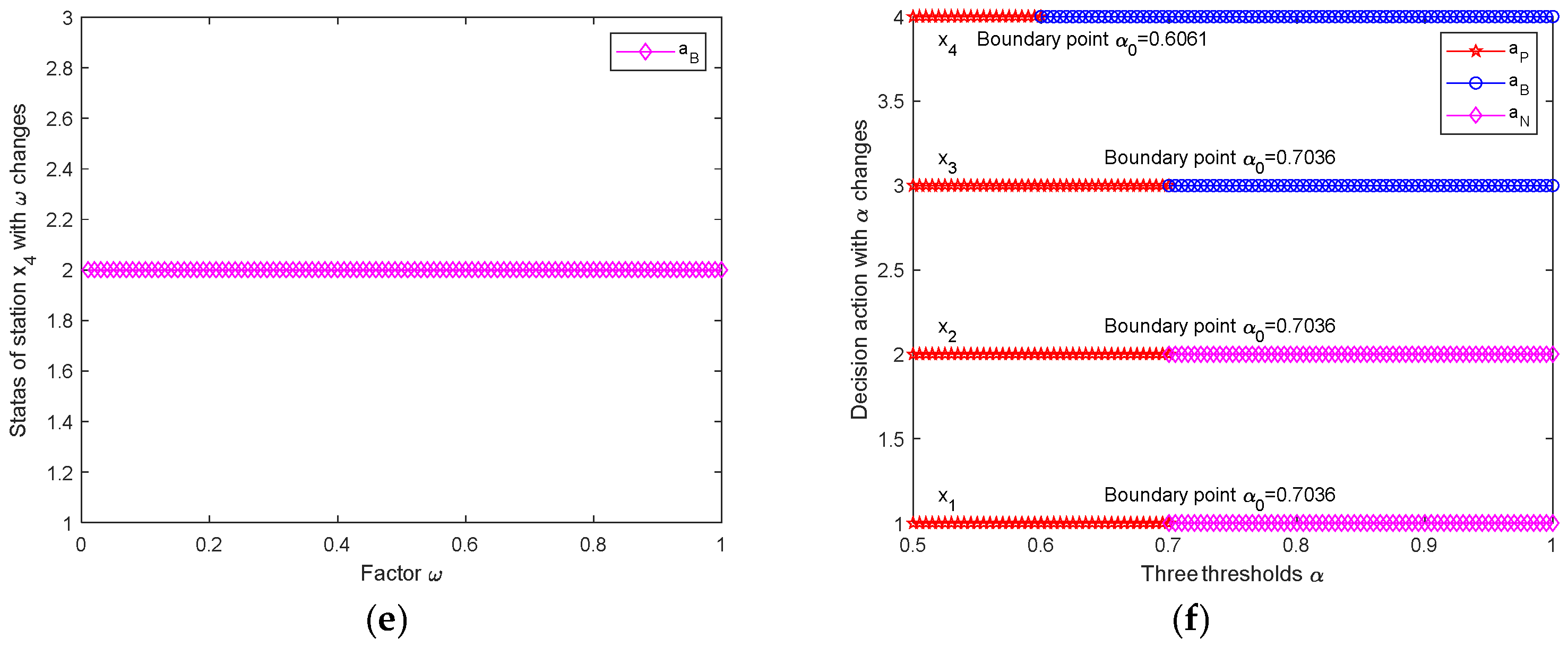
4.1. Result Analysis

To illustrate the effectiveness of the developed method,

Table 4. The emergency evacuation evaluation matrices.

	C1	C2	C3	C4	C5	Cd
x1	($\sqrt{0.8}$,$\sqrt{0.2}$)	($\sqrt{0.7}$,$\sqrt{0.3}$)	($\sqrt{0.6}$,$\sqrt{0.3}$)	($\sqrt{0.5}$,$\sqrt{0.5}$)	($\sqrt{0.7}$,$\sqrt{0.2}$)	($\sqrt{0.7}$,$\sqrt{0.3}$)
x2	($\sqrt{0.7}$,$\sqrt{0.2}$)	($\sqrt{0.6}$,$\sqrt{0.4}$)	($\sqrt{0.8}$,$\sqrt{0.2}$)	($\sqrt{0.7}$,$\sqrt{0.2}$)	($\sqrt{0.5}$,$\sqrt{0.5}$)	($\sqrt{0.6}$, $\sqrt{0.4}$)
x3	($\sqrt{0.6}$,$\sqrt{0.4}$)	($\sqrt{0.9}$,$\sqrt{0.1}$)	($\sqrt{0.8}$,$\sqrt{0.2}$)	($\sqrt{0.4}$,$\sqrt{0.6}$)	($\sqrt{0.7}$,$\sqrt{0.3}$)	($\sqrt{0.7}$,$\sqrt{0.3}$)
x4	($\sqrt{0.9}$,$\sqrt{0.1}$)	($\sqrt{0.5}$,$\sqrt{0.4}$)	($\sqrt{0.6}$,$\sqrt{0.3}$)	($\sqrt{0.7}$,$\sqrt{0.1}$)	($\sqrt{0.6}$,$\sqrt{0.4}$)	($\sqrt{0.8}$,$\sqrt{0.2}$)

shows the emergency evacuation evaluation matrices. There are four HSRSs that need to be evaluated, $X=\left\{x_1,x_2,x_3,x_4\right\}$. The attributes are guidance system (C₍₁₎, emergency exit (C₍₂₎, emergency route (C₍₃₎, emergency stairway (C₍₄₎ and emergency management (C₍₅₎. Otherwise, the decision attribute (C_d) represents the acceptability level of attributes. The values of each attribute are given by the experts in the form of PFNs based on their professional knowledge. Assume that there are three actions in the two states (HSRS risk unacceptable (P) and acceptable (N)): taking measures to eliminate risks (a_P), tracking attribute levels continuously (a_B) and taking no measures (a_N). The risk loss of the three actions is represented by PFNs and is shown in

Table 5. Pythagorean fuzzy loss function matrix.

	${\mathit{X}}_{\mathit{\alpha }}^{\mathit{\beta }}\left(\mathit{P}\right)$	$\neg {\mathit{X}}_{\mathit{\alpha }}^{\mathit{\beta }}\left(\mathit{N}\right)$
aP	($\sqrt{0.1}$,$\sqrt{0.9}$)	($\sqrt{0.9}$,$\sqrt{0.1}$)
aB	($\sqrt{0.3}$,$\sqrt{0.5}$)	($\sqrt{0.3}$,$\sqrt{0.6}$)
aN	($\sqrt{0.8}$,$\sqrt{0.2}$)	($\sqrt{0.1}$, $\sqrt{0.8}$)

.

Assume that the thresholds $\alpha =0.7$, $\beta =0.3$ and the factor $\omega =0.5$, the steps of the emergency evacuation evaluation process are as follows:

Step 1: calculate the Pythagorean fuzzy closeness measures $\vartheta \left(x_i,x_k\right)\left(i,k=1,2,3,4\right)$ between the two stations $x_i$ and $x_k$ related to the condition attribute set $B=\left\{c_1,c_2,c_3,c_4,c_5\right\}$ by Equation (20), and the results are

$\vartheta \left(x_1,x_1\right)=\left(1,0\right)$, $\vartheta \left(x_1,x_2\right)=\left(0.8388,0.4976\right)$, $\vartheta \left(x_1,x_3\right)=\left(0.8926,0.4486\right)$, $\vartheta \left(x_1,x_4\right)=\left(0.7785,0.5444\right)$, $\vartheta \left(x_2,x_2\right)=\left(1,0\right)$, $\vartheta \left(x_2,x_3\right)=\left(0.7750,0.5879\right)$, $\vartheta \left(x_2,x_4\right)=\left(0.8949,0.3855\right)$, $\vartheta \left(x_3,x_3\right)=\left(1,0\right)$, $\vartheta \left(x_3,x_4\right)=\left(0.7094,0.6280\right)$, $\vartheta \left(x_4,x_4\right)=\left(1,0\right)$.

Step 2: calculate the Pythagorean fuzzy similar category ${\vartheta }_{\alpha }^{\beta }\left(x_i\right)\left(i=1,2,3,4\right)$. The $\left(\alpha ,\beta \right)$-level cut set $X_{\alpha }^{\beta }$ under the Pythagorean fuzzy concept is calculated by Equation (8). Meanwhile, $\delta \left(x_i\right)=I\left(X_{\alpha }^{\beta },{\vartheta }_{\alpha }^{\beta }\left(x\right)\right)$.

${\vartheta }_{\alpha }^{\beta }\left(x_1\right)=\left\{x_1,x_2,x_3\right\}$, ${\vartheta }_{\alpha }^{\beta }\left(x_2\right)=\left\{x_1,x_2,x_4\right\}$, ${\vartheta }_{\alpha }^{\beta }\left(x_3\right)=\left\{x_1,x_3\right\}$, ${\vartheta }_{\alpha }^{\beta }\left(x_4\right)=\left\{x_2,x_4\right\}$, $X_{\alpha }^{\beta }=\left\{x_1,x_3,x_4\right\}$, $\delta \left(x_1\right)=2/3$, $\delta \left(x_2\right)=2/3$, $\delta \left(x_3\right)=1$, $\delta \left(x_4\right)=1/2$.

Step 3: calculate the thresholds $\overline{\alpha }=0.6489$, $\overline{\beta }=0.3312$, $\overline{\gamma }=0.5170$. Because $\overline{\alpha }>\overline{\beta }$, the decision-makers adopt a 3WD model. $\delta \left(x_1\right)>\overline{\alpha }$, $\delta \left(x_2\right)>\overline{\alpha }$, $\delta \left(x_3\right)>\overline{\alpha }$ and $\overline{\beta }<\delta \left(x_4\right)<\overline{\alpha }$. Therefore, the stations $x_1$, $x_2$ and $x_3$ have high risks and must take measures to eliminate risks, and $x_4$ is at risk and needs to be continuously observed.

Then, the relationships among the decision action, factor and threshold are shown in Figure 1, and we can draw the following conclusions:

(1) In Figure 1a, the threshold value $\overline{\alpha }$ increases and $\overline{\beta }$ decreases with the increase of factor $\omega$, indicating that the more optimistic the decision-maker is about the risks, the higher the requirement to take measures to eliminate the risks; and the more pessimistic the decision-maker is, the lower the requirement to take no measures, which is consistent with people’s cognition or intuition.

(2) From Figure 1b–e, with the increase of $\omega$, their decision-making actions will change stations $x_1$ and $x_2$ from tracking risks to taking some measures to eliminate risks. The risk critical point of change is 0.4090, while the decision-making actions of $x_3$ and $x_4$ remain unchanged.

(3) Considering that the performance is in two states of acceptance and unacceptability, assuming that $\alpha +\beta =1$, with the increase of $\alpha$, the decision-making actions of the stations $x_1$, $x_2$, $x_3$ and $x_4$ will change, as shown in Figure 1f. $x_1$ and $x_3$ will change from taking measures to eliminate risks to taking no measures, and $x_2$ changes from taking measures to eliminate risks to tracking risks, and the threshold change critical point of $\alpha$ is 0.7036. The critical point of the change of $\alpha$ for $x_4$ from taking measures to eliminate risks to tracking risks is 0.6061.

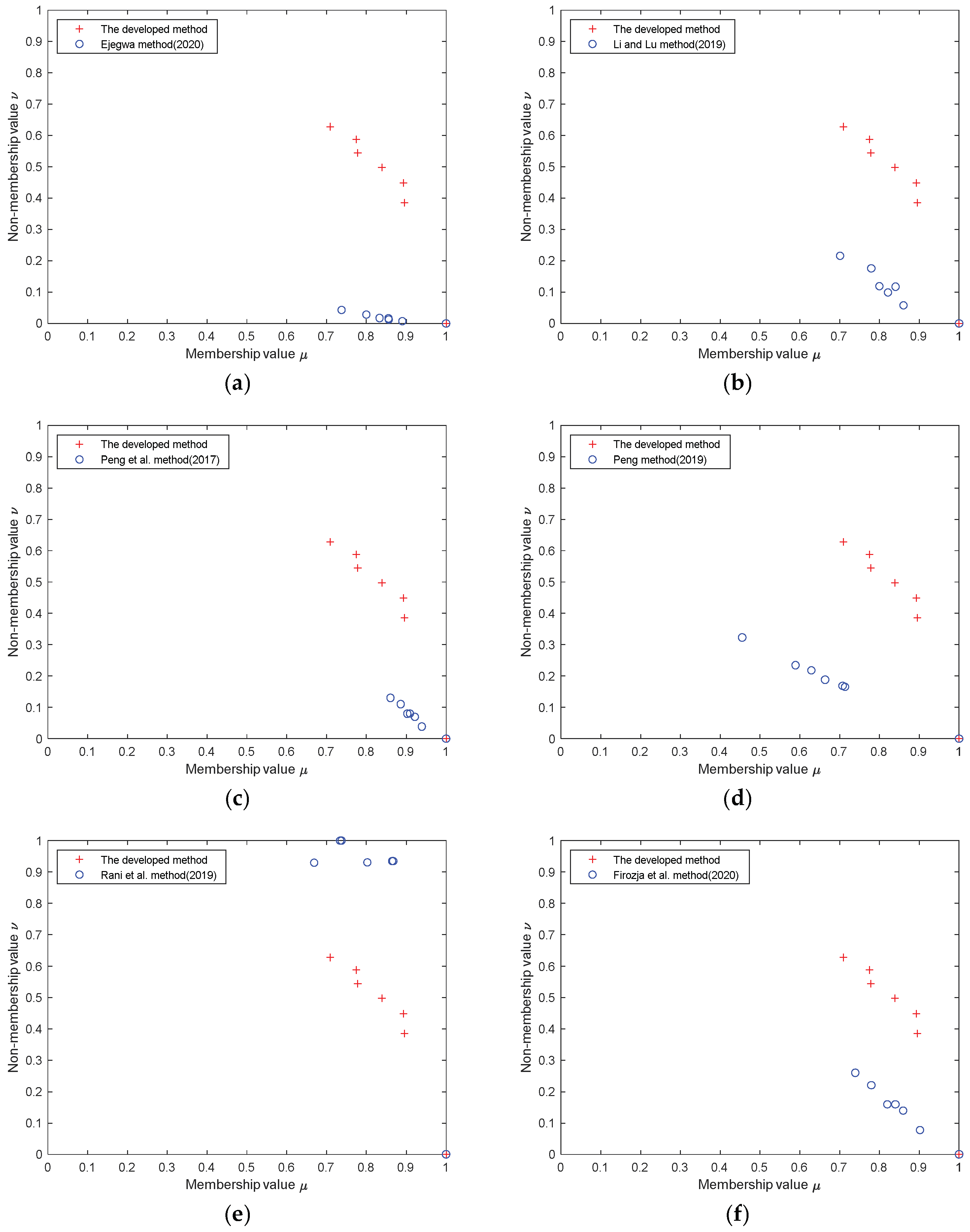
4.2. Comparison Analysis

To further illustrate the advantages of the developed Pythagorean fuzzy similarity, it is compared with the existing methods [33,34,35,36,39,40]. The obtained Pythagorean fuzzy closeness measure can be expressed by two-dimensional plane coordinates and the result is shown in Figure 2. The abscissa and ordinate are the membership degrees (μ) and non-membership degree (v) of the elements in the Pythagorean fuzzy similarity measure. Therefore, we can draw the following conclusions.

(1) Using different Pythagorean fuzzy similarity measure construction methods, the obtained Pythagorean fuzzy similarity measure will be different, which will have an impact on the final decision-making action of the stations $x_1$, $x_2$, $x_3$ and $x_4$. However, the existing six Pythagorean fuzzy similarity construction methods may be “against intuition” in some cases, and the developed Pythagorean fuzzy closeness measure can overcome these shortcomings of the existing similarity measures, as shown in Figure 2a–f.

(2) The developed Pythagorean fuzzy closeness measure takes significantly less time to calculate the similarity than the above six existing methods, especially the method of Li and Lu [33]. The proposed method constructs the closeness measurement in a single computational step, whereas other methods often require multiple iterations or calculations to achieve similar results [37].

(3) Most of the existing Pythagorean fuzzy similarity measures are based on the conditions that Pythagorean fuzzy similarity relations need to meet. In the construction process, the practical semantics of membership and non-membership are not considered. However, the constructed Pythagorean fuzzy closeness measure has the practical semantics of similarity and divergence measure.

5. Conclusions

A new Pythagorean fuzzy closeness measure was developed to overcome the shortcomings that the existing Pythagorean fuzzy similarity measures ignore the practical semantics of its membership and non-membership, and it may be “against intuition” in some cases. Then, it was introduced into a Pythagorean fuzzy decision system, and the concept of a Pythagorean fuzzy closeness measure and the $\left(\alpha ,\beta \right)$-cut set of two objects about conditional attribute sets were given, respectively. The $\left(\overline{\alpha },\overline{\beta }\right)$-lower approximation set of the Pythagorean fuzzy objective set and its positive domain, negative domain and boundary domain were derived by using rough membership degree as evaluation functions, and then the PF-3WD models with multi risk preferences were proposed according to Bayesian theory and applied to emergency evacuation evaluation. The results showed that the developed PF-3WD system deals with emergency evacuation evaluation effectively. Also, the developed Pythagorean fuzzy closeness measure overcomes the limitations of existing similarity measures by providing a more intuitive, computationally efficient, and semantically meaningful approach to decision-making in emergency evacuation scenarios.

The proposed model leverages Pythagorean fuzzy sets to combine quantitative data with qualitative judgments. This hybrid approach allows the model to effectively address the complexity and ambiguity of real-world evacuation problems, where purely quantitative data may be insufficient. Therefore, in future work, we will explore the systematic quantification of qualitative indicators, such as passenger behavior patterns, environmental factors, and expert judgments. This will involve developing standardized metrics for converting qualitative data into quantitative forms; validating these metrics through case studies and real-world applications; and integrating the quantified indicators into the PF-3WD model to further improve its accuracy and practicality.

References

1. Salarian, A.H.; Mashhadizadeh, A.; Bagheri, M. Simulating passenger evacuation in railway station under fire emergency using safe zone approach. Transp. Res. Rec. 2020, 2674, 806–812. [Google Scholar] [CrossRef]
2. Zhang, Z.; Yao, X.; Xing, Z.; Zhou, X. Understanding fire combustion characteristics and available safe egress time in underground metro trains: A simulation approach. Chaos Solitons Fractals 2024, 187, 115434. [Google Scholar] [CrossRef]
3. Zhang, Z.; Yao, X.; Xing, Z.; Zhou, X. Simulation on passenger evacuation of metro train fire in the tunnel. Chaos Solitons Fractals 2024, 187, 115429. [Google Scholar] [CrossRef]
4. Hassannayebi, E.; Memarpour, M.; Mardani, S.; Shakibayifar, M.; Bakhshayeshi, I.; Espahbod, S. A hybrid simulation model of passenger emergency evacuation under disruption scenarios: A case study of a large transfer railway station. J. Simul. 2020, 14, 204–228. [Google Scholar] [CrossRef]
5. Wan, J.; Sui, J.; Yu, H. Research on evacuation in the subway station in China based on the Combined Social Force Model. Phys. A Stat. Mech. Its Appl. 2014, 394, 33–46. [Google Scholar] [CrossRef]
6. Zhou, R.; Cui, Y.; Wang, Y.; Jiang, J. A modified social force model with different categories of pedestrians for subway station evacuation. Tunn. Undergr. Space Technol. 2021, 110, 103837. [Google Scholar] [CrossRef]
7. Zhou, Y.; Chen, J.; Zhong, M.; Hua, F.; Sui, J. Evacuation effect analysis of guidance strategies on subway station based on modified cellular automata model. Saf. Sci. 2023, 168, 106309. [Google Scholar] [CrossRef]
8. Wu, Y.; Kang, J.; Mu, J. Assessment and simulation of evacuation in large railway stations. Build. Simul. 2021, 14, 1553–1566. [Google Scholar] [CrossRef]
9. Zhang, J.; Huang, D.; You, Q.; Kang, J.; Shi, M.; Lang, X. Evaluation of emergency evacuation capacity of urban metro stations based on combined weights and TOPSIS-GRA method in intuitive fuzzy environment. Int. J. Disaster Risk Reduct. 2023, 95, 103864. [Google Scholar] [CrossRef]
10. Chen, J.; Liu, C.; Meng, Y.; Zhong, M. Multi-Dimensional evacuation risk evaluation in standard subway station. Saf. Sci. 2021, 142, 105392. [Google Scholar] [CrossRef]
11. Edrisi, A.; Lahoorpoor, B.; Lovreglio, R. Simulating metro station evacuation using three agent-based exit choice models. Case Stud. Transp. Policy 2021, 9, 1261–1272. [Google Scholar]
12. Zhang, Z.; Zhao, X.; Qin, Y.; Si, H.; Zhou, L. Interval type-2 fuzzy TOPSIS approach with utility theory for subway station operational risk evaluation. J. Ambient. Intell. Humaniz. Comput. 2022, 13, 1–15. [Google Scholar]
13. Zhang, Z.; Guo, J.; Zhang, H.; Zhou, L.; Wang, M. Product selection based on sentiment analysis of online reviews: An intuitionistic fuzzy TODIM method. Complex Intell. Syst. 2022, 8, 3349–3362. [Google Scholar]
14. Yao, Y. Three-way decisions with probabilistic rough sets. Inf. Sci. 2010, 180, 341–353. [Google Scholar]
15. Yao, Y. The superiority of three-way decisions in probabilistic rough set models. Inf. Sci. 2011, 181, 1080–1096. [Google Scholar]
16. Ma, W.; Lei, W.; Sun, B. Three-way group decisions under hesitant fuzzy linguistic environment for green supplier selection. Kybernetes 2020, 49, 2919–2945. [Google Scholar] [CrossRef]
17. Lei, W.; Ma, W.; Sun, B. Multigranulation behavioral three-way group decisions under hesitant fuzzy linguistic environment. Inf. Sci. 2020, 537, 91–115. [Google Scholar]
18. He, J.; Zhang, H.; Zhang, Z.; Zhang, J. Probabilistic linguistic three-way multi-attibute decision making for hidden property evaluation of judgment debtor. J. Math. 2021, 2021, 9941200. [Google Scholar]
19. Liang, D.; Liu, D. A novel risk decision making based on decision-theoretic rough sets under hesitant fuzzy information. IEEE Trans. Fuzzy Syst. 2014, 23, 237–247. [Google Scholar] [CrossRef]
20. Liang, D.; Pedrycz, W.; Liu, D.; Hu, P. Three-way decisions based on decision-theoretic rough sets under linguistic assessment with the aid of group decision making. Appl. Soft Comput. 2015, 29, 256–269. [Google Scholar]
21. Liang, D.; Liu, D. Systematic studies on three-way decisions with interval-valued decision-theoretic rough sets. Inf. Sci. 2014, 276, 186–203. [Google Scholar] [CrossRef]
22. Zhang, C.; Li, D.; Liang, J. Multi-granularity three-way decisions with adjustable hesitant fuzzy linguistic multigranulation decision-theoretic rough sets over two universes. Inf. Sci. 2020, 507, 665–683. [Google Scholar] [CrossRef]
23. Zhang, Z.; Zhang, H.; Zhou, L. Zero-carbon measure prioritization for sustainable freight transport using interval 2 tuple linguistic decision approaches. Appl. Soft Comput. 2023, 132, 109864. [Google Scholar] [CrossRef]
24. Sun, B.; Ma, W.; Li, B.; Li, X. Three-way decisions approach to multiple attribute group decision making with linguistic information-based decision-theoretic rough fuzzy set. Int. J. Approx. Reason. 2018, 93, 424–442. [Google Scholar] [CrossRef]
25. Zhang, X.; Chen, D.; Tsang, E.C. Generalized dominance rough set models for the dominance intuitionistic fuzzy information systems. Inf. Sci. 2017, 378, 1–25. [Google Scholar] [CrossRef]
26. Zhang, H.; Ma, Q. Three-way decisions with decision-theoretic rough sets based on Pythagorean fuzzy covering. Soft Comput. 2020, 24, 18671–18688. [Google Scholar] [CrossRef]
27. Zhang, S.P.; Sun, P.; Mi, J.S.; Feng, T. Belief function of Pythagorean fuzzy rough approximation space and its applications. Int. J. Approx. Reason. 2020, 119, 58–80. [Google Scholar] [CrossRef]
28. Zhang, Z.; Zhang, H.; Zhou, L.; Qin, Y.; Jia, L. Incomplete pythagorean fuzzy preference relation for subway station safety management during COVID-19 pandemic. Expert Syst. Appl. 2023, 216, 119445. [Google Scholar] [CrossRef]
29. Mandal, P.; Ranadive, A.S. Decision-theoretic rough sets under Pythagorean fuzzy information. Int. J. Intell. Syst. 2018, 33, 818–835. [Google Scholar] [CrossRef]
30. Liang, D.; Xu, Z.; Liu, D.; Wu, Y. Method for three-way decisions using ideal TOPSIS solutions at Pythagorean fuzzy information. Inf. Sci. 2018, 435, 282–295. [Google Scholar] [CrossRef]
31. Zhang, S.P.; Sun, P.; Mi, J.S.; Feng, T. Three-way Decision Models of Cognitive Computing in Pythagorean Fuzzy Environments. Cogn. Comput. 2021, 14, 2153–2168. [Google Scholar]
32. Wei, W.; Liang, J. Information fusion in rough set theory: An overview. Inf. Fusion 2019, 48, 107–118. [Google Scholar] [CrossRef]
33. Rani, P.; Mishra, A.R.; Pardasani, K.R.; Mardani, A.; Liao, H.; Streimikiene, D. A novel VIKOR approach based on entropy and divergence measures of Pythagorean fuzzy sets to evaluate renewable energy technologies in India. J. Clean. Prod. 2019, 238, 117936. [Google Scholar]
34. Peng, X.; Yuan, H.; Yang, Y. Pythagorean fuzzy information measures and their applications. Int. J. Intell. Syst. 2017, 32, 991–1029. [Google Scholar] [CrossRef]
35. Li, Z.; Lu, M. Some novel similarity and distance measures of pythagorean fuzzy sets and their applications. J. Intell. Fuzzy Syst. 2019, 37, 1781–1799. [Google Scholar]
36. Firozja, M.A.; Agheli, B.; Jamkhaneh, E.B. A new similarity measure for Pythagorean fuzzy sets. Complex Intell. Syst. 2020, 6, 67–74. [Google Scholar]
37. Li, P.; Wu, J.M.; Zhu, J.J. Stochastic multi-criteria decision-making methods based on new intuitionistic fuzzy distance. Syst. Eng.—Theory Pract. 2014, 36, 1517–1524. [Google Scholar]
38. Zhang, X. A novel approach based on similarity measure for Pythagorean fuzzy multiple criteria group decision making. Int. J. Intell. Syst. 2016, 31, 593–611. [Google Scholar]
39. Ejegwa, P.A. Distance and similarity measures for Pythagorean fuzzy sets. Granul. Comput. 2020, 5, 225–238. [Google Scholar]
40. Peng, X. New similarity measure and distance measure for Pythagorean fuzzy set. Complex Intell. Syst. 2019, 5, 101–111. [Google Scholar] [CrossRef]
Figure 1. The relationship between decision-making action, factor ω and the threshold α. (a) Changes of three thresholds; (b) Status change of station x1; (c) Status change of station x2; (d) Status change of station x3; (e) Status change of station x4; (f) Decision action changes.
Applsci 15 04087 g001aApplsci 15 04087 g001b
Figure 2. Comparative analysis between the developed Pythagorean fuzzy closeness measure and the existing methods. (a) Ejegwa’s method; (b) Li and Lu’s method; (c) Peng et al.’s method; (d) Peng’s method; (e) Rani et al.’s method; (f) Firozja et al.’s method.
Applsci 15 04087 g002