An Unsupervised Hybrid Approach for Detection of Damage with Autoencoder and One-Class Support Vector Machine

Abstract

Progressive deterioration and accumulated damage due to overloading, extreme events, and fatigue necessitate the continuous monitoring of civil infrastructure to ensure serviceability and safety. With advances in sensor technology, data-driven structural health monitoring (SHM) strategies, particularly artificial neural networks (ANNs), have gained prominence for analyzing large datasets and identifying complex patterns. Among these, autoencoders (AEs), a specialized class of ANNs, are well-suited for unsupervised learning tasks, enabling dimensionality reduction and feature extraction. This study employs transmissibility functions (TFs) as training samples for the AE. TFs are directly derived from response measurements without the need to measure input and exhibit local sensitivity to changes in dynamic properties, making them an efficient feature for structural assessment. The reconstruction errors in TFs, quantifying the deviation between the original and AE-reconstructed data, are leveraged as damage-sensitive features for classification using a one-class support vector machine (OC-SVM). The proposed methodology is validated through numerical simulations with noise-contaminated data representing various damage scenarios in a shear-building model, as well as experimental tests on a masonry arch bridge model subjected to progressive damage. Numerical investigations demonstrate improved detection accuracy and robustness of the procedure through the incorporation of nonlinear encoding into the dimensionality reduction process, compared to the classical principal component analysis method.. Experimental results confirm the framework’s effectiveness in detecting and localizing damage using unlabeled field data.

1. Introduction

Structural degradation in civil infrastructure, driven by factors such as excessive loading, environmental stressors, and material fatigue, highlights the need for continuous monitoring to maintain safety and functionality. Limitations in traditional visual inspections, such as shortage of qualified labor and inaccessibility to critical structural components, have led to the development of vibration-based SHM techniques for assessing structural conditions. In recent years, the research in this field has increasingly focused on intelligent applications utilizing data-driven methods that do not require physical models [1]. This approach is often regarded as a statistical pattern recognition paradigm, involving the extraction of damage sensitive features from the acquired data and classification of the extracted features utilizing statistical modeling. In this framework, a significant challenge is that for most structural systems, only data from the baseline or current state are available. Considering the countless potential damage scenarios that can arise, ‘unsupervised’ approaches—which learn solely from the data representing the healthy condition while accounting for operational and environmental variability—are essential for classification [2,3,4,5]. Given the challenges associated with measuring input excitation during data acquisition, output-only approaches relying only on vibration response measurements, emerge as more suitable for civil engineering applications [6,7,8].

In this regard, a number of machine learning and statistical inference techniques have been implemented to health monitoring applications. Artificial neural networks (ANNs) based on machine learning provide such a computational approach that can be applied to systems where large volumes of data are available and complex patterns need to be identified for analysis and prediction of these data. Among these, autoencoders (AEs) are a specialized class of ANNs, mainly designed for unsupervised learning, with the purpose of dimensionality reduction and feature learning [9].

An AE consists of two main components: an encoder and a decoder. The encoder maps high-dimensional input data into a lower-dimensional latent space, capturing essential features while discarding redundant information. The decoder then reconstructs the original input from this compressed representation, aiming to minimize the reconstruction error. This process enables AEs to learn intrinsic structures within the data, making them particularly valuable for anomaly detection, denoising, and representation learning. In anomaly detection tasks, AEs are trained to minimize reconstruction error only on normal data instances, thus involving high reconstruction error on anomalous data. Then, the reconstruction error is exploited to classify the input data.

AEs demonstrate remarkable flexibility, enabling customization for various data types and tasks through adjustments to their architecture or objective functions. Various AE architectures have been proposed to address specific challenges and enhance performance across different domains, categorized by network structure as follows: standard, regularization-based, generative, convolutional, recurrent, semi-supervised, graph-based, robust, and masked AEs [10]. For example, convolutional AEs are commonly used in image processing tasks, while recurrent AEs excel in handling sequential data. Generative AEs focus on learning the underlying probability distribution of data rather than solely performing dimensionality reduction. Variational AEs, a subtype of generative AEs, are designed to generate new data samples and improve model generalization. With each architecture having its own advantages and limitations, specific requirements of the application domain have to be considered in selecting an appropriate architecture.

The capacity of the AEs to model complex patterns and detect anomalies that are not easily identifiable makes them well-suited for vibration-based SHM applications. Over the past few years, a growing body of research has focused on exploiting this capability for SHM in civil engineering systems. Various studies have advanced this field, each contributing to the different aspects of AE application. Pathirage et al. [11] proposed an AE-based deep-learning framework to model the relationship between the structural vibration characteristics and the physical properties of the structure. Similarly, Anaissi et al. [12] employed energy levels of standardized time series data as the inputs of an AE to monitor the health state of a bridge and a three-story building. Lee et al. [13] developed a convolution AE-based novelty detection approach for detecting tendon damage in prestressed concrete bridges. Ma et al. [14] applied a variational auto encoder technique to the damage identification of a beam-like bridge subjected to a moving vehicle and validated their methodology through both numerically simulated and experimental data. Yan et al. [15] presented a multi-domain indicator-based optimized stacked deep AE to perform fault identification of rolling bearings. Rastin et al. [16] proposed an unsupervised deep learning-based method for structural damage detection based on convolutional AEs that employs acceleration signals from the structure and is trained by the signals solely acquired from the healthy state of the structure. Wang and Cha [17] employed a deep AE to extract damage-sensitive features from measured acceleration response data of a healthy structure. These features were then used by a one-class support vector machine for damage detection. Lee et al. [18] demonstrated the effectiveness of a convolutional auto encoder-based methodology for detecting damage using the acceleration and strain data from field experiments on an actual bridge structure. Jiang et al. [19] proposed an approach that employs two deep AEs: an undercomplete AE in the latent domain to capture the low-dimensional manifold of the signal and an overcomplete AE in the time domain to extract reconstruction error-based damage indicators. Silva et al. [20] proposed a stacked AE approach that uses modal parameters extracted from measured vibration data as input as the first level features used to train the stacked auto encoder to perform a second-level feature extraction from the bottleneck layer as the damage-sensitive features. Shang et al. [21] used a deep convolutional denoising AE-based strategy to reconstruct cross correlations of the vibration data extracting the desired features and identifying minor damage through the control charts established for these features. Zhang et al. [22] exploited a convolutional variational auto-encoder for tunnel damage detection, employing wavelet packet energy to pinpoint damage locations. Spinola Neto et al. [23] investigated the effectiveness of four AE-based methodologies—conventional, sparse, variational, and convolutional—across three different test structures. Using a statistical tool to analyze damage detection and progression, reflected by an increase in the quantified reconstruction error, the study found that the variational AE demonstrated superior performance compared to the other methods. Römgens et al. [24] highlighted the suitability of AEs trained with time series data for damage localization under ambient conditions. In the frequency domain, an unsupervised deep AE model was trained on the response of a vehicle passing a healthy bridge, and the effectiveness of a damage index—based on the difference between the original and reconstructed responses—was explored [25]. Li et al. [26] proposed a generalized AE approach integrated with a statistical pattern recognition strategy, utilizing power cepstral coefficients of structural acceleration responses as damage-sensitive features for structural damage assessment. Lin et al. [27] constructed a variational AE network model for detecting bridge damage utilizing response data from limited sensors. In the time-frequency domain, a deep convolutional AE model was proposed to utilize wavelet transmissibility pattern spectra as input data for characterizing damage information, combined with an unsupervised clustering algorithm for damage classification [28].

The success of these varied approaches to SHM largely depends on how well the AE can capture and reconstruct key features from the input data as accurately as possible by encoding them. To enhance the accuracy of this encoding, input data must be carefully selected to ensure effective representation of the information. Resende et al. [29] have shown that compressions and reconstructions performed by the AEs were more accurate in the frequency domain compared to the time domain since a Fourier transformation algorithm serves as an initial parameter extractor that facilitates this encoding.

Another critical factor for the reliability of these approaches is the quality and usefulness of the collected data. The effectiveness of the monitoring system depends not only on data processing techniques but also on optimal sensor placement, which influences the accuracy of the acquired information [30,31]. Strategic sensor placement—both in terms of number and distribution—ensures that critical structural behaviors are captured, the signal-to-noise ratio is optimized, and meaningful changes in the structural response can be detected. Moreover, considering the structural topology when deploying sensors enhances the damage localization capabilities, further improving the robustness of the monitoring system [32,33].

In this context, the transmissibility function (TF) stands out as a promising candidate to be processed as the input to be reconstructed by the AE. Transmissibility is a frequency-domain representation that relates the output response at one measurement point to the response at another, independent of excitation measurements. This characteristic makes it particularly suitable for SHM, as it enables damage detection by capturing localized changes in dynamic properties. The concept of transmissibility for damage detection has been explored extensively. A critical review on the use of TFs for damage detection and localization from an analytical standpoint is presented by Chesne and Deraemaeker [34]. Li et al. [35] developed the power spectral density transmissibility concept for response reconstruction and damage identification within the model-update framework. Zhu et al. [36] explored the damage sensitivities of TFs on a lumped mass model in their research, using inversion of a tri-diagonal matrix. The following study by Zhou et al. [37] developed a methodology utilizing TFs in conjunction with principal component analysis (PCA) and validated the approach on both numerically simulated data and experimental data. Yan et al. [38] provided a comprehensive review on the fundamentals of TFs as a mathematical representation of output-to-output relationships as well as TF-based system identification and damage detection. Liu et al. [39] employed TFs with one-dimensional convolutional neural networks in a deep learning strategy. Lei et al. [40] proposed an approach for detecting structural damage subject to unknown seismic excitation with wavelet-based transmissibility of structural response data utilized as inputs to the pre-trained convolutional neural network.

Despite extensive research on damage detection using machine learning, several challenges remain unaddressed. In particular, the effectiveness of AE-based methods is often hindered by the nature of the input data, reliance on subjective thresholding, and the need for labeled datasets in supervised approaches. Additionally, many studies focus on detecting damage but do not explicitly address localization. To contextualize the contributions of this study, key research gaps are outlined below:

• Many studies use raw vibration signals as inputs to AE models. However, raw vibration data are high-dimensional and complex due to noise contamination, high-frequency content, and abrupt waveform variations [41]. These characteristics complicate feature extraction in unsupervised learning due to the lack of labeled guidance.
• The discrete nature of raw vibration data or their low-level features can degrade training efficiency and fitting accuracy [42]. To address this, deep AE architectures are often employed; however, they introduce a large number of parameters requiring optimization, which increases computational cost and the risk of overfitting.
• Many unsupervised learning-based methods rely on manually defined damage thresholds based on reconstruction loss. This subjectivity can lead to inconsistent damage detection outcomes.
• Most studies focus on detecting damage and assessing its severity in a comparative manner but do not explicitly address spatial localization, limiting their practical application in SHM.
• While many damage detection methods are validated solely through numerical examples, experimental validation on physical structures remains limited.

To address these challenges, this study proposes an unsupervised damage detection framework that integrates transmissibility-based features with an AE and an OC-SVM for automated damage identification and localization. In the first step, the auto-encoder is trained on the measured local TFs from the baseline (healthy) state. The learned representation is then utilized to reconstruct the measured TFs for an unknown health state. Based on the deviations between the reconstructed output from that of the measured, specifically the reconstruction error, the OC-SVM classifier is utilized for classifying damaged states as anomalies. This detection stage is augmented by a localization approach that fuses data from all sensors in the final stage.

The major contributions of this study are as follows:

• The proposed methodology utilizes local TFs derived directly from response measurements in the frequency domain, reducing the computational burden associated with time-domain data. Additionally, it eliminates the need for preprocessing steps such as natural frequency and mode shape extraction, along with the errors introduced by frequency-domain feature selection.
• The proposed framework integrates an AE with an OC-SVM, requiring only baseline-state training data for damage detection. This eliminates the need for labeled datasets and supervised learning, making the approach suitable for monitoring civil engineering structures where damage-state data are either unavailable or difficult to obtain.
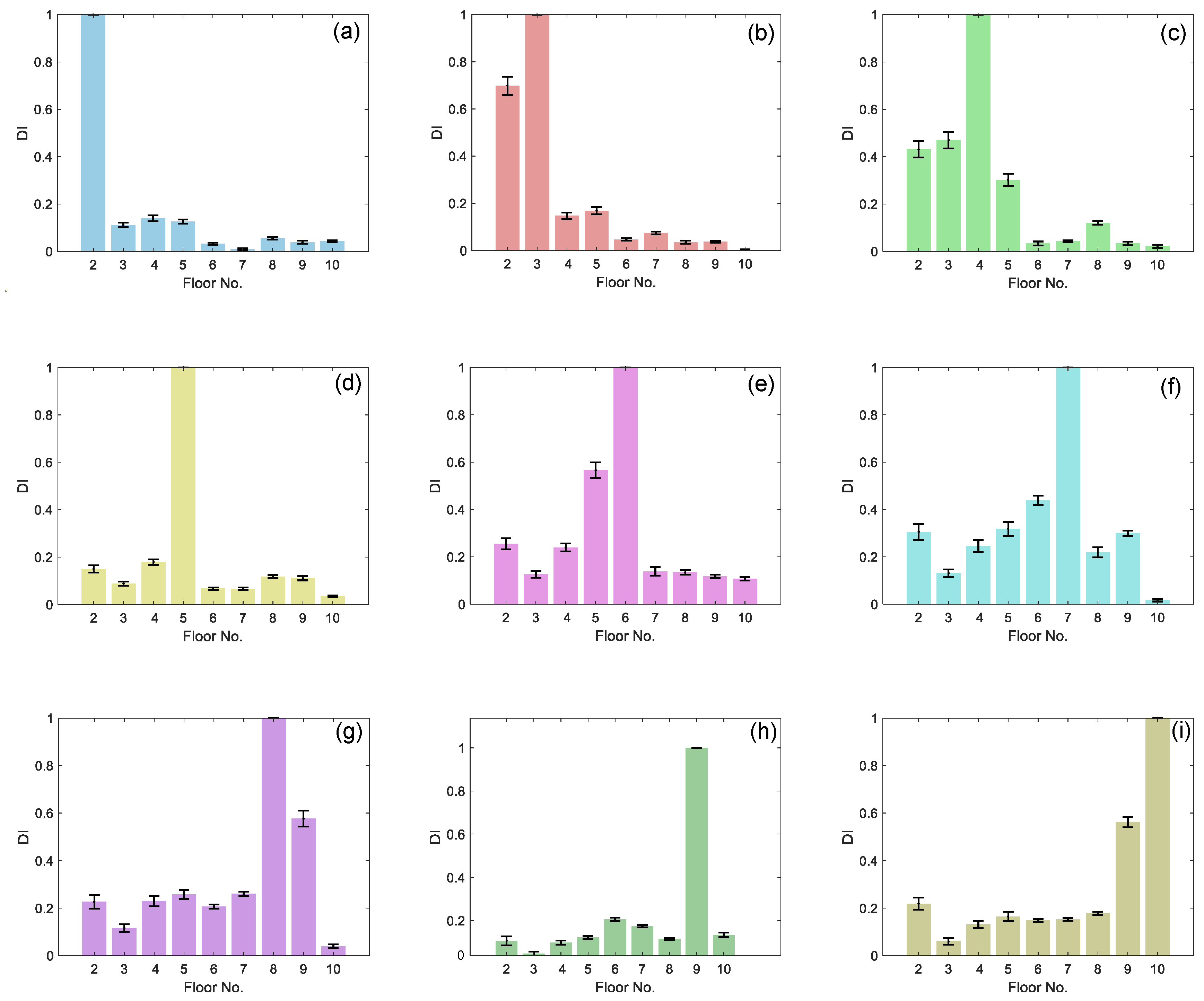
• A novel damage index is proposed, enabling the spatial localization of damage within the resolution of the sensor network.
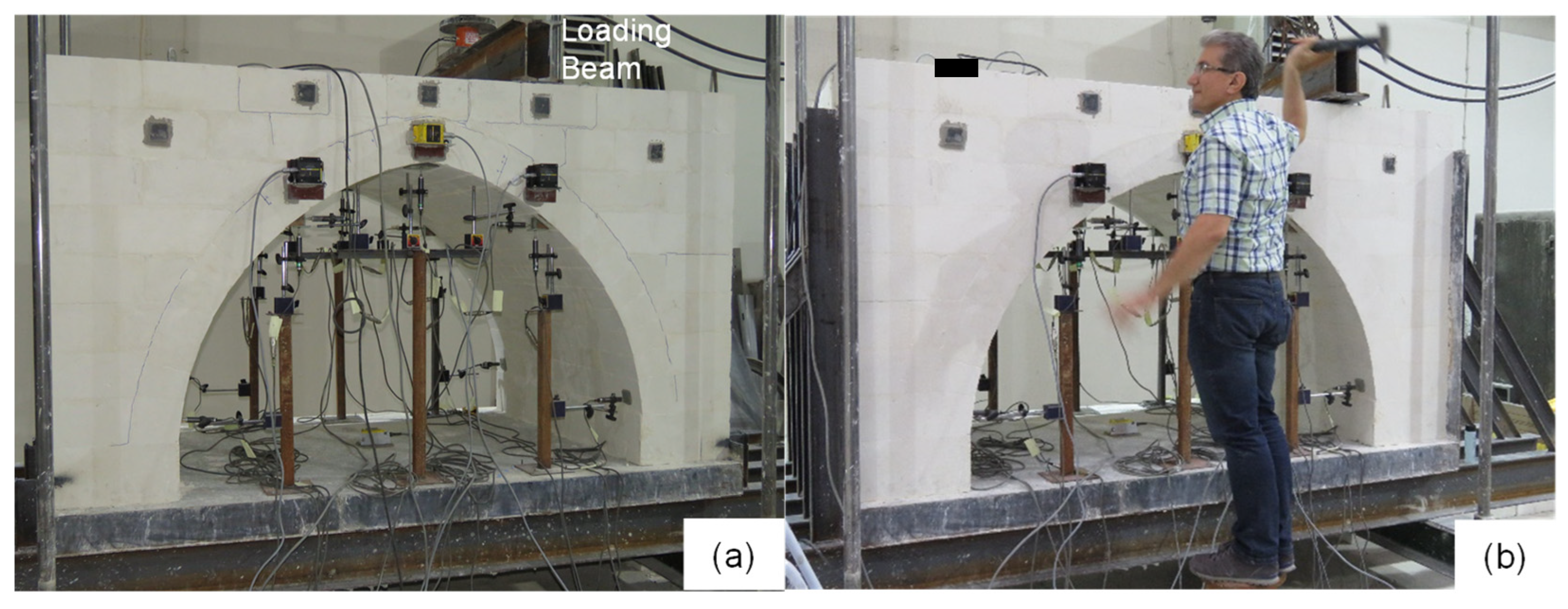
• The methodology is validated using experimental data from a scaled model of an arch bridge, demonstrating its applicability in real-world scenarios beyond numerical simulations.

The remainder of this paper is organized as follows. First, the two-step feature extraction and damage detection localization methodology is introduced. The employed AE-based framework for feature extraction and the OC-SVM classifier to detect damage with the extracted features is discussed next. The numerical simulations demonstrating the performance of the AE by fine tuning the hyperparameters including the activation function, the number of hidden layer neurons and the number of epochs is followed by the presentation of the experimental work on a 1/4-scaled arch bridge to evaluate the proposed damage detection method. This paper concludes with a discussion of the results and the final remarks on the conclusions drawn.

2. Research Methodology

The two-stage damage identification framework presented in this paper integrates an AE for reconstructing the measured TF and an OC-SVM for interrogating the reconstruction errors. The general structure of this hybrid approach is illustrated in Figure 1. The AE-based framework is trained on the TFs obtained from the measured acceleration data. The reconstruction error from this learned representation is then fed into the OC-SVM to train the algorithm for detecting damage. Once this training is completed with the data from the baseline state of the system, data collected from an unknown state can be tested for monitoring structural health.

Expanding on this framework, Section 2.1 introduces the local TFs obtained between two sensor locations, Section 2.2 provides a brief overview of the traditional AE implemented for this purpose, and Section 2.3 summarizes the concept of OC-SVM and outlines the specifics of the implemented machine for detecting damaged state. The procedure to fuse the sensor information for localizing the damaged region is described in Section 2.4.

2.1. Transmissibility as Damage Sensitive Feature

The local transmissibility between the two coordinates i and j, with reference to input location k, can be defined in the frequency domain as the ratio of two responses X_i and X_j, directly as follows:

$$T_{ij}^k\left(\omega \right)={\displaystyle \frac{X_i\left(\omega \right)}{X_j\left(\omega \right)}}$$

(1)

Due to its inherent relationship with structural properties, changes in these properties are reflected in the TF, making it a salient damage-sensitive feature for monitoring structural health [43]. Furthermore, because it characterizes the vibration response across small sections of the structure, the TF is expected to be particularly sensitive to localized damage. The local TF, obtained using Equation (1), eliminates the need for direct measurement of the input; however, it requires impact testing across multiple locations to generate a comprehensive set of TFs.

Among possible loading (unmeasured) conditions that can be implemented for damage detection purposes, a potential alternative with practical significance is to use a single input moved to different points on the structure. For each excitation location, a transmissibility matrix of size $N\times N$, elements of which are functions of frequency can be formed for all combinations of outputs between location pairs. The selection of appropriate ones as damage detection features is essential not only for reducing the dimensionality of the original dataset but for eliminating the unrelated variables to ensure the success of the proposed methodology. To ‘close-in’ the damaged region, typically the two successive pairs of coordinates are selected and the transmissibility corresponding to the two adjacent coordinates along the structure are interrogated. This corresponds to the first-upper diagonal of the matrix with entries of $T_{12}, T_{23},\dots T_{k,k+1}$. Furthermore, to limit the dependence of the TF outside the domain enclosed by the output coordinates, the input location is also arranged such that it is collocated with one of the output coordinates. Hence, with these two criteria imposed on the selection, the number of TFs retained as damage detection features reduces down to $N-1$ to for an N-DOF system. With input location indicated as the superscript, the vector of selected features for damage detection as a function of frequency are defined as $T_{12}^2,T_{23}^3, \cdots T_{k,k+1}^{k+1},\dots T_{N-1,N}^N$.

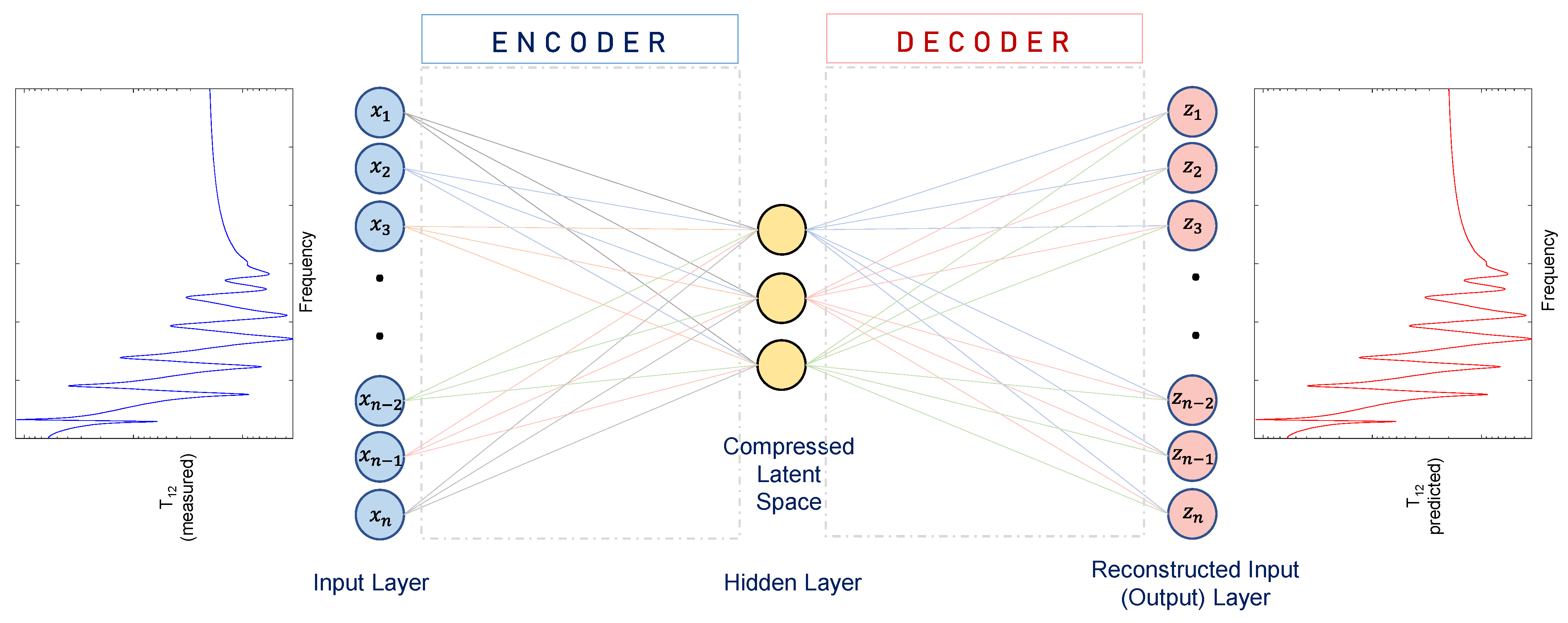
2.2. Autoencoder Architecture

An AE is an unsupervised feedforward neural network designed to match its output values with its input values through repeated application of backpropagation to minimize the reconstruction error between the input and output [10]. A typical AE consists of three parts: an input layer, one or more hidden layers, and an output (reconstructed input) layer. The hidden layer is composed of two key components: the encoder and the decoder. The encoder at the hidden layer compresses the input data into a lower-dimensional space by extracting and encoding its most significant features. The decoder then reconstructs the original input from this compressed representation using various reconstruction techniques, ensuring the generated outputs closely resemble the inputs. To facilitate accurate data reconstruction, the output layer is the same size as the input layer. This ensures that the algorithm learns the compressed representations used to approximate input data and not just the identity function which remembers the original input.

Figure 2 presents the typical architecture of an undercomplete AE, that features a single hidden layer with fewer neurons than the input layer (bottleneck), forcing the AE to learn a compressed representation of the input data. The encoder f(x), transforming an n-dimensional input $x\in {\mathfrak{R}}^n$ to an r-dimensional representation h$\in {\mathfrak{R}}^r$ (r < n), at the hidden layer, capturing the most important features of the input data, can be expressed as follows:

$$f\left(x\right)=h=\Phi (Wx+b)$$

(2)

where $\Phi$ denotes the activation function; $W\in {\mathfrak{R}}^{r\times n}$ is the weight matrix of the encoder; and $b\in {\mathfrak{R}}^r$ is the bias vector for the input. The activation function is usually selected as a nonlinear function in the form of a sigmoid or hyperbolic tangent function.

The decoder g(h), transforming the compressed latent representation back into reconstructed vector z$\in {\mathfrak{R}}^n$, can be expressed as follows:

$$g\left(h\right)=g\left(f\left(x\right)\right)=z=\Phi (\widehat{W}h+\widehat{b})$$

(3)

where $\widehat{W}\in {\mathfrak{R}}^{n\times r}$ is the weight matrix of the decoder and $\widehat{b}\in {\mathfrak{R}}^n$ is the bias vector for the hidden layer.

During training, the AE is designed to learn a compact representation in the hidden layer by minimizing the difference between the original input and its reconstructed version using a mean squared error (MSE) loss function:

$$L\left(x,z\right)={‖x-z‖}_2^2$$

(4)

If the input is completely random, the compression task becomes challenging, requiring a large number of hidden units. To address this, a sparsity constraint is often imposed on the activations in the hidden layer. This encourages the AE to produce a more compact and sparse representation of the input data.

2.3. One-Class Support Vector Machine (OC-SVM)

The OC-SVM is an unsupervised classifier used for anomaly detection and outlier identification in datasets [44]. The objective of the OC-SVM is to learn a decision boundary that separates the majority of data points representing normal observations from the origin in a higher-dimensional feature space. This boundary is defined by a hyperplane that maximizes the margin between the data points and the origin, effectively creating a region where normal data points lie, while leaving anomalies or outliers outside of this region. The decision function, $f\left(x\right)$ is expressed as follows:

$$f\left(x\right)=w^T\varphi \left(x\right)-\rho$$

(5)

where $\varphi$(·) is a feature projection function that maps an input vector x into a higher dimensional feature space; $w$ is the decision hyperplane normal vector; and ρ is the bias term. They can be obtained by solving the following objective function:

$$\underset{\mathrm{w},\xi ,\rho }{\min }{\displaystyle \frac{1}{2}}{‖w‖}^2+{\displaystyle \frac{1}{\nu m}}\sum _{i=1}^m{\xi }_i-\rho$$

(6)

$$\begin{array}{c}\mathrm{subject} \mathrm{to}\\ w^T\varphi \left(x_i\right)\ge \rho -{\xi }_i, {\xi }_i>0, i=1, 2, \dots ,m\end{array}$$

(7)

where x_i are the training examples belonging to one class; $\nu \in (0, 1]$ determines the upper bound on the fraction of outliers and the lower bound on the number of training samples used as support vectors; and ${\xi }_i$ are non-zero slack variables for penalizing the outliers.

The feature mapping $\varphi (·)$ which can become computationally inefficient, especially for high dimensional data, can be replaced by a kernel function $K\left(x_i,x_j\right).$ By implicitly computing the inner product ${\varphi \left(x_i\right)}^T\varphi \left(x_j\right)$ in the feature space, this function eliminates the need for explicit feature mappings while ensuring computational efficiency and guaranteeing the existence of solutions [45]. Among the available kernels, the Gaussian kernel is a commonly chosen option due to its flexibility and effectiveness. It is expressed as follows:

$$K(x_i,x_j),=exp (-{\displaystyle \frac{{\parallel x_i-x_j\parallel }^2}{{2\sigma }^2}})$$

(8)

where $\sigma$ is the width of the Gaussian kernel.

2.4. Damage Localization

Damage detection using the OC-SVM is followed by localization estimation, achieved by comparing the differences between the measured and reconstructed transmissibilities for adjacent sensor locations $(i,j)$ distributed throughout the structure. This comparison is performed at each frequency increment ($f_k$) where the local transmissibilities are calculated, identifying the sensor pair with the largest discrepancy $(i^{\ast },j^{\ast })$:

$$({i^{\ast },j^{\ast })}_{f_k}=\underset{(i,j)}{\mathit{argmax}} △T_{ij}\left(f_k\right)$$

(9)

Once the individual maximums are identified across all frequency lines, the sensor pair with the maximum number of occurrences over the entire frequency range ${(i^{\ast },j^{\ast })}_{max}$, can be determined as the potential damage location:

$${(i^{\ast },j^{\ast })}_{max}=\underset{(i,j)}{\mathit{argmax}} N_{ij}$$

(10)

where N_ij is the number of times each sensor pair $(i,j)$ appears as ${(i^{\ast },j^{\ast })}_{f_k}$ over the entire frequency range $\left[f_1, f_2,\dots ,f_n\right]$. Based on the number of counts of maximum occurrences, a relative damage index indicating the sensor pair most likely associated with the damage location, and serving as a clear and comparable metric is expressed as follows:

$${DI}_{i,j}={\displaystyle \frac{N_{ij}}{N_{max}}}$$

(11)

where $N_{max}$ is the largest occurrence count across all sensor pairs.

3. Performance Evaluation

3.1. Simulation Study

The performance of the proposed damage identification methodology was first illustrated through numerical simulations carried out on a ten-story shear building model with sensor locations along with a non-uniform distribution of floor masses (m) and story stiffnesses (k), as shown in Figure 3. Damping ratio was assumed to be proportional and assigned as 2% for all modes. Damage scenarios included 10% loss of floor stiffness in each floor, one at a time. The analytically computed natural frequencies for the undamaged as well as the damaged cases are listed in

Table 1. Analytically computed natural frequencies (Hz) and percent changes relative to the baseline state.

	Natural Frequency (Hz)
	Mode 1	Mode 2	Mode 3	Mode 4	Mode 5	Mode 6	Mode 7	Mode 8	Mode 9	Mode 10
Baseline	1.45	3.75	6.07	8.22	10.08	11.96	13.24	14.40	15.05	16.25
D. Case 1	1.42	3.67	6.03	8.20	10.07	11.71	13.02	14.17	15.02	16.25
D. Case 2	1.42	3.72	6.07	8.08	9.88	11.89	13.18	13.99	14.98	16.24
D. Case 3	1.43	3.75	6.00	8.02	10.08	11.63	13.17	14.21	14.92	16.23
D. Case 4	1.43	3.73	5.94	8.22	9.84	11.96	12.97	14.40	14.83	16.15
D. Case 5	1.43	3.70	6.02	8.12	10.06	11.76	13.18	14.26	14.87	15.95
D. Case 6	1.44	3.68	6.07	8.08	9.92	11.96	13.04	14.30	15.05	15.80
D. Case 7	1.44	3.68	6.00	8.21	9.92	11.76	13.07	14.40	14.87	15.96
D. Case 8	1.45	3.70	5.89	8.11	10.03	11.96	13.15	14.17	14.80	16.15
D. Case 9	1.45	3.73	5.98	8.10	9.91	11.80	12.95	14.23	14.90	16.21
Percent change (%)
	Mode 1	Mode 2	Mode 3	Mode 4	Mode 5	Mode 6	Mode 7	Mode 8	Mode 9	Mode 10
D. Case 1	2.44	2.07	0.74	0.24	0.09	2.06	1.60	1.61	0.21	0.01
D. Case 2	2.18	0.82	0.02	1.72	1.98	0.55	0.43	2.84	0.49	0.03
D. Case 3	1.80	0.02	1.25	2.45	0.02	2.71	0.49	1.32	0.85	0.13
D. Case 4	1.68	0.57	2.25	0.01	2.42	0.00	2.04	0.00	1.45	0.62
D. Case 5	1.27	1.45	0.85	1.21	0.22	1.66	0.40	0.97	1.20	1.86
D. Case 6	0.84	2.00	0.02	1.67	1.63	0.00	1.45	0.66	0.00	2.78
D. Case 7	0.46	1.86	1.27	0.05	1.58	1.64	1.22	0.01	1.21	1.77
D. Case 8	0.24	1.45	3.10	1.29	0.48	0.00	0.65	1.57	1.67	0.62
D. Case 9	0.06	0.45	1.55	1.40	1.70	1.36	2.20	1.13	1.01	0.21

.

Data for the baseline state, necessary for initial training and subsequent testing, were generated using the finite element model of the frame by assigning an initial velocity at each sensor location, one at a time. Acceleration measurements were simulated at these positions with a sampling time of 0.01 s. over a 60 s period and these data were then contaminated with varying levels of noise, randomly distributed within the range of 2% to 5%. The resulting signal pool included 60 sets of acceleration measurements utilized to compute the TFs. From this baseline data pool, the first 40 were used to train the classification model, while the remaining 20 were reserved for validation.

Damage states for testing were simulated by introducing a 20% reduction in the story stiffness at each floor, one at a time. This resulted in nine damage scenarios, each representing single-floor damage. For each damage scenario, 20 sets of acceleration data were generated following the same procedure and noise contamination levels. TFs were then calculated from these datasets to be tested with the trained model.

The next stage involved training a conventional undercomplete AE using only the baseline dataset, to learn a compact representation of the transmissibility by first compressing it to a lower-dimensional space and then reconstructing it from this representation. A key element in training the AE is the number of neurons in the hidden layer, as it directly determines the size of the compact representation, or latent space, in this single, hidden layer AE. The optimal number of neurons should fit the training data well while maintaining the capability to generalize to new and unseen data.

To determine the optimal architecture, Figure 4 displays the MSE for each TF across different neuron counts. The number of epochs in these plots is a hyperparameter to be selected based on the performance of the model. An epoch represents one cycle of training where the model learns from the data and updates its weights. Multiple epochs are often needed since the model may not fully learn the data in a single pass. However, an excessive number of epochs may lead the model to overfit its training data since it indicates that the model is memorizing the data rather than learning it.

Figure 5 compares the MSE of the training and the validation (unseen) data for n = 3 neurons. This value is found to be optimal with the number of epochs set to 20, since it ensures that the model captures the underlying structure of the transmissibility data without compromising performance on unseen cases.

With the selected architecture, the 512 dimensional input data were compressed into a three-dimensional latent space while preserving the most significant features of the input transmissibility data. Since transmissibility, defined as the ratio of amplitudes across different frequencies, is a positive-valued function, a log-sigmoid activation function was employed for the encoder for an effective mapping of the input to a constrained range. For the decoder, however, a linear transfer function was employed for the accurate reconstruction of the input data. The training of the AE is based on minimizing the reconstruction error, calculated as the MSE between the input and output vectors and the network weights are adjusted through backpropagation, with gradients computed using stochastic gradient descent. In this process, each TF was treated as an independent input and trained separately.

To assess the AE’s effectiveness in capturing the data structure and mitigating measurement noise, its performance was compared to PCA, a linear dimensionality reduction technique that projects the data onto a subspace defined by the principal components. In PCA-based data compression, the projection P, of the input transmissibility T is given as follows:

$$P=UT$$

(12)

where U represents the principal components obtained from the eigenvectors of the covariance matrix of the transmissibility data.

For consistency with the AE’s latent space, the number of principal components was set to n = 3. Figure 6 illustrates this comparison for the distribution of damage sensitive features (DSF) for the training and validation data as extracted by the AE and PCA. A key observation is that the validation data align more closely with the training data in the AE’s latent space, whereas in PCA, a significant portion of the validation data lies outside the scatter of the training data. This separation in PCA arises because variations in the validation data that do not align with the major principal components are projected into less significant components, resulting in a more dispersed representation. In contrast, the AE’s latent space is smoother, minimizing the influence of outliers and minor variations in the validation data.

To guide the damage detection decision, an OC-SVM model was trained using the reconstruction errors for all the TFs as outlined by the methodology depicted in Figure 1. The detection results, based on AE versus PCA reconstruction errors, are summarized in

Table 2. Damage detection performance of PCA vs. AE: confusion matrix and the performance metrics.

	PCA				AE
	Predicted Healthy	Predicted Damaged	Total	Metric: Recall (%)	Predicted Healthy	Predicted Damaged	Total	Metric: Recall (%)
True Healthy	18	22	40	45	38	2	40	95
True Damaged	0	180	180	100	0	180	180	100
Predictions	18	202	220		38	182	220
Metric (%)	Precision: 100.0	Precision: 89.1	Accuracy: 90.0		Precision: 100.0	Precision: 98.9	Accuracy: 99.1

in confusion matrix format together with the associated performance metrics. The results demonstrate that the AE outperforms PCA across all critical performance metrics, particularly in recall and precision for the damaged class. While PCA correctly identifies all damaged instances, it struggles with healthy instances due to its difficulty in generalizing the dispersion of the training data. As a result, PCA tends to classify anything outside the training data as “damaged”. In contrast, the AE not only maintains perfect recall for the damaged class but also significantly improves recall for the healthy class. With its improved ability to distinguish between healthy and damaged conditions, the AE provides a more balanced and reliable model.

The damage localization performance of the AE is compared with that of PCA in

Table 3. Damage localization performance with the predictions of PCA vs. AE.

Damage Scenario	Damaged Floor	Predicted Damage Location PCA		Predicted Damage Location AE
			Accuracy		Accuracy
D. Case 1	2	2 (☑)	20/20	2 (☑)	20/20
D. Case 2	3	4 (⊠)	0/20	3 (☑)	20/20
D. Case 3	4	5 (⊠)	0/20	4 (☑)	20/20
D. Case 4	5	5 (☑)	20/20	5 (☑)	20/20
D. Case 5	6	7 (⊠)	0/20	6 (☑)	20/20
D. Case 6	7	8 (⊠)	0/20	7 (☑)	20/20
D. Case 7	8	9 (⊠)	0/20	8 (☑)	20/20
D. Case 8	9	9 (☑)	20/20	9 (☑)	20/20
D. Case 9	10	10 (☑)	20/20	10 (☑)	20/20

. The table clearly shows that the AE consistently predicts the correct damaged floor with perfect accuracy across all damage cases significantly and outperforms PCA in this task. PCA, although it demonstrates some success in identifying the damage location in a few cases, often fails to pinpoint the exact damaged floor, with the incorrect localization being close to the damaged floor. The bar chart in Figure 7 displays mean values of DI along with the standard deviations obtained from the reconstructed transmissibilities by AE. The distinct localization performance for the damaged floor, except for Case 2, is clearly observed in this figure.

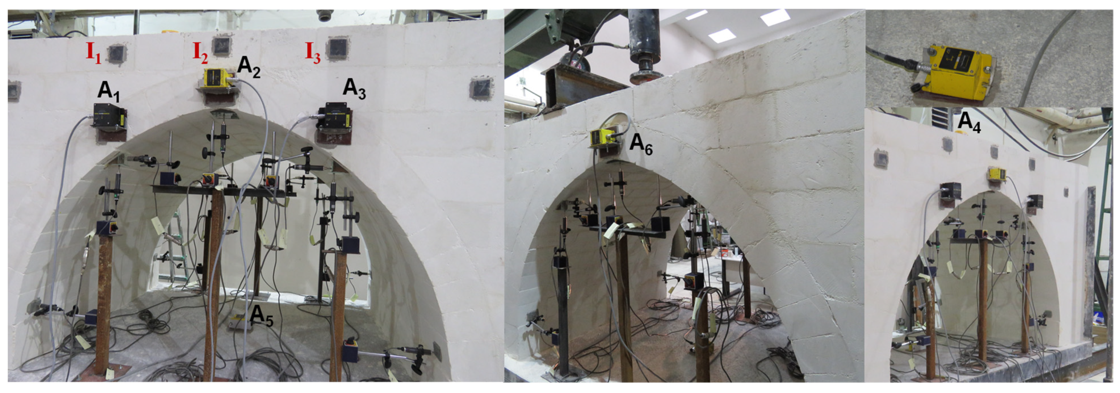
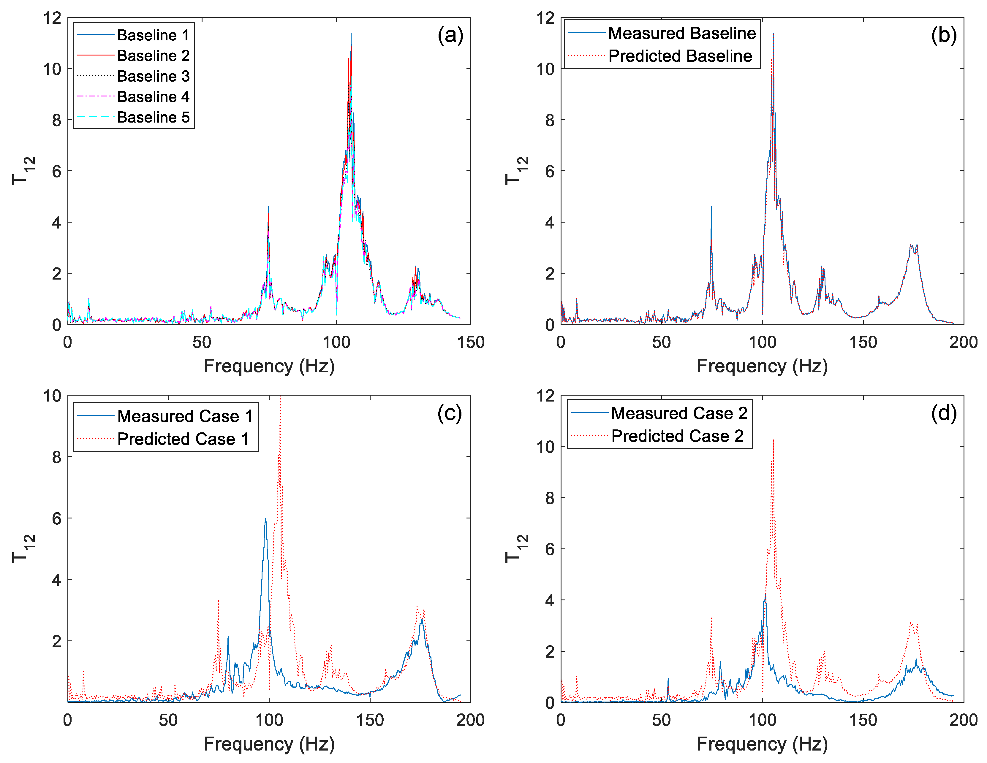
3.2. Experimental Study: Masonry Arch Bridge Model

The test specimen shown in Figure 8 consisted of an arch ring with a span of 1.73 m and a rise of 0.94 m. It had an overall width of 1.4 m, encompassing both the spandrel walls and the fill. A 10 cm thick reinforced concrete slab, with plan dimensions of 3.20 × 1.55 m, served as the foundation for the bridge model. The specimen was subjected to progressive damage by incremental increase in the vertically applied loading at the quarter length of the specimen. The load levels were set as 30 kN (Case 1) and 60 kN (Case 2) before the collapse load of 70 kN. Each loading case, except for the collapse case, included three repetitions of loading–unloading cycles, with impact tests conducted after the third cycle of unloading to monitor the structural response. Prior to pushing the structure to its collapse state, the accelerometers were disassembled to prevent damage to the instrumentation. Details of the static testing are available in [46].

A total of six accelerometers were mounted on the structure to collect acceleration measurements: four triaxial (A₂, A₄, A₅, A₆) and two unidirectional (A₁, A₃). The arrangement of the accelerometers and the impact locations are shown in Figure 9. The impact tests carried out at the baseline state were repeated five times to generate five independent datasets for training. The acceleration responses in the vertical direction (A₁, A₂, A₃, and A₆) due to impacts in the same direction at locations I₁, I₂, and I₃ were processed to generate the local TFs: T₁₂, T₂₃, T₄₂, and T₆₂ at the baseline state. After loading the specimen to the preset load levels and inflicting damage states shown in Figure 10, the same measurements were collected in the same manner to obtain the TFs for damage scenarios of Cases 1–2.

Using the baseline dataset, a conventional AE with a single hidden layer of 10 neurons was trained to reconstruct each transmissibility. Figure 11a,b displays the dataset for the baseline state and compares the measured with the AE prediction for T₁₂. The comparison between the measured and predicted values for the damage states of Case 1 and 2 is shown in Figure 11c,d.

The reconstruction errors from the baseline state were then used as DSF for training an OC-SVM to aid in the damage detection decision. The detection performance of these features is clearly displayed in Figure 12a, where the first two features of the damage states are compared to those of the baseline state. To locate the damaged region around the arch, localization index DI was formulated using only the sensors on the front face of the arch, specifically T₁₂ and T₂₃. With this arrangement, the spatial resolution for damage.

Localization was limited to two regions between three sensors: between sensors 1 and 2 (A₁–A₂) or sensors 2 and 3 (A₂–A₃), as shown previously in Figure 9. The localization results obtained with DI are displayed in Figure 12b. As shown in this figure, damage localized between sensors 2 and 3 progresses into the region between sensors 1 and 2 as the load level increases from 30 kN to 60 kN.

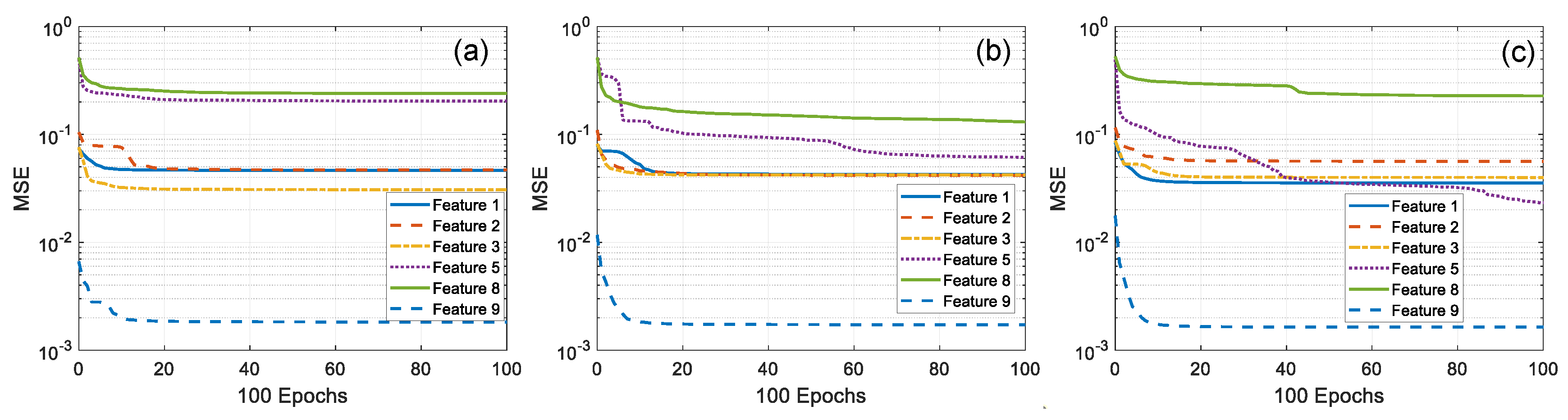
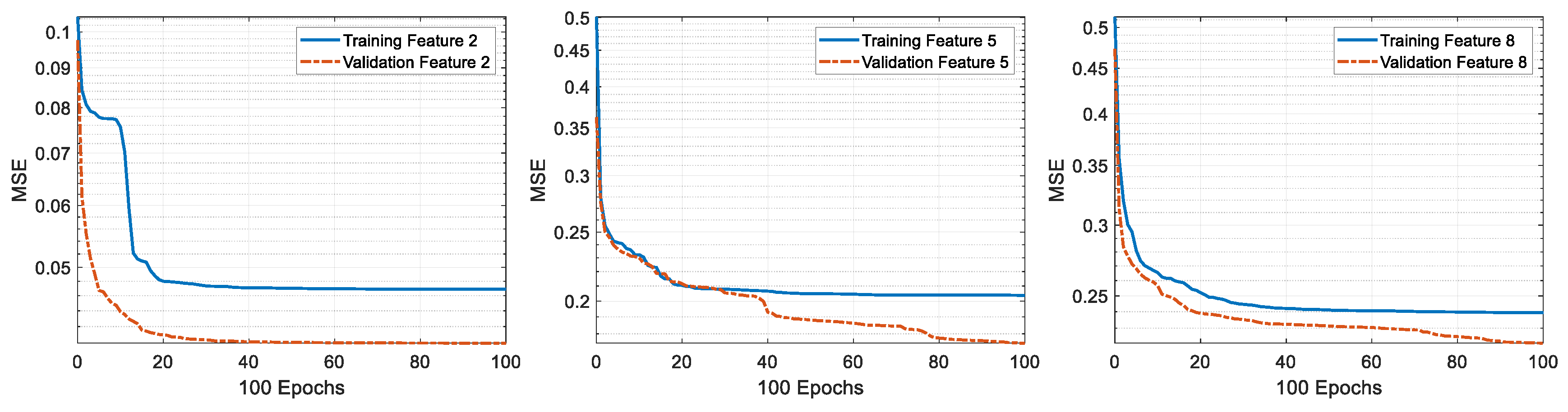
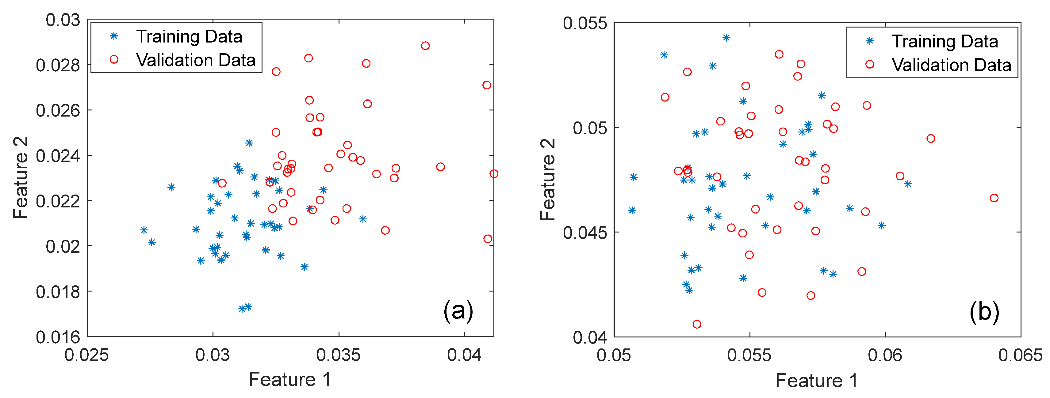
4. Discussion on Noise Effects, Model Selection, and Feature Sensitivity

To investigate the effect of noise, the noise intensity level in the numerical simulation study was increased up to 10%. A total of 40 sets of noise-contaminated training data and 220 sets of test data were generated, with 180 corresponding to damage scenarios and 40 representing the healthy state for validation. It should be noted that the damage scenarios considered in this study represent light damage cases, with a maximum stiffness loss of 20%, corresponding to frequency shifts of up to 2.8%. Given the relatively small severity of these damage cases, further increase in the noise level would not be meaningful, as detecting very light damage under excessively high noise conditions is not a realistic expectation in practical SHM applications.

The detection performance of the proposed methodology for all the damage cases, including the healthy state validation data at 10% noise level, is summarized in

Table 4. Confusion matrix for the numerical study (noise level = 10%): PCA versus AE with OC-SVM.

		PCA			AE
		Predicted			Predicted
		Healthy	Damaged	Total	Healthy	Damaged	Total
True	Healthy	70%	30%	40	75%	25%	40
	Damage Case 1	35%	65%	20	5%	95%	20
	Damage Case 2	20%	80%	20	5%	95%	20
	Damage Case 3	100%	0%	20	5%	95%	20
	Damage Case 4	65%	35%	20	5%	95%	20
	Damage Case 5	50%	50%	20	45%	55%	20
	Damage Case 6	75%	25%	20	5%	95%	20
	Damage Case 7	60%	40%	20	15%	85%	20
	Damage Case 8	10%	90%	20	5%	95%	20
	Damage Case 9	5%	95%	20	0%	100%	20

. The AE outperformed PCA even as the noise level increased. With the AE model, the critical Type II error—failing to issue an alert when damage is present—which was non-existent previously at lower noise levels, was calculated to be 10% at this noise level. Meanwhile, Type I error—false damage alarms—increased from 5% to 25%. As expected, lower noise levels yield more precise damage identification results. Hence, the proposed scheme is robust against moderate noise levels. Damage localization results, on the other hand, became unreliable for all damage cases except Damage Case 1 with increased noise level. This suggests that the pattern in the reconstruction error, which serves as a key indicator of damage location, is significantly affected by increased noise contamination for the light damage levels considered.

To assess the effectiveness of OC-SVM as a classifier, a comparison was made with isolation forest (iForest), an alternative anomaly detection algorithm. iForest was chosen for its ability to identify outliers via recursive partitioning, which is particularly well-suited for structural damage detection, as it isolates anomalies directly without requiring prior labeling of the data. This makes it a more robust choice compared to clustering-based methods, which typically require assumptions about cluster shapes.

Table 5. Detection performance of AE: iForest versus OC-SVM (SNR = 10%).

		iForest Predicted		OC-SVM Predicted
		Healthy	Damaged	Healthy	Damaged
True	Healthy	95%	5%	75%	25%
	Damage Case 1	5%	95%	5%	95%
	Damage Case 2	10%	90%	5%	95%
	Damage Case 3	30%	70%	5%	95%
	Damage Case 4	55%	45%	5%	95%
	Damage Case 5	75%	25%	45%	55%
	Damage Case 6	75%	25%	5%	95%
	Damage Case 7	75%	25%	15%	85%
	Damage Case 8	55%	45%	5%	95%
	Damage Case 9	0%	100%	0%	100%

presents the comparative results of OC-SVM and iForest in detecting structural damage. The OC-SVM method utilizes a hyperplane-based decision boundary to classify data, while iForest adopts a tree-based approach, isolating outliers.

In terms of error rates, iForest demonstrated an improvement in the Type I error (false positive rate), reducing it to 5%, compared to OC-SVM’s higher rate of 25%. However, this improvement in Type I error came at the expense of an increase in Type II errors (false negative rate), which rose from 10%, the average for nine damage cases in OC-SVM, to 42.2% for iForest. While iForest effectively reduces false positives, it may be more conservative in detecting all damage cases, potentially leading to missed detection of actual damage, which is critical from a safety perspective in SHM. OC-SVM, on the other hand, maintains a more balanced performance.

With a single hidden-layer AE architecture employed in this study, finding the optimum number of neurons proved to be critical, as the hidden layer directly serves as the latent space. The number of neurons determines the dimension of this space, affecting how well damage-sensitive features are captured. The results reported in Table 2 for the model with three neurons led to 5% Type I and 0% Type II errors. Increasing the number of neurons to 10 increased the false positives, impairing generalization and resulted in a Type I error of 30%. and a Type II error of 11%. Additionally, with increased neuron size, localization performance deteriorated and led to false identifications in half of the damage cases.

Furthermore, the potential of utilizing latent space features was explored as an alternative indicator sensitive to damage. Figure 13 presents a comparison of the first two latent space features extracted from the training and test data for the selected TFs under varying noise levels. Interestingly, the clustering behavior of the latent features was inconsistent across different TFs. For some TFs, a distinct clustering between damaged and undamaged cases was observed even at higher noise levels, while for others, clustering was more prominent at lower noise levels. Increasing the number of neurons or hidden layers does not necessarily lead to improved results. This suggests that the latent space features’ sensitivity to damage may vary depending on the TF, and noise may have a no linear interaction with these features, potentially affecting their robustness. Such inconsistencies require further investigation to better understand the underlying mechanisms that govern the relationship between noise, damage sensitive features, and damage detection performance.

5. Conclusions

With their ability to automatically identify patterns and detect anomalies without requiring an explicit physical model of the structure, machine learning tools are instrumental in exploiting the full potential of SHM. Unsupervised approaches, which do not require labeled training data from various damage scenarios, are particularly crucial for civil engineering systems where collecting diverse damage data is difficult, if not impossible. With training data that can adequately capture variations in operational and environmental conditions at the baseline state, these methods allow for distinguishing damage-induced changes in sensor readings from those caused by such variations.

Building on this machine-learning perspective, this paper presents a damage identification methodology implementing an AE trained on measured data from the baseline state of the structural system. As a highly suitable feature for output-only SHM applications, transmissibility calculated directly from the acceleration measurements is used as input to the AE to capture the healthy-system response and effectively characterize the structural system’s dynamic properties. The reconstruction errors generated by the trained model from the transmissibility input serve explicitly as the damage-sensitive feature in training the OC-SVM for damage classification. The trained AE processes input data from different structural states, producing reconstruction errors that are subsequently evaluated by the OC-SVM to determine whether there is damage. For the state detected as ‘damaged’, the proposed damage index is used to determine the location of the damage within the provided sensor resolution.

The numerical investigations demonstrated the advantages of incorporating nonlinear encoding into dimensionality reduction by the improved reconstruction accuracy and robustness of the AE compared to a classical method of PCA. More specifically, while PCA provides a closed-form solution for projecting data onto a lower-dimensional subspace, preserving maximum variance, the AE introduces nonlinear transformations and learns the components indirectly through optimization that may be instrumental in enhancing the data representation. Experimental data from a masonry arch bridge model validated the proposed approach to detect and locate damage in an unsupervised manner using only a small set of training data to track the health state of the system. Since the proposed methodology does not require a finite element model but operates in a fully data-driven fashion, the localization performance is clearly limited with the resolution of sensor locations.

The damage detection aspect of the proposed methodology is proven to be robust, even in the presence of noisy data. However, the accuracy of damage localization is highly dependent/more sensitive on precise sensor data. The reconstruction error, as a damage-sensitive feature, proves to be more consistent and reliable compared to the latent space features, which exhibit greater variability. Incorporating a one-class classification algorithm eliminates the need for a pre-determined threshold and offers flexibility and adaptability in detecting damage. More specifically, OC-SVM has been shown to handle varying data characteristics and noise levels effectively.

In conclusion, the proposed unsupervised methodology requires only measured acceleration response signals from the structure. The only limitation of the technique is that it requires impact testing across multiple locations to generate a comprehensive set of TFs. However, with a model-free approach that can be employed in an unsupervised manner, this is a manageable trade-off. Recent advances in impact testing methodologies and mobile sensing systems that can navigate throughout the structure may help mitigate this limitation.

For future work, incorporating physics-informed machine learning techniques could enhance the interpretability and reliability of the proposed methodology. By integrating domain knowledge into the learning process, physics-informed models can improve generalization, especially in cases with limited data. Additionally, while the current methodology does not utilize measurements during strong-motion phases, future work could explore integrating our approach with existing strategies that focus on capturing variations in damage sensitive features during high-intensity loading events. Since the frequency content of such vibration data is richer and contains more complex information, combining these insights with the transmissibility-based approach could contribute to a more comprehensive damage detection system capable of operating under a wider range of conditions.

References

1. Avci, O.; Abdeljaber, O.; Kiranyaz, S.; Hussein, M.; Gabbouj, M.; Inman, D.J. A Review of Vibration-Based Damage Detection in Civil Structures: From Traditional Methods to Machine Learning and Deep Learning Applications. Mech. Syst. Signal Process. 2021, 147, 107077. [Google Scholar]
2. Rafiei, M.H.; Adeli, H. A Novel Unsupervised Deep Learning Model for Global and Local Health Condition Assessment of Structures. Eng. Struct. 2018, 156, 598–607. [Google Scholar]
3. Entezami, A.; Shariatmadar, H.; Karamodin, A. Data-Driven Damage Diagnosis under Environmental and Operational Variability by Novel Statistical Pattern Recognition Methods. Struct. Health Monit. 2019, 18, 1416–1443. [Google Scholar]
4. Zhang, H.; Gül, M.; Kostić, B. Eliminating Temperature Effects in Damage Detection for Civil Infrastructure Using Time Series Analysis and Autoassociative Neural Networks. J. Aerosp. Eng. 2019, 32, 04019001. [Google Scholar]
5. Sarmadi, H.; Karamodin, A. A Novel Anomaly Detection Method Based on Adaptive Mahalanobis-Squared Distance and One-Class kNN Rule for Structural Health Monitoring under Environmental Effects. Mech. Syst. Signal Process. 2020, 140, 106495. [Google Scholar]
6. Wang, Z.; Cha, Y.J. Unsupervised Machine and Deep Learning Methods for Structural Damage Detection: A Comparative Study. Eng. Rep. 2022, 7, e12551. [Google Scholar]
7. Soofi, Y.J.; Bitaraf, M. Output-Only Entropy-Based Damage Detection Using Transmissibility Function. J. Civ. Struct. Health Monit. 2022, 12, 191–205. [Google Scholar]
8. Liu, L.; Zhang, X.; Lei, Y. Data-Driven Identification of Structural Damage under Unknown Seismic Excitations Using the Energy Integrals of Strain Signals Transformed from Transmissibility Functions. J. Sound Vib. 2023, 546, 117490. [Google Scholar]
9. Bank, D.; Koenigstein, N.; Giryes, R. Autoencoders. In Machine Learning for Data Science Handbook: Data Mining and Knowledge Discovery Handbook; Springer: Cham, Switzerland, 2023; pp. 353–374. [Google Scholar]
10. Berahmand, K.; Daneshfar, F.; Salehi, E.S.; Li, Y.; Xu, Y. AEs and Their Applications in Machine Learning: A Survey. Artif. Intell. Rev. 2024, 57, 28. [Google Scholar]
11. Pathirage, C.S.N.; Li, J.; Li, L.; Hao, H.; Liu, W.; Ni, P. Structural Damage Identification Based on AE Neural Networks and Deep Learning. Eng. Struct. 2018, 172, 13–28. [Google Scholar]
12. Anaissi, A.; Zandavi, S.M. Multi-Objective AE for Fault Detection and Diagnosis in Higher-Order Data. In Proceedings of the 2019 International Joint Conference on Neural Networks (IJCNN), Budapest, Hungary, 14–19 July 2019; pp. 1–8. [Google Scholar]
13. Lee, K.; Jeong, S.; Sim, S.H.; Shin, D.H. A Novelty Detection Approach for Tendons of Prestressed Concrete Bridges Based on a Convolutional AE and Acceleration Data. Sensors 2019, 19, 1633. [Google Scholar] [PubMed]
14. Ma, X.; Lin, Y.; Nie, Z.; Ma, H. Structural Damage Identification Based on Unsupervised Feature-Extraction via Variational AE. Measurement 2020, 160, 107811. [Google Scholar]
15. Yan, X.; Liu, Y.; Jia, M. Health Condition Identification for Rolling Bearing Using a Multi-Domain Indicator-Based Optimized Stacked Denoising AE. Struct. Health Monit. 2020, 19, 1602–1626. [Google Scholar]
16. Rastin, Z.; Ghodrati Amiri, G.; Darvishan, E. Unsupervised Structural Damage Detection Technique Based on a Deep Convolutional AE. Shock Vib. 2021, 2021, 6658575. [Google Scholar]
17. Wang, Z.; Cha, Y.J. Unsupervised Deep Learning Approach Using a Deep AE with a One-Class Support Vector Machine to Detect Damage. Struct. Health Monit. 2021, 20, 406–425. [Google Scholar]
18. Lee, K.; Jeong, S.; Sim, S.H.; Shin, D.H. Field Experiment on a PSC-I Bridge for Convolutional AE-Based Damage Detection. Struct. Health Monit. 2021, 20, 1627–1643. [Google Scholar]
19. Jiang, K.; Han, Q.; Du, X.; Ni, P. A Decentralized Unsupervised Structural Condition Diagnosis Approach Using Deep AEs. Comput.-Aided Civ. Infrastruct. Eng. 2021, 36, 711–732. [Google Scholar]
20. Silva, M.F.; Santos, A.; Santos, R.; Figueiredo, E.; Costa, J.C.W.A. Damage-sensitive feature extraction with stacked AEs for unsupervised damage detection. Struct. Control Health Monit. 2021, 28, e2714. [Google Scholar]
21. Shang, Z.; Sun, L.; Xia, Y.; Zhang, W. Vibration-based damage detection for bridges by deep convolutional denoising AE. Struct. Health Monit. 2021, 20, 1880–1903. [Google Scholar]
22. Zhang, Y.; Xie, X.; Li, H.; Zhou, B. An unsupervised tunnel damage identification method based on convolutional variational auto-encoder and wavelet packet analysis. Sensors 2022, 22, 2412. [Google Scholar] [CrossRef]
23. Spínola Neto, M.; Finotti, R.; Barbosa, F.; Cury, A. Structural Damage Identification Using AEs: A Comparative Study. Buildings 2024, 14, 2014. [Google Scholar]
24. Römgens, N.; Abbassi, A.; Jonscher, C.; Grießmann, T.; Rolfes, R. On using AEs with non-standardized time series data for damage localization. Eng. Struct. 2024, 303, 117570. [Google Scholar]
25. Li, Z.; Lin, W.; Zhang, Y. Real-time drive-by bridge damage detection using deep auto-encoder. Structures 2023, 47, 1167–1181. [Google Scholar]
26. Li, L.; Morgantini, M.; Betti, R. Structural damage assessment through a new generalized AE with features in the quefrency domain. Mech. Syst. Signal Process. 2023, 184, 109713. [Google Scholar] [CrossRef]
27. Lin, J.; Ma, H. Structural damage detection based on the correlation of variational AE neural networks using limited sensors. Sensors 2024, 24, 2616. [Google Scholar]
28. Li, S.; Cao, Y.; Gdoutos, E.E.; Tao, M.; Alkayem, N.F.; Avci, O.; Cao, M. Intelligent framework for unsupervised damage detection in bridges using deep convolutional AE with wavelet transmissibility pattern spectra. Mech. Syst. Signal Process. 2024, 220, 111653. [Google Scholar]
29. Resende, L.V.; Finotti, R.P.; Barbosa, F.S.; Cury, A.A. Structural damage detection with autoencoding neural networks. In Proceedings of the XLIII Ibero-Latin American Congress on Computational Methods in Engineering, Foz do Iguacu, Brazil, 21–25 November 2022; Volume 4, p. 4. [Google Scholar]
30. Nicoletti, V.; Quarchioni, S.; Amico, L.; Gara, F. Assessment of different optimal sensor placement methods for dynamic monitoring of civil structures and infrastructures. Struct. Infrastruct. Eng. 2024, 1–16. [Google Scholar] [CrossRef]
31. Mendler, A.; Döhler, M.; Ventura, C.E. Sensor placement with optimal damage detectability for statistical damage detection. Mech. Syst. Signal Process. 2022, 170, 108767. [Google Scholar]
32. Wang, Y.; Chen, Y.; Yao, Y.; Ou, J. Advancements in Optimal Sensor Placement for Enhanced Structural Health Monitoring: Current Insights and Future Prospects. Buildings 2023, 13, 3129. [Google Scholar] [CrossRef]
33. Sun, Z.; Mahmoodian, M.; Sidiq, A.; Jayasinghe, S.; Shahrivar, F.; Setunge, S. Optimal Sensor Placement for Structural Health Monitoring: A Comprehensive Review. J. Sens. Actuator Netw. 2025, 14, 22. [Google Scholar] [CrossRef]
34. Chesné, S.; Deraemaeker, A. Damage localization using transmissibility functions: A critical review. Mech. Syst. Signal Process. 2013, 38, 569–588. [Google Scholar] [CrossRef]
35. Li, J.; Hao, H.; Lo, J.V. Structural damage identification with power spectral density transmissibility: Numerical and experimental studies. Smart Struct. Syst. 2015, 15, 15–40. [Google Scholar] [CrossRef]
36. Zhu, D.; Yi, X.; Wang, Y. A local excitation and measurement approach for decentralized damage detection using transmissibility functions. Struct. Control Health Monit. 2016, 23, 487–502. [Google Scholar] [CrossRef]
37. Zhou, Y.L.; Maia, N.M.; Abdel Wahab, M. Damage detection using transmissibility compressed by principal component analysis enhanced with distance measure. J. Vib. Control 2018, 24, 2001–2019. [Google Scholar] [CrossRef]
38. Yan, W.J.; Zhao, M.Y.; Sun, Q.; Ren, W.X. Transmissibility-based system identification for structural health monitoring: Fundamentals, approaches, and applications. Mech. Syst. Signal Process. 2019, 117, 453–482. [Google Scholar] [CrossRef]
39. Liu, T.; Xu, H.; Ragulskis, M.; Cao, M.; Ostachowicz, W. A data-driven damage identification framework based on transmissibility function datasets and one-dimensional convolutional neural networks: Verification on a structural health monitoring benchmark structure. Sensors 2020, 20, 1059. [Google Scholar] [CrossRef]
40. Lei, Y.; Zhang, Y.; Mi, J.; Liu, W.; Liu, L. Detecting structural damage under unknown seismic excitation by deep convolutional neural network with wavelet-based transmissibility data. Struct. Health Monit. 2021, 20, 1583–1596. [Google Scholar] [CrossRef]
41. Entezami, A.; Sarmadi, H.; Salar, M.; De Michele, C.; Arslan, A.N. A novel data-driven method for structural health monitoring under ambient vibration and high-dimensional features by robust multidimensional scaling. Struct. Health Monit. 2021, 20, 2758–2777. [Google Scholar] [CrossRef]
42. Ozdagli, A.I.; Koutsoukos, X. Machine learning-based novelty detection using modal analysis. Comput. Aided Civ. Inf. Eng. 2019, 34, 1119–1140. [Google Scholar] [CrossRef]
43. Maia, N.M.M.; Urgueira, A.P.V.; Almeida, R.A.B. An overview of the transmissibility concept and its application to structural damage detection. In Topics in Modal Analysis I, Volume 5, Conference Proceedings of the Society for Experimental Mechanics Series; Allemang, R., De Clerck, J., Niezrecki, C., Blough, J., Eds.; Springer: New York, NY, USA, 2012; pp. 317–330. [Google Scholar] [CrossRef]
44. Hejazi, M.; Singh, Y.P. One-class support vector machines approach to anomaly detection. Appl. Artif. Intell. 2013, 27, 351–366. [Google Scholar] [CrossRef]
45. Schölkopf, B.; Williamson, R.C.; Smola, A.; Shawe-Taylor, J.; Platt, J. Support vector method for novelty detection. In Neural Information Processing Systems; MIT Press: Cambridge, MA, USA, 2000; pp. 582–588. [Google Scholar]
46. Mentese, V.G.; Gunes, O.; Celik, O.C.; Gunes, B.; Avsin, A.; Yaz, M. Experimental collapse investigation and nonlinear modeling of a single-span stone masonry arch bridge. Eng. Fail. Anal. 2023, 152, 107520. [Google Scholar] [CrossRef]
Figure 1. Damage detection methodology.
Applsci 15 04098 g001
Figure 2. Architecture of a traditional undercomplete AE.
Applsci 15 04098 g002
Figure 3. Simulated system with sensor locations and system properties.
Applsci 15 04098 g003
Figure 4. MSE for the training data of the AE with varying numbers of neurons (n): (a) n = 1, (b) n = 3, (c) n = 5.
Applsci 15 04098 g004
Figure 5. MSE comparison for training versus validation data for n = 3 neurons.
Applsci 15 04098 g005
Figure 6. Distribution of the first two DSFs for the training and validation data: (a) PCA; (b) AE.
Applsci 15 04098 g006
Figure 7. Damage localization results using the AE: (ai) D. Cases 1–9.
Applsci 15 04098 g007
Figure 8. Test specimen: (a) static loading; (b) impact testing.
Applsci 15 04098 g008
Figure 9. Accelerometer (A1–A6) and impact locations (I1–I3).
Applsci 15 04098 g009
Figure 10. Observed damage after loading up to: (a) 30 kN; (b) 60 kN; (c) collapse at 70 kN.
Applsci 15 04098 g010
Figure 11. T12 comparisons (a) measured data at the baseline state (bd) measured versus AE predicted for the baseline and the damage cases.
Applsci 15 04098 g011
Figure 12. (a) Damage detection features; (b) damage localization for Cases 1 and 2.
Applsci 15 04098 g012
Figure 13. Latent space features for transmissibility functions T34 and T56: (a,c) Low noise level (2–5%); (b,d) high noise level (10%).
Applsci 15 04098 g013