Article

Algorithm for Extraction of Reflection Waves in Single-Well Imaging Based on MC-ConvTasNet

Department of Mechanics, Harbin Institute of Technology, Harbin 150001, China
*
Author to whom correspondence should be addressed.
Appl. Sci. 2025, 15(8), 4189; https://doi.org/10.3390/app15084189
Submission received: 10 March 2025 / Revised: 7 April 2025 / Accepted: 8 April 2025 / Published: 10 April 2025
(This article belongs to the Special Issue Seismic Analysis and Design of Ocean and Underground Structures)

Abstract

:
Single-well imaging makes use of reflected waves to image geological structures outside a borehole, with a detection distance expected to reach tens of meters. However, in the received full wave signal, reflected waves have much smaller amplitudes than borehole-guided waves, which travel directly through the borehole. To obtain clear reflected waves, we use a deep neural network, the multi-channel convolutional time-domain audio separation network (MC-ConvTasNet), to extract reflected waves. In the signal channels of the common-source gather, there exists a notable arrival time difference between direct waves and reflected waves. Leveraging this characteristic, we train MC-ConvTasNet on the common-source gathers, ultimately achieving satisfactory results in wave separation. For the hard-to-hard single-interface, soft-to-hard single-interface and double-interface models, the reflected waves extracted by MC-ConvTasNet are closer to the theoretical reflected waves in both phase and shape (the average scale-invariant signal-to-distortion ratio exceeds 32 dB) than those extracted by parameter estimation, a median filter and an F-K filter. Meanwhile, MC-ConvTasNet naturally fits in the scenarios of various inclined interfaces and interfaces parallel to the borehole axis. As an application, our method is employed on field logging data and its ability to separate waves is verified.

1. Introduction

In the process of acoustic logging, most of the energy excited by an acoustic source propagates along the borehole wall, known as the direct wave. A small amount of energy radiates to the formation outside the borehole and is reflected back to the borehole by the geologic interface in the formation, forming reflected waves [1]. Conventional acoustic logging usually uses the direct wave, which has a relatively close detection distance. Sonic reflection imaging uses the reflected wave to detect the geological structures outside the borehole, and the depth of detection is usually several meters to tens of meters [2], which greatly extends the radial detection distance of acoustic logging. In recent years, there has been a lot of research on single-well imaging [3,4,5]. However, in the full wave signal received by the acoustic logging tool, the reflected wave has a much smaller amplitude than the direct wave. The earlier part of the reflected wave is often covered by the tail of the direct wave. Thus, it is difficult to separate them. One of the core difficulties of single-well imaging is obtaining a clear reflected wave signal from the received full waveform.
Many methods have been proposed for extracting reflected arrivals from logging data. For common-source gather (CSG) data, a 2-D adaptive prediction error filter [6] and wave field separation filter combining parametric decomposition and waveform inversion [7] can separate reflected signals. Tang et al. [8] suggest a parameter estimation method for CSG and common-receiver gather (CRG) data to separate downgoing and upgoing waves, respectively. For common-offset gather (COG) data, an F-K filter [9], high-resolution Radon transform [10], Karhunen–Loève transform [11], shear wave transform [12] and unsupervised machine learning [13] are proposed for wave separation. Median filters can be applied to COG [1], CSG and CRG [14] data to extract the reflected waves. However, the extraction methods mentioned above have intrinsic drawbacks. The parameter estimation and the wave field separation filter combining parametric decomposition and waveform inversion can only suppress part of the direct wave. The computational efficiency of the high-resolution Radon transform is low. The amplitude of reflected waves extracted by a median filter is jagged. Methods applied to COG data are not suitable for the cases in which the interface is parallel to the borehole axis. A clear and complete reflected wave is essential for high-quality imaging results. Therefore, it is necessary to propose a convenient and reliable method for extracting reflected waves.
The separation of the reflected wave and direct wave in the recorded full wavetrains in the borehole has similarities to the separation of the target waveform and the interference waveform (or background noise) in speech separation [15]. In the borehole problem, the signal is excited by a single acoustic source. The signal that reaches the receiver through the well is a direct wave. The signal returned through the reflection interface is called the reflected wave. In speech separation, the reflected wave that can be distinguished from the direct wave is called echo. The reflected wave that overlaps the direct waveform is called reverberation. The borehole problem is similar to the indoor mono-source scenario problem in speech separation. There are many neural networks with good performance, fast filtering speed and high accuracy in the field of speech separation which can be used as a reference for solving the problem of reflected wave extraction.
Many speech separation methods are performed in the time–frequency domain of the signal [16,17,18]. In general, the signal is converted into a spectrogram using short-time Fourier transform, and then the neural network performs speech separation in the time–frequency domain [19]. Since the short-time Fourier transform usually only deals with the amplitude spectrum, the phase information may be inaccurate in the reconstruction, resulting in degraded speech quality [20]. The time-domain method usually adopts the end-to-end deep learning model, which can directly learn the separated features from the original waveform, avoiding the intermediate step of time–frequency domain conversion, and the reconstructed speech quality is usually higher. Wave-U-Net [21], which is built upon the architecture of U-Net, integrates multiscale analysis and temporal domain processing for speech separation. Compared with the time–frequency domain method, Wave-U-Net has a simple structure and outstanding effect. Thereafter, Luo and Mesgarani [22] proposed a convolutional time-domain audio separation network (Conv-TasNet) for speech separation. In Conv-TasNet, a linear encoder maps the mixed waveform to an encoded representation. Stacked dilated 1-D convolutional blocks then act as a separation module to separate encoded representations from different acoustic sources. The encoded representation containing a single sound source is then transformed into the desired source waveform using a linear decoder. Due to its superior performance, it is used in logging [23].
Because the quality of speech separation is greatly improved by multiple channels [15], this paper realizes the reflection wave extraction by analyzing the waveform signal of a multi-channel array. In the COG domain, both the direct wave and the reflected wave from parallel interfaces have a zero inter-channel arrival time difference, which is detrimental to separation by neural networks. However, single-well imaging is also used for reflectors approximately parallel to the wellbore axis. Due to the differences in propagation distance and velocity between the direct wave and the reflected wave, the wavefront arrival time and the arrival time difference between channels in the CSG are always different. Therefore, we choose to extract the reflected wave in the CSG domain. Conv-TasNet was originally proposed for single-channel separation tasks. Inspired by the inter-channel phase difference formula, Gu et al. [24] designed a new two-dimensional convolution kernel to calculate inter-channel convolution difference (ICD), supplementing Conv-TasNet with spatial clues and optimizing its parameters in a purely data-driven manner. That neural network hereafter is called MC-ConvTasNet. It works well for suppressing direct waves in this study.
To address the scarcity of labeled reflection waves in field logging data, we propose to generate a dataset based on analytic algorithms. Wave separation for dipole shear wave imaging can be regarded as a supervised learning problem, with the learning target being direct and reflected waves in the time domain. When using supervised learning to train neural networks, the training dataset must include the output target (also known as the label) for each corresponding input sample [25]. The reflectors in dipole shear wave imaging are typically located several meters to tens of meters away from the borehole, which presents a challenge for directly validating the correspondence between the imaging results and the actual geological structures. This makes it difficult to accurately infer pure reflected waves based on precise geological structure information. It is difficult to meet the training requirements of neural networks only by constructing a training dataset based on field logging data. In order to obtain an efficient reflected wave extraction system, it is necessary to simulate a large number of data. A fast forward algorithm is needed to simulate actual logging and output synthesized full waveforms. Kurkjian and Chang [26] derived an analytical expression for the displacement inside the borehole excited by the direct wave. The direct wave can be quickly synthesized by using the real axis integration method [27]. Xu and Hu [28] propose a fast forward algorithm for single-well imaging to calculate the borehole displacement excited by reflected waves. The synthesis of the dataset in this study benefits from the methods of the two aforementioned papers.
This article aims to utilize MC-ConvTasNet for the clear extraction of reflected waves. By synthesizing a large number of theoretical waveforms through analytical algorithms to train MC-ConvTasNet, it addresses the challenge of insufficient field logging data for forming a training dataset. The automatic separation of reflected waves is achieved, with the entire process requiring no additional manual intervention in the neural network and no prior acquisition of wellbore velocity information. In the field logging data, MC-ConvTasNet demonstrates impressive generalization ability, outperforming parameter estimation, a median filter and an F-K filter in suppressing direct waves. When the acoustic logging tool is continuously lifted, MC-ConvTasNet is capable of extracting reflected waves in real time, even when the interfaces are parallel to the wellbore axis.
The rest of the paper is organized as follows: Section 2 introduces the architecture of MC-ConvTasNet, the synthesis of the datasets, the loss function and training details. In Section 3, theoretical waveforms are synthesized for a hard-to-hard single-interface model, a soft-to-hard single-interface model and a double-interface model. The results of MC-ConvTasNet are compared to those of parameter estimation, a median filter and an F-K filter. Next, the wave separation capability of MC-ConvTasNet is verified using synthetic data with noise and field logging data. Finally, we compare the wave separation performance of MC-ConvTasNet and Wave-U-Net. In Section 4, we delve into the requirement for MC-ConvTasNet and its potential for widespread application.

2. Theory and Method
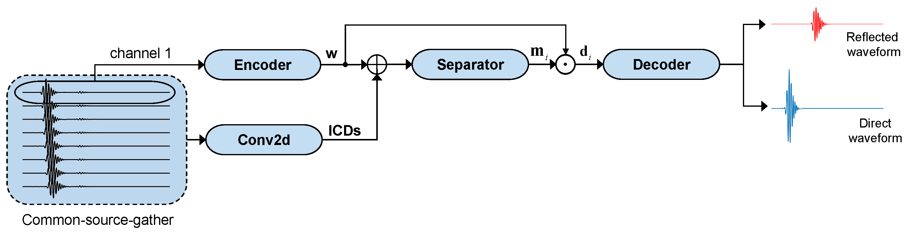
2.1. Network Model

Figure 1 shows a fluid-filled borehole surrounded by an elastic isotropic homogeneous formation. There is a geologic interface more than ten meters away from the borehole. The geologic interface hereafter is called a reflector. An array of receivers on the axis of the borehole receives both direct and reflected waves simultaneously.
The direct waves excited by a dipole source contain a flexural wave and a longitudinal wave. Because the longitudinal wave amplitude is very weak, it is ignored in the wave separation below. The reflected waves are SH-SH, SV-SV, P-P, P-SV and SV-P waves. The received displacement signal is
u = u 1 + u 2 ,
where u is the total displacement signal, and u 1 and u 2 are borehole displacements stimulated by the direct wave and reflected wave, respectively. The target of wave separation is to separate u 1 and u 2 in the received waveform. Traditional wave separation methods cannot effectively extract reflected waves. To improve the performance and efficiency of wave separation algorithms, we use MC-ConvTasNet for wave separation. The input data of MC-ConvTasNet are CSG-containing data from the channel currently being processed. The labels are the direct and reflected waves in the channel currently being processed. The propagation distance and velocity of the direct wave and the reflected wave are different, resulting in different arrival time differences between channels in the CSG. Therefore, a two-dimensional convolution (Conv2d) module is added to the MC-ConvTasNet to extract acoustic features between channels to help solve the problem of wave separation.
MC-ConvTasNet is composed of four parts, an encoder, Conv2d, a separator and a decoder, as shown in Figure 2. Firstly, the encoder module is used to transform the waveform of the channel currently being processed into its encoded representation. Secondly, the Conv2d module is used to extract the inter-channel convolution difference representation in the CSG, from which spatial clues can be obtained to help to distinguish direct and reflected waves. Then, the separator estimates the multiplication function (or mask) of the direct wave and reflected wave by using the encoded representation and the inter-channel convolution difference representation. Finally, the decoder module reconstructs the encoded representation of the direct or reflected wave back into the time-domain waveform of the direct or reflected wave in the channel currently being processed. The structure of MC-ConvTasNet is described in detail in the next section.

2.2. Network Architecture
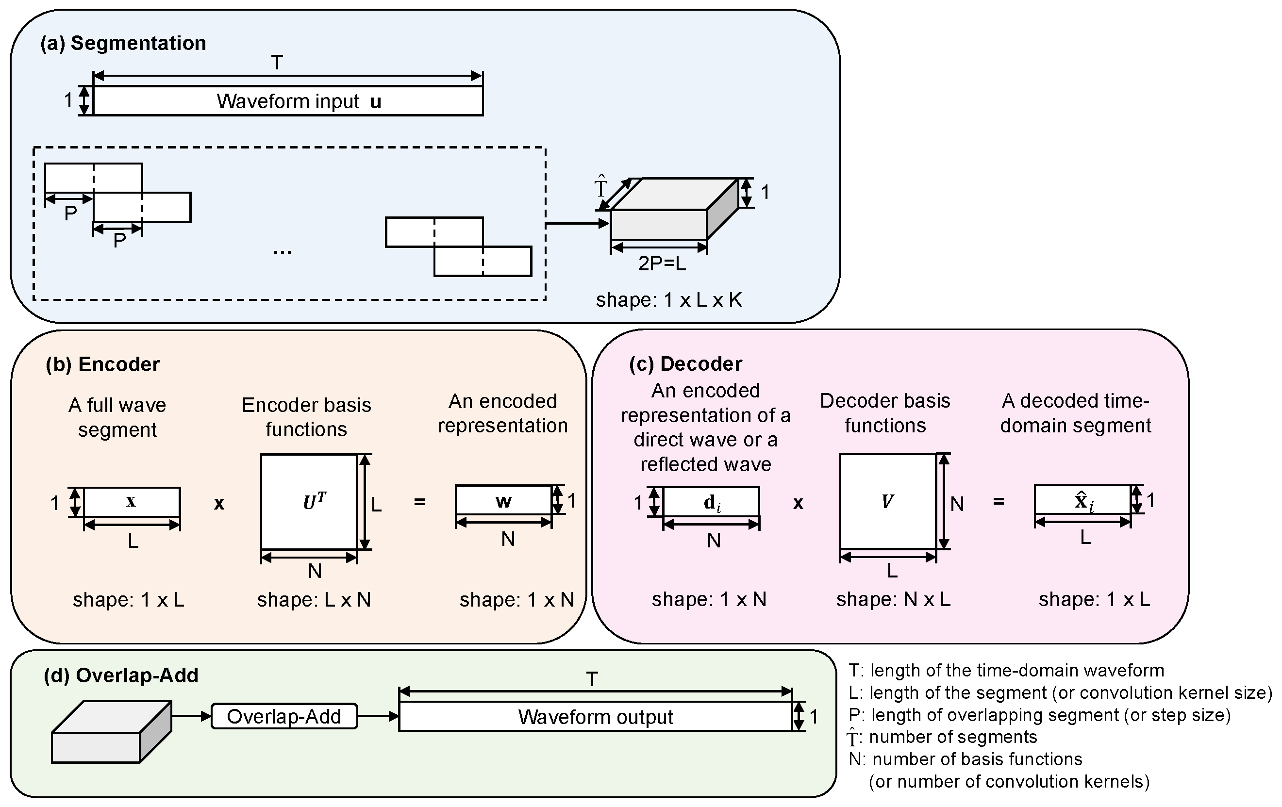
2.2.1. Encoder

The full waveform u R 1 × T of the encoder can be divided into overlapping segments of length L, represented by s k R 1 × L , where k = 1 , , T ^ represents the segment index, T ^ represents the total number of segments to be split and the overlap rate between fragments is 50% (see Figure 3a). The encoder converts s k to a one-dimensional vector of length N, w R 1 × N . This process can be represented by matrix multiplication (see Figure 3b), where x stands for s k ,
w = xU ,
where U R N × L is a matrix containing N vectors (encoder basis functions), with each vector having a length of L. In MC-ConvTasNet, the encoder is implemented by a 1-D convolution layer. One-dimensional convolution is different from convolution in mathematics. According to the convention of deep neural networks, performing segmentation and mapping on 1-D input data (Figure 3) is called 1-D convolution. The convolution kernel of 1-D convolution is learned during the training process. The convolution kernel size is 16, the step size is 8 and the number of convolution kernels is 512.

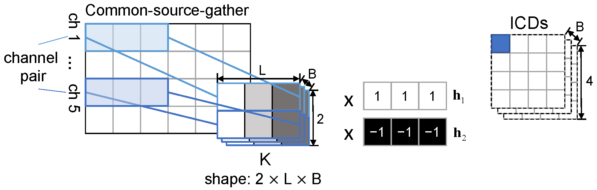
2.2.2. Conv2d (Spatial Feature Extraction)

In the CSG domain, the arrival time differences of the flexural wave and reflected wave between channels are different, which can be used to distinguish the flexural and reflected waves. The difference in the arrival time of the flexural wave between channels n 1 and n 2 is
Δ t f = d / v s ,
where d is the distance between receivers n 1 and n 2 , and v s is the velocity of the flexural wave. The differences in the arrival time of reflected waves between channels n 1 and n 2 are
Δ t P P = L 1 L 2 / α ,
Δ t S S = L 1 L 2 / β ,
Δ t P S = L ¯ S 1 L ¯ S 2 / β ,
Δ t S P = L ¯ P 1 L ¯ P 2 / α ,
where Δ t S S is the difference in arrival time of SH-SH and SV-SV waves; Δ t P P , Δ t P S and Δ t S P are the differences in arrival time of P-P, P-SV and SV-P waves, respectively; and α and β are the P-wave and S-wave velocities of the formation, respectively. For P-P, SH-SH and SV-SV waves, the reflection wave is of the same type as the incident wave. They share the same propagation distance for a given transmitter and receiver pair. L 1 and L 2 are the propagation distances from the acoustic source to the receivers n 1 and n 2 , respectively. The propagation distance is different for the converted SV wave from an incident P wave. L ¯ S 1 and L ¯ S 2 are the distances of the P-SV wave between the virtual force source and the receivers n 1 and n 2 , respectively. L ¯ P 1 and L ¯ P 2 are the distances of the SV-P wave between the virtual force source and the receivers n 1 and n 2 , respectively. Distances L 1 , L 2 , L ¯ S 1 , L ¯ S 2 , L ¯ P 1 and L ¯ P 2 were first derived by Xu and Hu [28] and are given in Appendix A. Since their calculation formulas are not required in the MC-ConvTasNet, they are not introduced in detail. Due to the differences in propagation distance and velocity, the arrival time differences of the direct wave and the reflected waves between channels are different, which helps to distinguish the direct wave and the reflected waves. The arrival time differences between channels in the time domain are related to the phase differences between channels in the frequency domain. The calculation formula for the inter-channel phase difference (ICD) is as follows:
Δ p n = Y n 1 Y n 2 ,
where Δ p n represents the inter-channel phase difference between the n-th pair of signal channels; Y n 1 and Y n 2 represent the complex spectrograms of the receiver n 1 and n 2 , respectively, obtained through the short-time Fourier transform; and ∠ represents the phase of the complex number, expressed in radians.
Inspired by the inter-channel phase difference formula, Gu et al. [24] designed a special 2-D convolution kernel to extract the ICD. The parameters of this Conv2d module learn in a data-driven manner, as shown in Figure 4. Like the waveform of the channel currently being processed, the c-th signal channel in the n-th pair of signal channels of the CSG can also be represented as overlapping segments of length L, expressed as y n c R 1 × L , where c = 1 , 2 represents the channel index in the channel pair, and n represents the channel pair index. For eight receivers, n = 1 , 2 , 3 , 4 . The filters of the spatial feature extraction module are K = { k ( b ) } R 2 × L × B , where B represents the number of filters and k ( b ) = k ( b ) k ( b ) 2 × L , k ( b ) R 1 × L is a filter that is shared across all signal channels to ensure the same mapping. The b-th ICD between the n-th pair of signal channels in the CSG can be expressed by the following formula [24]:
D n ( b ) = c = 1 2 h c · y n c k ( b ) ,
where D n ( b ) is one of the elements in the n-th row of the b-th ICD matrix; h c R 1 × L , c = 1 , 2 is a window function designed to smooth out the ICD and prevent potential spectrum leakage; and ⊙ represents the Hadamard product.
During training, h 1 is fixed as a matrix filled with ones, while h 2 is initialized to −1 and optimized with the other parameters. The ICD in the study of Gu et al. [24] was originally proposed for a circular microphone array. The farther apart the two channels in a channel pair are, the greater the phase difference. To extract phase difference information from eight receivers in a linear receiver array, we select four channel pairs, namely (1, 5), (2, 6), (3, 7) and (4, 8). In MC-ConvTasNet, the spatial information between the four pairs of channels is extracted by a 2-D convolution layer. The number of convolution kernels is 33, the convolution kernel size is (16, 2), the step size is (8, 1) and the expansion is (1, 4).

2.2.3. Separation

The separation module estimates the masks of the direct and reflected waves for each segment. Then, the encoded representation w of the full wave segment is multiplied by the mask m i R 1 × N , i = 1 , 2 to obtain separate encoded representations d i R 1 × N , i = 1 , 2 of the direct and reflected waves.
d i = w m i ,
where m i 0 , 1 , m 1 + m 2 = 1 . In the mask of reflected wave, the larger the proportion of energy expressed by the reflected wave after encoding, the closer the mask is to 1. The mask of the direct wave is constructed in a similar way. The separation module is consistent with Figure 1B in [22]. It mainly contains three fully convolutional separation modules. Each full convolution separation module consists of eight stacked 1-D dilated convolution blocks.

2.2.4. Decoder

The decoder reconstructs the waveform from the encoded representation of the direct wave or the reflected wave. The decoder can be reformulated as another matrix multiplication,
x ^ i = d i V ,
where x ^ i R 1 × L , i = 1 , 2 is the reconstructed segment of the direct wave and the reflected wave; and the rows of matrix V R N × L are the decoder basis functions, where each basis function has length L. The overlapping reconstructed segments are added together to produce the final waveform v ^ i R 1 × T , i = 1 , 2 (see Figure 3c) [29]. In MC-ConvTasNet, the decoder is implemented by a 1-D transposed convolution layer. The number of convolution kernels is 512, the convolution kernel size is 16 and the step size is 8.

2.3. Dataset

Field logging experiments cannot provide data for training because the interface outside the borehole is always unknown. We need to simulate theoretical waveforms as a dataset. In single-well imaging, 3-D finite-difference simulation is often used for forward simulation. However, it takes several hours to simulate the wave field for single-well imaging [30]. It is difficult to use for synthesizing a large number of waveforms in a dataset. Xu and Hu [28] propose an analytical three-step algorithm for quickly calculating theoretical reflection waves. Firstly, the far-field expression of radiated waves is obtained through the steepest-descent integration method [31]. Secondly, the reflected wave is equivalent to the radiation wave of a virtual source. The location and intensity of the virtual source are determined. Thirdly, an analytical expression for the borehole displacement response is obtained through the reciprocity relationship between point sources in a fluid–solid configuration [32]. Therefore, the theoretical full waveform can be synthesized by calculating the direct wave through the real axis integration method [27] and the reflected wave through the fast forward algorithm of single-well imaging [28,33]. Detailed calculation formulas for direct and reflected waves are shown in Appendix A. When calculating the dataset, we only consider faults. Although cavities are also a common geological feature in single-well imaging, in certain situations, they can be simplified and considered as faults.
In the forward calculation model of dipole S-wave imaging, the borehole radius is 0.1 m. The vibration of the acoustic source over time is cosine enveloped, with a center frequency of 3 kHz and a half-bandwidth of 2 kHz. The distance between the acoustic source and the first receiver is 112 inches. There are a total of eight receivers, with a spacing of 6 inches between them. The recording length in time of the full wave is 14.4 ms, with a time sampling interval of 10 μs.
The definitions of the distance, dip angle and azimuth angle for the reflector are illustrated in Figure 5. By changing the distance, dip angle and azimuth angle (as shown in Table 1), a total of 1092 spatial positions (=13 distances × 14 dip angles × 3 azimuth angles) of the reflectors are obtained. We generate 245,700 waveforms (=1092 spatial locations × 225 formation combinations × 8 receivers) as the dataset. The formations on both sides of the reflector are shown in Table 2. In the process of selecting formation parameters, we first determine the S-wave velocity. On the basis of Castagna’s mudrock line formula [34] ( α = 1.360 + 1.16 β ) and Li’s empirical formula [35] ( α = 0.0874 β 2 + 0.994 β + 1.250 ) for P-wave and S-wave velocities, we determine the corresponding P-wave velocity by incorporating computer-generated random values. The density is not completely independent and is related to the P-wave and S-wave velocities. Ma et al. [36] propose an empirical formula that fits all data without distinguishing rock types, revealing the relationship between density, P-wave velocity and S-wave velocity. The formula is expressed as ρ = 1.6289 α 0.2254 β 0.0924 , where ρ is the formation density. Based on this empirical formula, we generate the density values in the dataset by adding some computer-generated random values. Sedimentary rocks (such as shale, sandstone, limestone, mudstone and dolomite) are the most common geological conditions encountered in oil exploration. The ranges of P-wave velocity, S-wave velocity and density provided in Table 2 encompass these several common types of rocks. Although the formation medium parameters of the dataset are only a subset of the complex geological conditions, the trained neural network shows good generalization ability and can be applied to a variety of geological conditions. The range of the Poisson’s ratio of the formation in Table 2 is 0.095–0.462.
An inherent flaw of single-well imaging is that reflectors vertical to the borehole cannot be imaged. Hence, the dip angles in Table 1 do not include vertical or near-vertical situations. The azimuth angles of the dataset vary from 0° to 90°, which covers most types of reflected waves. Introducing more azimuthal angle variations does not significantly enhance the diversity of the data. The detection distance of single-well imaging is several meters to tens of meters [2]. While our analytical algorithms can theoretically analyze longer ranges, we set 13 m as the maximum distance in our dataset since reflected waves become more readily extractable as the reflector’s distance from the well increases. Of the dataset, 90% is selected as the training set, while the remaining 10% is used as the validation set. The test set consists of 34,944 waveforms (=1092 spatial locations × 4 formation combinations × 8 receivers). The four formation combinations contain soft and hard formations and do not appear in the training and validation sets.

2.4. Loss Function and Training Details

The loss function is determined based on the scale-invariant signal-to-distortion ratio. It achieves good general performance across a range of popular speech enhancement evaluation measures [37]. The scale-invariant signal-to-distortion ratio is defined as [38]
R std = 10 log 10 v target 2 2 e noisc 2 2 ,
where v target = v ^ · v v / v 2 2 , e noisc = v ^ v target , v is the ground-truth direct wave (or reflected wave) and v ^ is the estimated direct wave or reflected wave in the time domain. Zero mean normalization is applied to v and v ^ to ensure scale invariance. R std is defined in decibels (dB). The larger the R std , the closer v and v ^ . In order to ensure that the model parameters are optimal when the loss function is at its minimum in the optimization process, we define the loss function as R std . The optimization goal is to minimize the loss function, which is equivalent to maximizing the similarity between v and v ^ .
Batch normalization is used to speed up the separation process. During the training process, Adam [39] is used to optimize the parameters of the network such as the encoder basis functions, filters and decoder basis functions. The number of epochs is set to 60. The batch size is 512. The initial learning rate is 0.001. If the loss function on the validation set does not decrease for three consecutive epochs, the learning rate is halved. The remaining parameters of the network are consistent with the original Conv-TasNet paper [22]. The permutation problem of the direct wave and the reflected wave is solved by using utterance-level permutation-invariant training [18]. After training for 30 epochs, the reflected waves predicted by MC-ConvTasNet are closest to the theoretical reflected waves in the test set, with an average R std of 19.5.

3. Results

In this section, we compare the wave separation performance of MC-ConvTasNet, parameter estimation, a median filter and an F-K filter in three models. These three models are a hard-to-hard single-interface model, a soft-to-hard single interface model and a double-interface model (see Figure 6). We also verify the effectiveness of MC-ConvTasNet on the synthetic data with noise and the field logging data. To highlight the generalization capability of MC-ConvTasNet, we conduct a comparative analysis of its separation performance versus that of Wave-U-Net on field logging data. Data are analyzed using Python v3.7.
The formation parameters in the reflector models are shown in Table 3, and the formation combinations in this section do not appear in the training and validation sets. When the formation on the left side of interface 1 is formation 1 (hard formation), the forward calculation model is called a hard-to-hard single-interface model. When the formation on the left side of interface 1 is formation 2 (soft formation), the forward calculation model is called a soft-to-hard single-interface model. Interface 1 has an inclination of 10° with respect to the borehole axis and an azimuth of 0° with respect to the x-axis. The root mean square error and scale-invariant signal-to-distortion ratio are used as evaluation indexes. The root mean square error between the theoretical reflection wave v = q 1 , q 2 , , q T and the extracted reflection wave v ^ 1 = q ^ 1 , q ^ 2 , , q ^ T is defined as R rmse = 1 T i = 1 T ( q i q ^ i ) 2 , where T represents the length of the time-domain waveform. The root mean square error is sensitive to the amplitude and shape of the reflected waves. The scale-invariant signal-to-noise ratio is sensitive to the phase and shape of reflected waves. Regarding the extraction of reflected waves, phase consistency is more crucial than amplitude scaling. Therefore, in the following text, greater emphasis will be placed on the scale-invariant signal-to-noise ratio metric. For the three models, the scale-invariant signal-to-noise ratio and root mean square error of the reflected waves separated by the four separation wave methods and the theoretical reflected waves are compared in Table 4 and Table 5.

3.1. Wave Separation for the Hard-to-Hard Single-Interface Model

For the hard-to-hard single-interface model, the full wave and extracted reflected wave for the first receiver of the cross-dipole tool in the COG domain are shown in Figure 7. Figure 7a,b show the full wave and reflected SH wave, respectively. Both are theoretically modeled. The amplitude of the reflected wave is much smaller than that of the flexural wave. In Figure 7d, the reflected wave extracted by MC-ConvTasNet is relatively complete. However, when the arrival time of the direct wave and the reflected wave on trace 12–trace 16 are close, the extracted reflected waves have smaller amplitudes than the theoretical reflected waves. This is because the arrival time of the reflected waves is closer than that of direct waves. MC-ConvTasNet can handle situations in which the arrival times of the reflected wave and the direct wave are close to each other; however, it is still more suitable for situations where the reflector is far away from the borehole. The reflected waves extracted by parameter estimation, the median filter and the F-K filter are shown in Figure 7c, Figure 7e and Figure 7f, respectively. The parameter estimation only reduces the amplitude of the direct wave. The median filter effectively preserves the arrival time information of the reflected wave, but the amplitude of the reflected wave is jagged, which will affect the image of the reflector in later processing. The F-K filter extracts the reflected wave well, while there are obvious interference waveforms on trace 1–trace 4 and trace 13–trace 16. As the direct and reflected waves approach each other, the amplitude of the reflected wave extracted by MC-ConvTasNet decreases, leading to a larger R std (0.044) than that obtained via the F-K filter (0.006). Nevertheless, regarding the extraction of reflected waves, phase consistency is more crucial than amplitude scaling. MC-ConvTasNet preserves the reflected wave’s amplitude less effectively than the F-K filter. In the hard-to-hard single-interface model, the R std of MC-ConvTasNet is 34.7 dB, which is the largest. This indicates that the extracted reflected wave aligns more closely with the theoretical reflected wave in terms of phase.

3.2. Wave Separation for the Soft-to-Hard Single-Interface Model

For the soft-to-hard single-interface model, the full wave and extracted reflected wave for the first receiver of the cross-dipole tool in the COG domain are shown in Figure 8. Figure 8a,b are the full wave and theoretical reflected SH wave, respectively. At 4–5 ms, a very weak disturbance waveform appears in the reflected wave extracted by MC-ConvTasNet (see Figure 8d). The extracted reflected wave closely approximates the theoretical reflected wave in both phase and shape, with the highest R std of 33.4 dB. The reflected waves extracted by parameter estimation, the median filter and the F-K filter are shown in Figure 8c,e,f, respectively. In Figure 8f, the reflected wave is close to the theoretical waveform, except for in the case of interference waveforms on trace 1–trace 2 and trace 12–trace 16. The results of the other two methods are similar to those of the hard-to-hard single-interface model.

3.3. Wave Separation for the Double-Interface Model

3.3.1. COG Signals

For the double-interface model, the full wave and extracted reflected waves for the first receiver of the cross-dipole tool in the COG domain are shown in Figure 9. Figure 9a,b show the full wave and theoretical reflected waves, respectively. On trace 1 in Figure 9b, the reflected waves successively reflect the S-wave from interface 2 (red solid line), the reflected P-wave (blue dashed line), the converted wave (green dashed line) and the reflected S-wave (yellow dashed line) from interface 3. The reflected waves extracted by the median filter and F-K filter do not contain reflected waves from interface 2, which is parallel to the wellbore axis (see Figure 9d,e). Because the in-phase axis of the reflected wave from interface 2 in the COG domain is exactly parallel to the direct wave, the median filter cannot handle this situation. When the interface is parallel to the borehole axis, the application of the F-K filter is not feasible. In Figure 9c, MC-ConvTasNet is shown to extract reflected waves from the two reflectors well, with its R std exceeding 32 dB and its R rmse being less than 0.03. Although MC-ConvTasNet is trained on datasets where the forward model has only a single reflector, it works well for models with two reflectors, and it extracts the reflected waves from the interface parallel to the borehole axis.

3.3.2. CSG Signals

Figure 10 shows the CSG and extracted reflected waves for the double-interface model at a depth of 6 inches. Figure 10a,b show the full waveform and reflected waveforms, respectively. Figure 10c,d show the filtering results of MC-ConvTasNet and parameter estimation, respectively. Compared with the parameter estimation, MC-ConvTasNet suppresses the direct wave amplitude better. When using MC-ConvTasNet for wave separation, only the waveforms of the CSGs need to be input. It does not require advance acquisition of wellbore velocity information or re-selection of parameters. After training, MC-ConvTasNet quickly extracts the reflected waves from the full wave. On the NVIDIA GEFORCE GTX1050Ti GPU (NVIDIA, Santa Clara, CA, USA), it takes 27.3 s to load the MC-ConvTasNet model and process 100 full waveforms, each with a recording time of 14.4 ms and 1024 time samples. Therefore, in the case of continuous lifting of the acoustic logging tool, it is expected to separate the reflected waves of the eight receivers in real time.

3.4. Wave Separation for Noisy Data

The noisy data are calculated in the hard-to-hard single-interface model (see Figure 6a). The full wave without noise, the theoretical reflection wave and the reflection wave extracted by MC-ConvTasNet are shown in Figure 7a,b,d. The R rmse between the theoretical reflection wave and the extracted reflection wave in Figure 7d is 0.044 (see Table 5). Figure 11 shows the reflection wave extraction effect by MC-ConvTasNet when waveforms contain noise. Figure 11a,d show full waveforms containing Gaussian white noise with signal-to-noise ratios of 20 dB and 25 dB, respectively. Figure 11b,e show the reflected waves extracted by MC-ConvTasNet from full waves containing noise. The R rmse between the theoretical reflection wave and the extracted reflection wave in Figure 11b,e is 0.100 and 0.065, respectively. Compared with noise-free data, the increase in the root mean square error is less than 0.06 when the signal-to-noise ratio is 20 dB. The performance of MC-ConvTasNet decreases slightly. In Figure 11c,f, traces 4 of Figure 11b,e are compared with the full wave and the theoretical reflected wave, respectively. The amplitude of the extracted reflection wave is close to that of the theoretical reflection wave, and some noise is retained. MC-ConvTasNet is still applicable for the case where there is noise.

3.5. Wave Separation for Field Logging Data

Figure 12 shows the actual logging data of an oil field. Figure 12a is a variable density map of COG domain recordings containing waves excited by the x-axial dipole source on the cross-dipole tool and received by the first receiver in the same direction. We use red lines to circle the areas where the reflected waves are present (see Figure 12b–e). In Figure 12b, parameter estimation extracts most of the reflected waves and slightly reduces the amplitude of the direct waves. In Figure 12c,d, the median filter is shown to retain more reflection waves than the F-K filter, but it does not extract as many reflection waves as parameter estimation. Comparing the results of the four wave separation methods, MC-ConvTasNet suppresses most of the direct waves and preserves the vast majority of the reflected waves (see Figure 12e).
We use the phase-shift-plus interpolation method [40] to image the reflected waves extracted by these four methods (see Figure 12f–i). The red dotted lines are used to circle the areas where the reflectors are present. In Figure 12h, the reflector is not imaged. This is because the F-K filter does not extract this part of the reflected wave. A fuzzy reflector appears in the imaging results of both parameter estimation and the median filter but there are many artifacts (see Figure 12f,g). The reflector in Figure 12i is the clearest with the fewest artifacts, obtained from the imaging of reflected waves extracted by MC-ConvTasNet, and it agrees well with the reflected waves in Figure 12e. It demonstrates that the reflected waves extracted by MC-ConvTasNet are clearer and more complete.
To evaluate the capability of four wave separation methods in suppressing direct waves within field logging data, we introduce two quantitative metrics: the direct wave suppression ratio and the signal-to-noise ratio. Based on the imaging results, it can be roughly estimated that the majority of the direct waves in this well section arrive before 8 ms. We evaluate the suppression capability of wave separation methods for direct waves arriving before 8 ms using the “direct wave suppression ratio” as an indicator. The direct wave suppression ratio between the full wave u = r 1 , r 2 , , r T and the extracted reflection wave v ^ 1 = q ^ 1 , q ^ 2 , , q ^ T is defined as follows:
R dsr = 10 log 10 i = 1 M ( r i ) 2 i = 1 M ( q ^ i ) 2 .
Here, M represents the total number of sampling points of the time-domain waveform within the range 0–8 ms. The direct wave suppression ratio is derived from the echo suppression ratio [41] in speech signal processing. The signal-to-noise ratio between the full wave u and the extracted reflection wave v ^ 1 is defined as follows [13]:
R snr = 20 log 10 max ( abs ( u ) ) max ( abs ( v ^ 1 ) ) .
Both the R dsr and R snr are measured in decibels (dB), where higher values indicate stronger direct wave suppression capability. In the field logging data, the R dsr values corresponding to the four methods of parameter estimation, the median filter, the F-K filter and MC-ConvTasNet are 4.2 dB, 14.4 dB, 18.3 dB and 55.2 dB, respectively. The R snr values corresponding to the four methods are 4.9 dB, 13.5 dB, 18.2 dB and 58.1 dB, respectively. In this well section, MC-ConvTasNet achieves both a direct wave suppression ratio and signal-to-noise ratio exceeding 55 dB, demonstrating superior direct wave suppression capability.
Although MC-ConvTasNet is trained on the dataset derived from theoretical calculations, the comprehensive analysis of R dsr , R snr and imaging results demonstrates that MC-ConvTasNet can not only effectively suppress the majority of direct waves but also maintain most of the reflected wave signals.

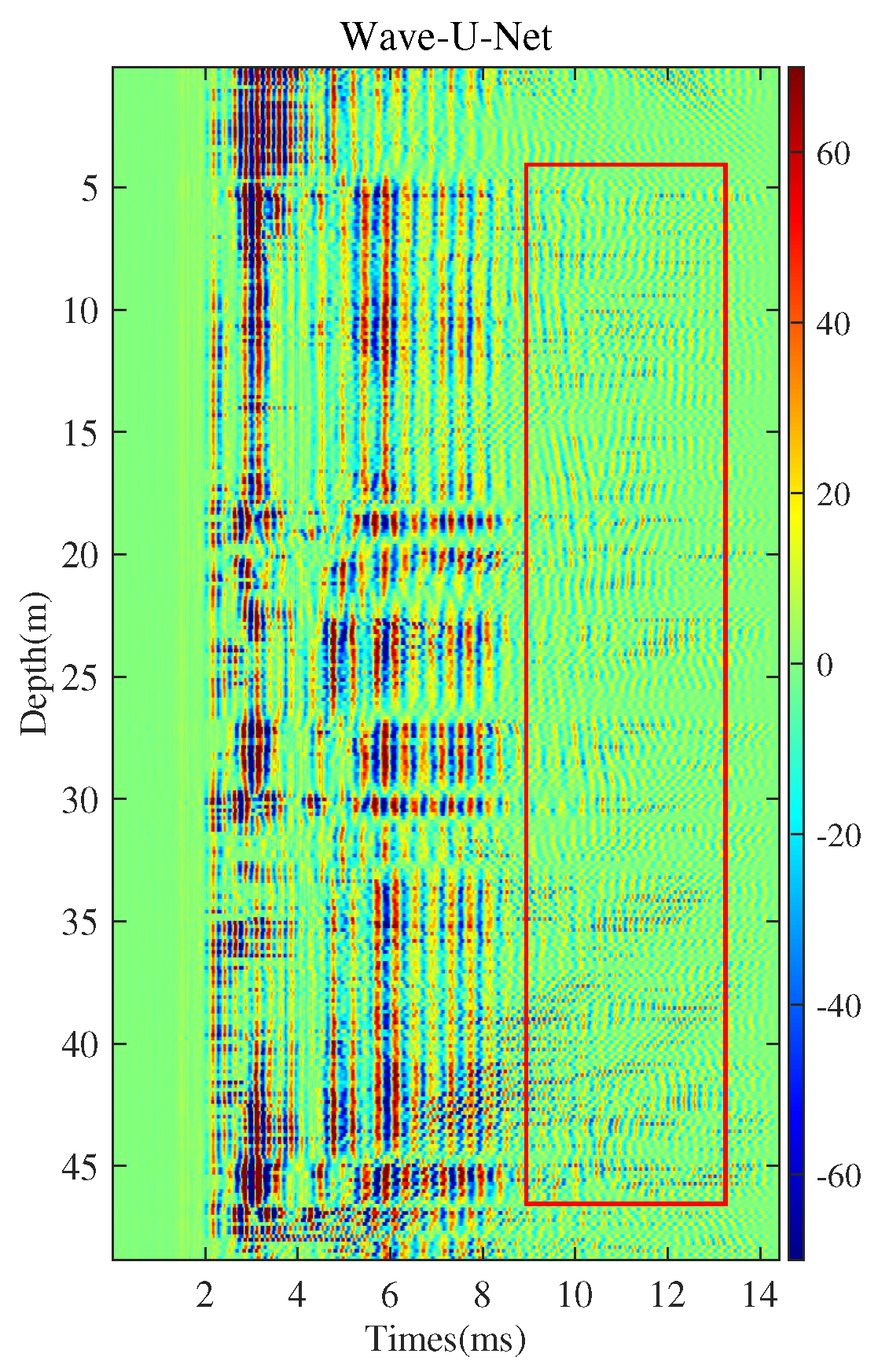
3.6. Comparison of the Wave Separation Capabilities of MC-ConvTasNet and Wave-U-Net

We compare the wave separation performance of MC-ConvTasNet and Wave-U-Net. Wave-U-Net is constructed based on the encoder–decoder architecture proposed in [21], with the encoder comprising four layers. The number of filters doubles in each subsequent layer, specifically totaling 32, 64, 128 and 256. In the decoder, we utilize one-dimensional transposed convolutional layers to replace the upsampling method originally used in the paper. All other details of the Wave-U-Net remain consistent with the description in [21]. After training, the Wave-U-Net achieves a scale-invariant signal-to-noise ratio of 8.7 dB on the test set. Among the three models, namely, the hard-to-hard single-interface model, the soft-to-hard single-interface model and the double-interface model, Wave-U-Net exhibits a lower R std than MC-ConvTasNet. The R std of Wave-U-Net is 23.7 dB, 21.7 dB and 23.7 dB, respectively. In field logging data, the amplitude of the direct wave after suppression using Wave-U-Net is greater than that of MC-ConvTasNet (see Figure 13). Despite having a simpler structure compared to MC-ConvTasNet, Wave-U-Net exhibits an inferior performance and generalization capability when it comes to extracting reflected waves.

4. Discussion

Both the median filter and parameter estimation offer the advantage of simplicity in operation, often allowing for direct use without frequent parameter adjustments in practical applications. However, both methods have their respective limitations. Specifically, the median filter may cause signal distortion and is not applicable to formations parallel to the wellbore axis, while parameter estimation only suppresses the amplitude of direct waves to a certain extent. In contrast, the F-K filter, high-resolution Radon transform and shear wave transform excel in extracting reflected waves from reflectors close to the wellbore. However, they rely on expert experience to adjust method parameters during use, resulting in uncertain required time, and are similarly inapplicable to formations parallel to the wellbore axis. In field logging data, the types of reflectors are often unknown, and each method has its specific limitations. Therefore, when extracting reflected waves, experts often need to judge the possible types of reflectors in each wellbore section based on their experience and select appropriate signal processing methods for extraction. This process is not only time consuming but also inefficient. MC-ConvTasNet overcomes the dependence on expert experience and achieves automatic extraction of reflected waves across the entire wellbore section. Although the performance of MC-ConvTasNet may decline when reflectors are very close to the wellbore, its applicable range still covers the typical distances involved in single-well imaging, ranging from a few meters to several tens of meters.
Although our current research focuses on synthetic data, studies [42,43] have shown that integrating synthetic and real data within datasets can significantly enhance model performance. Therefore, we plan to incorporate partially labeled actual field data into our future work to further improve the robustness of our models. It is recommended that readers first generate synthetic datasets using analytical algorithms to train the neural network. The trained model can then be effectively applied to extract clear reflection waves from field logging data. Subsequently, the reflection waves extracted from each well can be used as known labels to fine-tune the model with field logging data. Through fine-tuning, the model’s generalization capability will be significantly enhanced, thereby further improving its performance in reflection wave extraction.
This paper only focuses on the separation of flexural and reflected waves for dipole S-wave imaging. Further study is being conducted to apply this algorithm to the wave separation of monopole P-wave imaging.

5. Conclusions

We apply MC-ConvTasNet to wave separation to achieve effective extraction of reflected waves. Due to the differences in propagation distance and velocity between the direct and reflected waves, their arrival time differences between channels in the CSG are different. The Conv2d module in MC-ConvTasNet is used to obtain spatial cues between channels to help separate the direct wave and the reflected wave. Because reflectors are rarely known in field logging, synthetic data are used as a dataset in this study. A large number of theoretical waveforms of the CSG are obtained by analytical algorithms.
After training, MC-ConvTasNet exhibits an excellent ability to extract reflected waves. Using three models, we compare the wave separation performance of parameter estimation, MC-ConvTasNet, a median filter and an F-K filter. In the hard-to-hard single-interface model and soft-to-hard single-interface model, the average R std of parameter estimation and the median filter is less than 12.4 dB, less than 31 dB for the F-K filter and more than 33 dB for MC-ConvTasNet. The reflected waves extracted by MC-ConvTasNet are closest to the theoretical reflected waves in both phase and shape, with the largest average R std . In the double-interface model, the average R std of the other three methods is less than 0, while the average R std of MC-ConvTasNet is more than 32 dB. Despite the absence of double-interface samples in the dataset, MC-ConvTasNet exhibits excellent performance in dealing with double-interface cases, and MC-ConvTasNet trained on waveforms in the CSG domain is proven to be suitable for interfaces parallel to the wellbore axis. In the hard-to-hard single-interface model, we compare the wave separation capability of MC-ConvTasNet on waveforms without noise and waveforms with Gaussian white noise. Compared with noise-free data, the increase in the root mean square error is less than 0.06 when the signal-to-noise ratio is 20 dB. MC-ConvTasNet is applicable to data containing noise and maintains good performance.
In the field logging data, MC-ConvTasNet is compared with parameter estimation, a median filter and an F-K filter. Surprisingly, MC-ConvTasNet extracts clearer and more complete reflected waves. The reflector obtained from the imaging of reflected waves extracted by MC-ConvTasNet is the clearest one, with the fewest artifacts, and MC-ConvTasNet achieves both an R dsr and an R snr exceeding 55 dB, demonstrating a superior direct wave suppression capability. Despite the dataset not including field logging data, MC-ConvTasNet is effective for field logging data analysis. When MC-ConvTasNet is used to process the waveforms of the CSG, end-to-end wave separation can be achieved. By inputting the full wave of the CSG containing the currently processed channel, MC-ConvTasNet outputs the time-domain waveforms of direct and reflected waves. It is expected to extract reflected waves in real time when the acoustic logging tool is continuously lifted.

Author Contributions

Conceptualization, data curation, investigation, methodology, software, validation, visualization, writing—original draft, writing—review and editing, W.L.; conceptualization, funding acquisition, resources, writing—review and editing, J.X.; funding acquisition, project administration, supervision, writing—review and editing, H.H. All authors have read and agreed to the published version of the manuscript.

Funding

This work was supported by the National Natural Science Foundation of China (grant no. 12472087, grant no. 42204117, grant no. 12272107).

Institutional Review Board Statement

Not applicable.

Informed Consent Statement

Not applicable.

Data Availability Statement

The original contributions presented in this study are included in the article. Further inquiries can be directed to the corresponding author.

Acknowledgments

We would like to express our sincere gratitude to Xiugang Ma for providing the field logging data, which were essential for the completion of this study. We are also deeply grateful to Yuan Gao for her valuable suggestions during the revision stage of the manuscript, which significantly improved the quality of this paper.

Conflicts of Interest

The authors declare no conflicts of interest.

Abbreviations

The following abbreviations are used in this manuscript:
MC-ConvTasNetMulti-channel convolutional time-domain audio separation network
CSGCommon-source gather
CRGCommon-receiver gather
COGLinear dichroism
Conv-TasNetConvolutional time-domain audio separation network
ICDInter-channel convolution difference
Conv2dTwo-dimensional convolution

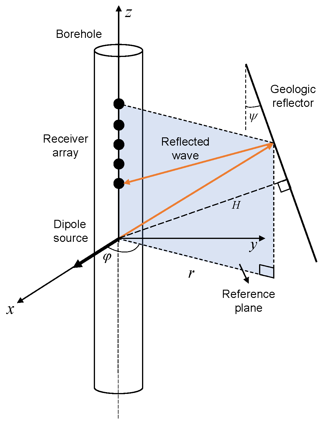
Appendix A. Expressions for Direct and Reflected Waves

Excited by a dipole source along the x-axis, the displacement expression in the fluid is [26]
u 1 = ϕ d + ϕ r ,
where ϕ d and ϕ r are the displacement potentials associated with the source and reflected from the borehole wall, respectively; and ∇ is the Laplacian operator in the cylindrical coordinate system. The displacement potential function in the borehole can be expressed as
ϕ d ( r , φ , z , ω ) = V 0 T ( ω ) 4 π 2 + r 0 f K 1 ( f r ) e j k z cos φ d k , ϕ r ( r , φ , z , ω ) = V 0 T ( ω ) 4 π 2 + r 0 f 2 A ( k , ω ) I 1 ( f r ) e j k z cos φ d k ,
where f 2 = k 2 ω 2 α f 2 ; f and k are the radial wavenumber and axial wavenumber of fluid; w is the angular frequency; α f is the fluid velocity in the borehole; I 1 and K 1 are the first-order modified Bessel function of the first and second kinds, respectively; r 0 is the radius of the dipole source; T ( ω ) represents the spectrum of the time function of the acoustic source; V 0 represents the peak amplitude of the source volume change; φ indicates the azimuth angle; and the coefficient A can be obtained from borehole boundary conditions. The direct wave excited by a dipole source is a flexural wave whose waveform can be calculated by the real axis integration method [27] according to Formula (A1).
Excited by a dipole source along the x-axis, the reflected displacement along the x-axis received in the borehole is [28]
u 2 = u SH + u SV + u P + u SP + u PS ,
where
u S H = T ( ω ) R S H sin 2 φ , u S V = T ( ω ) R S V cos 2 φ , u P = T ( ω ) R P cos 2 φ , u P S = T ( ω ) R P S cos 2 φ , u S P = T ( ω ) R S P cos 2 φ ,
R S H = P 0 R 0 r 0 L ¯ ρ β 2 e j ω L ¯ / β G S H F S H k S θ 1 , ω F S H k S θ 2 , ω , R S V = P 0 R 0 r 0 L ¯ ρ β 2 e j ω L ¯ / β G S V F S V k S θ 1 , ω F S V k S θ 2 , ω , R P = P 0 R 0 r 0 L ¯ ρ α 2 e j ω L ¯ / α G P F P k P θ 1 , ω F P k P θ 2 , ω , R P S = P 0 R 0 r 0 L ˜ S ρ α 2 e j ω L ¯ S / β G P S F P k P θ 1 P , ω F S V k S θ 2 S , ω , R S P = P 0 R 0 r 0 L ˜ P ρ β 2 e j ω L ¯ P / α G S P F S V k S θ 1 S , ω F P k P θ 2 P , ω ,
F P ( k P , ω ) = f C ( k P , ω ) 2 ρ f ω j ρ α , F SH ( k S , ω ) = f D ( k S , ω ) 2 ρ f ω j ρ β sin θ , F SV ( k S , ω ) = f E ( k S , ω ) 2 ρ f ρ sin θ .
Here, u SH , u SV , u P , u SP and u PS are the borehole displacement stimulated by SH-SH, SV-SV, P-P, P-SV and SV-P waves, respectively; R = r 2 + z 2 , k P = ω / α cos θ , k S = ω / β cos θ , cos θ = z / R ; ρ f , ρ , α and β are the fluid density in the borehole, the formation density outside the borehole and the P-wave and S-wave velocities of the formation, respectively; G S H , G S V , G P , G P S and G S P are the plane reflection coefficients of SH-SH, SV-SV, P-P, P-SV and SV-P waves, respectively [31]; L ¯ is the total propagation distance of the reflected wave; L ¯ P and L ¯ S are the distances between the receiver in the borehole and the virtual source of the SV-P and P-SV waves; L ˜ P and L ˜ S are distances associated with the geometric spreading of SV-P and P-SV waves; expressions for L ¯ , L ¯ P , L ¯ S , L ˜ P and L ˜ S can be found in the study of Xu and Hu [28]; θ 1 is the radiation take-off angle of SH-SH, SV-SV and P-P waves from the borehole of the reflected wave; θ 2 is the reception angle of SH-SH, SV-SV and P-P waves upon the borehole of the reflected wave; θ 1 P and θ 1 S represent the incident angle and reflection angle of the P-SV wave relative to the geologic interface, respectively; θ 1 S and θ 2 P represent the incident angle and reflection angle of the SV-P wave relative to the geologic interface, respectively; and the amplitude coefficients C, D and E are obtained by the borehole boundary conditions.

References

  1. Tang, X. Imaging near-borehole structure using directional acoustic-wave measurement. Geophysics 2004, 69, 1378–1386. [Google Scholar] [CrossRef]
  2. Esmersoy, C.; Chang, C.; Kane, M.; Coates, R.; Tichelaar, B.; Quint, E. Acoustic imaging of reservoir structure from a horizontal well. Lead. Edge 1998, 17, 940–946. [Google Scholar] [CrossRef]
  3. Hu, H.; Xu, J.; Wang, Z. Analytical Simulation of the Waves Reflected From a Distant Slanted Interface Outside a Borehole. In Proceedings of the 2019 13th Symposium on Piezoelectrcity, Acoustic Waves and Device Applications (SPAWDA), Shijiazhuang, China, 1–4 November 2019; pp. 1–5. [Google Scholar] [CrossRef]
  4. Xu, J.; Hu, H.; Liu, Q.H. Combination of FDTD with Analytical Methods for Simulating Elastic Scattering of 3-D Objects Outside a Fluid-Filled Borehole. IEEE Trans. Geosci. Remote Sens. 2021, 59, 5325–5334. [Google Scholar] [CrossRef]
  5. Gao, Y.; Hu, H.; Xu, J. Elastic Reverse Time Migration Method for Single-Well Imaging and Elimination of Azimuthal Ambiguity With a Combined Receiver System. IEEE Trans. Geosci. Remote Sens. 2023, 61, 5921215. [Google Scholar] [CrossRef]
  6. Borland, W.; Holderson, J.; Rougha, H.; Sultan, A.; Chakravorty, S.; Al-Raisi, M. Integration of Microelectrical and Sonic Reflection Imaging Around the Borehole-Offshore UAE. In Proceedings of the IPTC International Petroleum Technology Conference, Doha, Qatar, 11 November 2005; p. IPTC-11021. [Google Scholar] [CrossRef]
  7. Hirabayashi, N.; Leaney, W.S. Wavefield separation for borehole acoustic reflection survey using parametric decomposition and waveform inversion. Geophysics 2019, 84, D151–D159. [Google Scholar] [CrossRef]
  8. Tang, X.M.; Zheng, Y.; Patterson, D. Processing array acoustic-logging data to image near-borehole geologic structures. Geophysics 2007, 72, E87–E97. [Google Scholar] [CrossRef]
  9. Hornby, B.E. Imaging of near-borehole structure using full-waveform sonic data. Geophysics 1989, 54, 747–757. [Google Scholar] [CrossRef]
  10. Li, C.; Yue, W. High-resolution Radon transforms for improved dipole acoustic imaging. Geophys. Prospect. 2017, 65, 467–484. [Google Scholar] [CrossRef]
  11. Li, J.; Innanen, K.A.; Tao, G. Extraction of reflected events from sonic-log waveforms using the Karhunen-Loève transform. Geophysics 2017, 82, D265–D277. [Google Scholar] [CrossRef]
  12. Chen, J.; Yue, W.; Li, C.; Zeng, F. Extracting Reflected Waves From Acoustic Logging Data Based on the Shearlet Transform. IEEE Geosci. Remote Sens. Lett. 2019, 16, 1688–1692. [Google Scholar] [CrossRef]
  13. Wang, Q.; Wang, H.; Fang, Z.; Xu, D.; Qi, X.; Yu, Y. Weak Reflection Extraction in Borehole Acoustic Reflection Imaging Using an Unsupervised Machine Learning Method. In Proceedings of the SPWLA Annual Logging Symposium, Rio de Janeiro, Brazil, 18–22 May 2024; SPWLA: Houston, TX, USA, 2024. [Google Scholar]
  14. Li, Y.; Zhou, R.; Tang, X.M.; Jackson, J.; Patterson, D. Single-Well Imaging with Acoustic Reflection Survey at Mounds, Oklahoma, USA. In Proceedings of the 64th EAGE Conference & Exhibition, Florence, Italy, 27–30 May 2002. [Google Scholar] [CrossRef]
  15. Gannot, S.; Vincent, E.; Golan, S.M.; Ozerov, A. A Consolidated Perspective on Multimicrophone Speech Enhancement and Source Separation. IEEE/ACM Trans. Audio Speech Lang. Process. 2017, 25, 692–730. [Google Scholar] [CrossRef]
  16. Hershey, J.R.; Chen, Z.; Le Roux, J.; Watanabe, S. Deep clustering: Discriminative embeddings for segmentation and separation. In Proceedings of the 2016 IEEE International Conference on Acoustics, Speech and Signal Processing (ICASSP), Shanghai, China, 20–25 March 2016; pp. 31–35. [Google Scholar] [CrossRef]
  17. Jansson, A.; Humphrey, E.J.; Montecchio, N.; Bittner, R.M.; Kumar, A.; Weyde, T. Singing Voice Separation with Deep U-Net Convolutional Networks. In Proceedings of the International Society for Music Information Retrieval Conference, Suzhou, China, 23–27 October 2017. [Google Scholar]
  18. Kolbaek, M.; Yu, D.; Tan, Z.; Jensen, J.H. Multitalker Speech Separation With Utterance-Level Permutation Invariant Training of Deep Recurrent Neural Networks. IEEE/ACM Trans. Audio Speech Lang. Process. 2017, 25, 1901–1913. [Google Scholar] [CrossRef]
  19. Wang, D.; Chen, J. Supervised Speech Separation Based on Deep Learning: An Overview. IEEE/ACM Trans. Audio Speech Lang. Process. 2018, 26, 1702–1726. [Google Scholar] [CrossRef] [PubMed]
  20. Luo, Y.; Mesgarani, N. TasNet: Time-Domain Audio Separation Network for Real-Time, Single-Channel Speech Separation. In Proceedings of the 2018 IEEE International Conference on Acoustics, Speech and Signal Processing (ICASSP), Calgary, AB, Canada, 15–20 April 2018; pp. 696–700. [Google Scholar]
  21. Stoller, D.; Ewert, S.; Dixon, S. Wave-U-Net: A Multi-Scale Neural Network for End-to-End Audio Source Separation. arXiv 2018, arXiv:1806.03185. [Google Scholar]
  22. Luo, Y.; Mesgarani, N. Conv-TasNet: Surpassing Ideal Time–Frequency Magnitude Masking for Speech Separation. IEEE/ACM Trans. Audio Speech Lang. Process. 2019, 27, 1256–1266. [Google Scholar] [CrossRef] [PubMed]
  23. Wang, Q.; Wang, H.; Shi, S. A deep learning workflow for weak reflection extraction in pitch-catch measurements in the cased hole. Geophysics 2023, 88, D147–D157. [Google Scholar] [CrossRef]
  24. Gu, R.; Zhang, S.X.; Chen, L.; Xu, Y.; Yu, M.; Su, D.; Zou, Y.; Yu, D. Enhancing End-to-End Multi-Channel Speech Separation Via Spatial Feature Learning. In Proceedings of the ICASSP 2020–2020 IEEE International Conference on Acoustics, Speech and Signal Processing (ICASSP), Barcelona, Spain, 4–8 May 2020; pp. 7319–7323. [Google Scholar] [CrossRef]
  25. Grumiaux, P.A.; Kitić, S.; Girin, L.; Guerin, A. A survey of sound source localization with deep learning methods. J. Acoust. Soc. Am. 2022, 152, 107–151. [Google Scholar] [CrossRef]
  26. Kurkjian, A.L.; Chang, S.K. Acoustic multipole sources in fluid-filled boreholes. Geophysics 1986, 51, 148–163. [Google Scholar] [CrossRef]
  27. Tsang, L.; Rader, D. Numerical evaluation of the transient acoustic waveform due to a point source in a fluid-filled borehole. Geophysics 1979, 44, 1706–1720. [Google Scholar] [CrossRef]
  28. Xu, J.; Hu, H. Solutions of P-SV and SV-P waves in single-well imaging through reciprocity relations. Geophysics 2020, 85, D245–D259. [Google Scholar] [CrossRef]
  29. Luo, Y.; Chen, Z.; Yoshioka, T. Dual-Path RNN: Efficient Long Sequence Modeling for Time-Domain Single-Channel Speech Separation. In Proceedings of the ICASSP 2020–2020 IEEE International Conference on Acoustics, Speech and Signal Processing (ICASSP), Barcelona, Spain, 4–8 May 2020; pp. 46–50. [Google Scholar] [CrossRef]
  30. Tang, X.M.; Cao, J.J.; Wei, Z.T. Shear-wave radiation, reception, and reciprocity of a borehole dipole source: With application to modeling of shear-wave reflection survey. Geophysics 2014, 79, T43–T50. [Google Scholar] [CrossRef]
  31. Aki, K.; Richards, P.G. Quantitative Seismology: Theory and Methods, 2nd ed.; University Science Books: Melville, NY, USA, 2002; pp. 128–149,209–215. [Google Scholar]
  32. Wang, Z.; Hu, H.; Yang, Y. Reciprocity relations for the elastodynamic fields generated by multipole sources in a fluid–solid configuration. Geophys. J. Int. 2015, 203, 883–892. [Google Scholar] [CrossRef]
  33. Xu, J.; Hu, H.; Wang, Z. Asymptotic solution to a 3D dipole single-well imaging system with combined monopole and dipole receivers with an application in elimination of azimuth ambiguity. Geophysics 2019, 84, D191–D207. [Google Scholar] [CrossRef]
  34. Castagna, J.P.; Batzle, M.L.; Eastwood, R.L. Relationships between compressional-wave and shear-wave velocities in clastic silicate rocks. Geophysics 1985, 50, 571–581. [Google Scholar] [CrossRef]
  35. Li, Q. Velocity regularities of p and s-waves in formations. Oil Geophys. Prospect. (China) 1992, 27, 5519369. [Google Scholar]
  36. Ma, Z.; Xie, J. Relationship among conpressional wave, shear wave velocities and density in rocks. Prog. Geophys. 2005, 20, 905–910. [Google Scholar]
  37. Kolbæk, M.; Tan, Z.; Jensen, S.H.; Jensen, J.H. On Loss Functions for Supervised Monaural Time-Domain Speech Enhancement. IEEE/ACM Trans. Audio Speech Lang. Process. 2019, 28, 825–838. [Google Scholar] [CrossRef]
  38. Roux, J.L.; Wisdom, S.; Erdogan, H.; Hershey, J.R. SDR—Half-baked or Well Done? In Proceedings of the ICASSP 2019—2019 IEEE International Conference on Acoustics, Speech and Signal Processing (ICASSP), Brighton, UK, 12–17 May 2019; pp. 626–630. [Google Scholar] [CrossRef]
  39. Kingma, D.P.; Ba, J. Adam: A Method for Stochastic Optimization. arXiv 2014, arXiv:1412.6980. [Google Scholar]
  40. Gazdag, J.; Sguazzero, P. Migration of seismic data by phase shift plus interpolation. Geophysics 1984, 49, 124–131. [Google Scholar] [CrossRef]
  41. Sridhar, K.; Cutler, R.; Saabas, A.; Parnamaa, T.; Loide, M.; Gamper, H.; Braun, S.; Aichner, R.; Srinivasan, S. ICASSP 2021 Acoustic Echo Cancellation Challenge: Datasets, Testing Framework, and Results. In Proceedings of the ICASSP 2021—2021 IEEE International Conference on Acoustics, Speech and Signal Processing (ICASSP), Toronto, ON, Canada, 6–11 June 2021; pp. 151–155. [Google Scholar] [CrossRef]
  42. Zhu, W.; Mousavi, S.M.; Beroza, G.C. Chapter Four—Seismic signal augmentation to improve generalization of deep neural networks. In Machine Learning in Geosciences; Advances in Geophysics; Moseley, B., Krischer, L., Eds.; Elsevier: Amsterdam, The Netherlands, 2020; Volume 61, pp. 151–177. [Google Scholar] [CrossRef]
  43. Yan, Z.; Zhang, Z.; Liu, S. Improving Performance of Seismic Fault Detection by Fine-Tuning the Convolutional Neural Network Pre-Trained with Synthetic Samples. Energies 2021, 14, 3650. [Google Scholar] [CrossRef]
Figure 1. Dipole shear wave imaging schematic diagram. The logging tool is positioned at the center of the wellbore, with its dipole source responsible for exciting the signal. This signal is then captured by a receiver array consisting of eight receivers. This receiver array is capable of not only receiving direct waves propagating along the wellbore but also capturing reflected waves returned from the reflector located near the wellbore. The blue arrow indicates the propagation path of the direct wave, while the black arrow represents the propagation path of the reflected wave.
Applsci 15 04189 g001
Figure 2. MC-ConvTasNet model flow chart. The process of the MC-ConvTasNet model is introduced using channel 1 as the currently processed channel. ⊕ represents concatenation of the output features of the encoder and Conv2d. ⊙ represents calculation of the Hadamard product of the outputs of the encoder and separator. w represents an encoded representation of a full wave. m i , i = 1 , 2 represents a mask of a direct wave or a reflected wave. d i , i = 1 , 2 represents an encoded feature representation of a direct wave or a reflected wave.
Applsci 15 04189 g002
Figure 3. The schematic diagram for segmentation and mapping of the encoder and the schematic diagram for mapping and overlapping addition of the decoder. (a) shows that the full wave is divided into overlapping segments. (b) shows that the encoder converts a full wave segment x to an encoded representation w . (c) shows that the decoder converts an encoded feature representation of a direct wave or a reflected wave d i to a time-domain segment x ^ i . (d) shows that, by performing overlapping addition on segments in a block, the output of the decoder is converted back to a sequential output.
Applsci 15 04189 g003
Figure 4. Conceptual illustration of the ICD generation process. The first element of the ICD matrix is obtained by the Hadamard product of the shadow matrix in y with the convolution kernel K and then calculating the dot product with the window function h . B represents the number of 2-D convolution kernels (or the number of filters). The image is adapted from Figure 4 in the study of Gu et al. [24], to maintain consistency with Equation (9).
Applsci 15 04189 g004
Figure 5. Illustration of geometric characteristic parameters for a single reflector. A dipole source is placed along the x-axis of the Cartesian coordinate ( x , y , z ) . The cylindrical coordinate ( r , z , φ ) is also shown in the figure. ψ is the dip angle of the reflector relative to the wellbore axis. H is the distance from the source to the reflector. φ is the azimuth of the reflector.
Applsci 15 04189 g005
Figure 6. Forward calculation model. (a) is a schematic diagram of the single-interface model containing interface 1. (b) is the top view of the double-interface model. (c,d) are, respectively, schematic diagrams of interface 2 and interface 3 in the double-interface model.
Applsci 15 04189 g006
Figure 7. Full waveforms and extracted reflected waves for the hard-to-hard single-interface model. (a,b) are, respectively, COG full waveforms and reflected waveforms obtained by forward simulation. (cf) are the reflected waves separated by parameter estimation, MC-ConvTasNet, median filter and F-K filter, respectively. (a,c) are normalized by the maximum amplitude of the flexural wave. The rest are normalized by the maximum amplitude of the reflected wave. The average R std for parameter estimation, MC-ConvTasNet, the median filter and the F-K filter is −24.9 dB, 34.7 dB, 6.8 dB and 27.9 dB, respectively.
Applsci 15 04189 g007aApplsci 15 04189 g007b
Figure 8. Full waveforms and extracted reflected waves for the soft-to-hard single-interface model. (a,b) are, respectively, COG full waveforms and reflected waveforms obtained by forward simulation. (cf) are the reflected waves separated by parameter estimation, MC-ConvTasNet, median filter and F-K filter, respectively. (a,c) are normalized by the maximum amplitude of the flexural wave. The rest are normalized by the maximum amplitude of the reflected wave. The average R std for parameter estimation, MC-ConvTasNet, the median filter and the F-K filter is −25.7 dB, 33.4 dB, 12.4 dB and 30.6 dB, respectively.
Applsci 15 04189 g008aApplsci 15 04189 g008b
Figure 9. Full waveforms and extracted reflected waves for the double-interface model. (a,b) are, respectively, COG full waveforms and reflected waveforms obtained by forward simulation. (ce) are the reflected waves separated by MC-ConvTasNet, median filter and F-K filter, respectively. On trace 1 in (b), the arrivals are a reflected S-wave from interface 2 (red solid line), a reflected P-wave (blue dashed line), a converted wave (green dashed line) and a reflected S-wave (yellow dashed line) from interface 3. The average R std for MC-ConvTasNet, the median filter and the F-K filter is 32.3 dB, −19.1 dB and −19.5 dB, respectively.
Applsci 15 04189 g009
Figure 10. Full waveforms and extracted reflected waves for the double-interface model. (a,b) are, respectively, the full waveform and the reflected waveform of the CSG at a depth of 6 inches. (c,d) are the reflected waves separated by MC-ConvTasNet and parameter estimation, respectively. (a,c) are normalized with the maximum amplitude of the flexural wave. (b,d) are normalized with the maximum amplitude of the reflected wave. The average R std for parameter estimation and MC-ConvTasNet is −25.0 dB and 32.3 dB, respectively.
Applsci 15 04189 g010aApplsci 15 04189 g010b
Figure 11. Full waveforms containing noise and extracted reflected waves for the hard-to-hard single-interface model. (a,d) are COG full waveforms containing Gaussian white noise with signal-to-noise ratios of 20 dB and 25 dB, respectively. (b,e) are the reflected waves separated by MC-ConvTasNet. Trace 4 in (b,e) is compared with the full wave and the theoretical reflected wave, respectively, as shown in (c,f). The R rmse for 20 dB and 25 dB is 0.100 and 0.0649, respectively.
Applsci 15 04189 g011aApplsci 15 04189 g011b
Figure 12. The reflected waves extracted from field logging data. (a) is a COG variable density map of field logging data. (be) are COG variable density maps of the reflected waves extracted by parameter estimation, the median filter, the F-K filter and MC-ConvTasNet, respectively. In each of these maps, the area containing the reflected waves is highlighted with a solid red box. (fi) are imaging results of reflected waves extracted by these four methods, respectively. In each of these maps, the area the reflector is highlighted with a dotted red box. The values displayed in the variable density maps (ah) are clipped to a range of +/−70. The values displayed in the variable density map (i) are clipped to a range of +/−250.
Applsci 15 04189 g012
Figure 13. Reflection waves extracted from field logging data by Wave-U-Net. The area containing the reflected waves is highlighted with a solid red box. The values displayed in the variable density map are clipped to a range of +/−70.
Applsci 15 04189 g013
Table 1. Variation range of the geometric characteristics of reflectors in the dataset.
Geometry PropertiesLower LimitUpper LimitStep Size
Distance (m)3131
Dip angle (°)−707010
Azimuth angle (°)09045
Table 2. Variation range of parameters of formations on both sides of the reflector in the dataset.
Formation ParametersLower LimitUpper Limit
P-velocity (m/s)25955080
S-velocity (m/s)11703200
Density ( kg / m 3 )17432702
Table 3. The formation parameters in reflector models.
ModelP-Velocity (m/s)S-Velocity (m/s)Density ( kg / m 3 )
Fluid1500-1000
Formation 1300018002000
Formation 2220012002000
Formation 3450024002650
Table 4. Average R std of four methods over three models.
Model R std (dB)
MC-ConvTasNetMedian FilterParameter EstimationF-K Filter
134.76.8−24.927.9
233.412.4−25.730.6
332.3−19.1−25.0−19.5
Table 5. Average R rmse of four methods over three models.
Model R rmse (dB)
MC-ConvTasNetMedian FilterParameter EstimationF-K Filter
10.0440.0772.0800.006
20.0100.0301.8930.003
30.0280.1332.1460.133
Disclaimer/Publisher’s Note: The statements, opinions and data contained in all publications are solely those of the individual author(s) and contributor(s) and not of MDPI and/or the editor(s). MDPI and/or the editor(s) disclaim responsibility for any injury to people or property resulting from any ideas, methods, instructions or products referred to in the content.

