The 3D Gaussian Splatting SLAM System for Dynamic Scenes Based on LiDAR Point Clouds and Vision Fusion

Abstract

This paper presents a novel 3D Gaussian Splatting (3DGS)-based Simultaneous Localization and Mapping (SLAM) system that integrates Light Detection and Ranging (LiDAR) and vision data to enhance dynamic scene tracking and reconstruction. Existing 3DGS systems face challenges in sensor fusion and handling dynamic objects. To address these, we introduce a hybrid uncertainty-based 3D segmentation method that leverages uncertainty estimation and 3D object detection, effectively removing dynamic points and improving static map reconstruction. Our system also employs a sliding window-based keyframe fusion strategy that reduces computational load while maintaining accuracy. By incorporating a novel dynamic rendering loss function and pruning techniques, we suppress artifacts such as ghosting and ensure real-time operation in complex environments. Extensive experiments show that our system outperforms existing methods in dynamic object removal and overall reconstruction quality. The key innovations of our work lie in its integration of hybrid uncertainty-based segmentation, dynamic rendering loss functions, and an optimized sliding window strategy, which collectively enhance robustness and efficiency in dynamic scene reconstruction. This approach offers a promising solution for real-time robotic applications, including autonomous navigation and augmented reality.

1. Introduction

With the advancement of Simultaneous Localization and Mapping (SLAM) [1,2,3,4,5,6,7], SLAM systems oriented towards multi-sensor fusion are gaining prominence in robotic perception, applications, and embodied intelligence as well as in motion control. Dense SLAM, which integrates LiDAR and visual sensors, has attracted significant attention over sparse SLAM due to its superior scene reconstruction capabilities and its potential for semantic segmentation. Real-time dense SLAM systems capable of reconstructing high-fidelity models with rich texture details are crucial for enhancing the comprehensive capabilities of robotic systems, particularly in complex and dynamic environments where accurate 3D reconstructions are essential for effective navigation, interaction, and task execution. The fusion of LiDAR and visual data allows systems to leverage the complementary strengths of both sensor types, where LiDAR provides precise depth measurements and visual sensors offer rich color and texture information.

Recently, 3D Gaussian Splatting (3DGS) has demonstrated significant performance in multi-view high-fidelity reconstruction and rapid rendering, leading to the emergence of 3DGS-based SLAM systems [8,9,10,11,12]. 3DGS has proven to be particularly effective in scenarios that require fine details, such as in environments with complex structures, dynamic scenes, and large-scale maps. However, existing 3DGS-SLAM systems face two major challenges that significantly affect their practical utility. First, most of these systems focus on single-sensor setups such as LiDAR or RGB/RGB-D cameras, and lack effective sensor fusion techniques that would enable them to fully exploit the strengths of each sensor modality. While individual sensors such as LiDAR or cameras can provide valuable data, combining them in a meaningful way remains an open challenge in real-world environments. Second, these systems struggle with the dynamic objects commonly encountered in real-world environments. Dynamic objects such as moving vehicles, pedestrians, and other obstacles introduce significant errors in pose estimation and cause map reconstruction artifacts. In certain cases, dynamic interference can lead to complete failure in scene reconstruction, making the SLAM system unreliable for critical applications such as autonomous driving, robotics in indoor environments, and augmented reality.

To address these challenges, this paper proposed a novel 3DGS-based SLAM system which effectively integrates the multiple sensor modalities of LiDAR and vision for enhanced robustness against dynamic interference and improved dynamic object removal. Our key innovation lies in the integration of a hybrid uncertainty-based 3D segmentation method, a dynamic rendering loss function, and a sliding window-based keyframe fusion strategy. Dynamic interference, particularly in the case of LiDAR, primarily occurs during point-cloud initialization, where moving objects may be incorrectly incorporated into the 3D map. To mitigate this, we introduce a point cloud segmentation strategy that leverages visual uncertainty estimation and 3D object detection techniques to identify and eliminate dynamic points from the point cloud. Additionally, we apply uncertainty-based segmentation to the Gaussian components, effectively removing dynamic points from the 3D Gaussian scene representation. This dynamic object removal strategy ensures that the system maintains a high level of accuracy in static map reconstruction even in the presence of moving objects.

To further improve the proposed system’s ability to handle dynamic environments, we introduce a keyframe fusion strategy based on a sliding window optimization approach. This method minimizes the Gaussian rendering loss by selectively fusing keyframes that provide complementary information from both LiDAR and visual inputs. The sliding window optimization ensures that the most relevant frames are considered, thereby reducing computational overhead while maintaining reconstruction accuracy. In addition, we apply dynamic loss functions and point cloud initialization pruning to suppress reconstruction artifacts such as smearing or ghosting effects caused by dynamic objects. These enhancements ensure that the system is not only accurate but also efficient and capable of operating in real-time even in complex and dynamic environments.

Experimental results demonstrate that our approach effectively removes dynamic interference, accurately recovers camera poses, and supports multi-sensor input for robust scene tracking and reconstruction. The proposed fusion framework minimizes both computational and memory overhead, enabling real-time rendering and efficient processing. Our system outperforms existing state-of-the-art 3DGS-SLAM methods in terms of dynamic object handling and overall reconstruction quality, making it a promising solution for real-world robotic applications.

The key contributions of our work are summarized as follows:

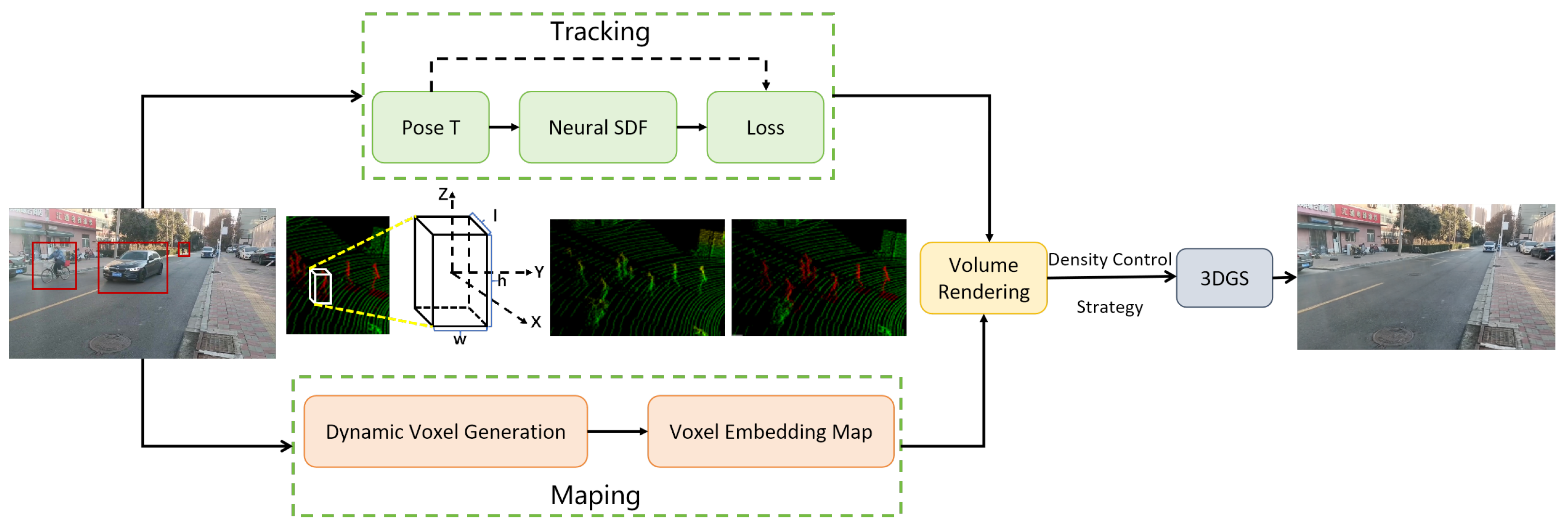
• A 3DGS-SLAM system designed specifically for dynamic environments, incorporating tracking, 3D segmentation, and mapping threads to enable real-time dynamic scene tracking and reconstruction with both vision and LiDAR inputs. This system addresses key challenges in dynamic scene reconstruction and improves the robustness of SLAM in real-world environments.
• A hybrid uncertainty-based 3D segmentation method accurately segments dynamic LiDAR point clouds and effectively removes uncertain dynamic points at the boundaries. This method ensures that moving objects and other uncertainties do not interfere with the static map reconstruction.
• A dynamic rendering loss function and a sensor-fusion-based keyframe selection strategy ensure accurate removal of dynamic artifacts while minimizing computational overhead. This approach allows the system to operate in real time, even in large-scale and highly dynamic environments.
• Evaluation of our approach on multiple public and in-house real-world datasets demonstrates superior performance across multiple metrics, achieving high-fidelity reconstruction and effective dynamic interference removal. Our system consistently outperforms existing methods in both dynamic object handling and overall map quality.

2. Related Work

Current SLAM systems primarily focus on improving the accuracy of reconstruction using visual sensors. Methods based on monocular, stereo, and RGB-D cameras have achieved significant progress in creating dense and detailed environmental maps. However, visual sensors often perform poorly in environments with low lighting, textureless surfaces, or dynamic objects, limiting their applicability in real-world scenarios. In contrast, LiDAR (Light Detection and Ranging), with its millimeter-level positioning accuracy and adaptability to diverse environments, plays a crucial role in SLAM systems. LiDAR excels in capturing precise depth information, particularly in large-scale and unbounded environments, making it an indispensable component in fields such as autonomous driving and robotics.

To overcome this limitation, recent research has attempted to leveraging the complementary strengths of both modalities by combining visual data with LiDAR data. Among these efforts, 3DGS-based LiDAR–Visual fusion and NeRF-based LiDAR–Visual fusion have emerged as two critical research directions. The following sections discuss the relevant work in these two areas in detail.

2.1. NeRF-Based LiDAR–Visual Fusion

Several NeRF-SLAM systems have begun to explore the integration of visual and LiDAR data to enhance the quality of 3D scene reconstruction. For instance, NeRF-LOAM [13] introduces a neural Signed Distance Function (SDF) to classify LiDAR point clouds into ground and non-ground points, effectively reducing Z-axis drift. It also simultaneously optimizes odometry and voxel embeddings to generate dense and smooth environmental mesh maps, addressing the limitations of traditional methods in large-scale scenes. LONER [14] employs LiDAR data to train a Multi-Layer Perceptron (MLP) for estimating dense maps and sensor trajectories. By incorporating a novel information-theoretic loss function, it optimizes the online training process to achieve faster convergence and higher geometric reconstruction accuracy than other deep-supervised neural implicit frameworks. However, it still faces challenges in dynamic object removal and void filling. PIN-SLAM [15] leverages an implicit neural network representation of elastic point clouds to construct globally consistent large-scale maps without relying on GPS, Inertial Measurement Units (IMUs), or wheel odometry. Using approximately 20,000 LiDAR scans, it improves map accuracy and consistency; however, its reconstruction quality is constrained by the fixed resolution of the neural points. CLONeR [16] is an occupancy-grid-assisted neural representation that integrates camera and LiDAR data by decoupling the learning of occupancy information and color representation. By using separate MLPs for training with LiDAR and camera data, CLONeR enhances NeRF’s performance in large-scale unbounded outdoor scenes, especially in sparse-view settings.

2.2. 3DGS-Based LiDAR–Visual Fusion

Integrating LiDAR data has greatly improved the effectiveness of 3D Gaussian Splatting (3DGS) for large-scale scene reconstruction. 3DGS-ReLoc [17] and Gaussian-LIC [18] leverage LiDAR point clouds along with associated images to generate 3D maps, resulting in more detailed environmental modeling. Similarly, DrivingGaussian [19] enhances the integration of features by extracting image information and projecting combined LiDAR scans. LetsGo [20] integrates Level-of-Detail (LoD) rendering into 3DGS workflows, offering an efficient way to represent scenes using Gaussian functions at varying resolutions. LIV-GaussianMap [21] increases the efficiency of managing point clouds by utilizing a well-structured explicit octree, while TCLC-GS [22] applies a hierarchical octree of implicit feature grids and further optimizes 3DGS through advanced color projection methods. MM-Gaussian [23] employs point cloud registration to estimate camera poses and incorporates these point clouds into maps, which improves optimization. This approach also supports progressive map visualization and leverages high-fidelity scene reconstructions to refine poses, resulting in improved positioning accuracy and mapping quality. LiV-GS [24] refines pose estimation by aligning Gaussian covariance matrices with current observations and enhances efficiency through backend corrections and Gaussian map updates. Additionally, it addresses challenges in depth continuity within unbounded environments by employing a LiDAR-based Gaussian splitting mechanism, significantly boosting performance and positioning accuracy in extensive outdoor scenarios.

However, most of the aforementioned methods assume static environments and have limited ability to handle dynamic scenes. In dynamic scenarios, moving objects, feature matching errors, or tracking loss can significantly degrade reconstruction accuracy. To address these challenges, in this paper we propose a 3DGS-SLAM method that resists dynamic interference, helping to achieve high-precision 3D map construction in dynamic environments.

3. Methodology

The architecture of the multi-sensor fusion SLAM system presented in this paper is shown in Figure 1. It consists of three core modules: the segmentation module, tracking module, and Gaussian mapping module. The 3D segmentation module is employed to initially filter out laser point clouds corresponding to dynamic human bodies, while visual uncertainty segmentation is used to eliminate dynamic points at the edges, thereby enhancing segmentation robustness. The tracking module operates synchronously in a separate thread, continuously updating laser tracking results and extracting visual keyframes for high-fidelity reconstruction. The Gaussian mapping module utilizes laser point clouds for initialization and keyframes for mapping, incorporating a unique dynamic loss function in the mapping process. By seamlessly integrating these three modules, the system’s operational efficiency is enhanced and its memory usage is reduced. An example result is provided to demonstrate the performance of the end-to-end system.

3.1. Foreground–Background Segmentation

Traditional foreground–background segmentation typically operates at the 2D level. In contrast, we perform segmentation using both LiDAR-based and visual 3D bounding boxes, defining dynamic human bodies as the foreground and all other objects as the background. The moving objects in the scene, denoted as $\{O_N,\dots ,O_M\}={\left\{O_i\right\}}_{i=N}^M$, are tracked and enclosed within 3D bounding boxes, represented by the set $\{B_N,\dots ,B_M\}={\left\{B_i\right\}}_{i=N}^M$. As illustrated in Figure 2, each bounding box $B_i=\{P_{ci},h_i,w_i,l_i\}$, where $P_{ci}={\{x_{ci},y_{ci},z_{ci}\}}^T$ represents the center coordinates of the 3D bounding box $B_i$, with $h_i$, $w_i$, and $l_i$ corresponding to its height, width, and length, respectively, and the subscript i referring to the specific object.

To achieve this goal, we maintain a global dynamic list L in which each element corresponds to the dynamic mask $D_i$ of a moving object $O_i$. This list is defined as $L={\left\{D_i\right\}}_{i=N}^M$, representing the masks of all detected moving objects. The mask $D_i=\{p_{li},p_{ri}\}$ is defined as follows:

$$p_{i1}=\left({\left(R{P}_i\right)}_x+T_x-{\displaystyle \frac{w_i}{2}},{\left(R{P}_i\right)}_y+T_y-{\displaystyle \frac{l_i}{2}}\right),$$

(1)

$$p_{i2}=\left({\left(R{P}_i\right)}_x+T_x+{\displaystyle \frac{w_i}{2}},{\left(R{P}_i\right)}_y+T_y+{\displaystyle \frac{l_i}{2}}\right),$$

(2)

where R and T represent rotation and translation, respectively, with R being the rotation matrix and T the translation vector. Based on this, we optimize the detection process by incorporating weight assessments for points within dynamic object masks. We utilize a deep learning-based visual model such as Mask R-CNN or PointPillars for 3D segmentation, generating the visual segmentation mask $V_i$. We then fuse the visual segmentation mask $V_i$ with the LiDAR segmentation mask $D_i$ to form the composite mask $C_i$:

$$C_i=D_i\cup V_i.$$

(3)

To enhance this process, we introduce a distance-based dynamic weight $w_{\mathrm{dyn}}\left(p\right)$ for the existing mask representation $D_i=\{p_{li},p_{ri}\}$. For each point p in the mask $D_i$, we apply a dynamic weight based on the point’s distance $D\left(p\right)$ to the 3D box. Let $D_{\max }$ denote the maximum size or reference distance of the 3D box. The distance $D\left(p\right)$ from point p to the interior of the box is used to adjust the point’s weight. The closer the point to the box, the higher the weight, indicating a higher likelihood of it being dynamic; conversely, the farther the distance, the lower the weight, suggesting a higher likelihood of it being static. The adjustment formula is provided by

$$w_{\mathrm{dyn}}\left(p\right)=1-{\displaystyle \frac{D\left(p\right)}{D_{\max }}}.$$

(4)

Next, we calculate the comprehensive weight $W\left(p\right)$ for each point in the mask, considering both the point’s occupancy rate $\varphi \left(p\right)$ and its dynamic weight $w_{\mathrm{dyn}}\left(p\right)$:

$$W\left(p\right)=\varphi \left(p\right)·w_{\mathrm{dyn}}\left(p\right).$$

(5)

Based on the comprehensive weight $W\left(p\right)$, we determine whether to retain or remove a point according to a predefined threshold.

For each point p in the composite mask $C_i$, we calculate its comprehensive weight $W\left(p\right)$ by considering both its dynamic weight $w_{\mathrm{dyn}}\left(p\right)$ and its uncertainty weight $w_{\mathrm{unc}}\left(p\right)$:

$$W\left(p\right)=\varphi \left(p\right)·w_{\mathrm{dyn}}\left(p\right)·w_{\mathrm{unc}}\left(p\right)$$

(6)

where $\varphi \left(p\right)$ is the occupancy rate of point p.

Based on the comprehensive weight $W\left(p\right)$, we determine whether to retain or remove a point according to a predefined threshold $\theta$. If $W\left(p\right)>\theta$, then the point is considered dynamic and is removed from the static background reconstruction; otherwise, it is retained as part of the static background.

To update the dynamic list L, we remove elements whenever a new frame arrives based on $y_{ci}$. If $y_{ci}<T_y$, then the corresponding element is removed from the list. Therefore, when a new frame is input, if a LiDAR point is both non-ground and falls within any mask in the list $L={\left\{C_i\right\}}_{i=N}^M$, these points are considered part of the dynamic foreground and are not included in the static background reconstruction. The method for determining whether a LiDAR point is a ground point follows the approach outlined in [13].

When processing dynamic foreground regions, our method assumes that only the ground surface G needs to be generated within these areas. However, completely ignoring dynamic objects may lead to gaps in the ground surface reconstruction. To address this, we first calculate the average ground height ${\overline{z}}_G$ along the z-axis within a radius r around the composite mask $C_i$. The average height is computed as

$${\overline{z}}_G={\displaystyle \frac{1}{|P_G|}}\sum _{p\in {\mathcal{P}}_G}{z}_p,$$

(7)

where $P_G$ is the set of ground points within radius r around $C_i$ and $z_p$ is the z-coordinate of each point in $P_G$.

To ensure continuity of the ground surface, we generate artificial LiDAR points $\widehat{P_G}=\{\widehat{p_1},\widehat{p_2},\dots ,\widehat{p_n}\}$ at the estimated height ${\overline{z}}_G$. These points $\widehat{p_j}$ satisfy

$${\widehat{p}}_j=(x_j,y_j,{\overline{z}}_G),j=1,2,\dots ,n,$$

(8)

where $(x_j,y_j)$ are randomly sampled within $C_i$. These artificially generated points $\widehat{p_j}$ are then incorporated into the reconstruction process.

For each point p in the composite mask $C_i$, we calculate its uncertainty; if a point is classified inconsistently between the LiDAR segmentation and the visual segmentation (i.e., marked as dynamic by one method and static by the other), then it is labeled as uncertain. To represent the degree of uncertainty, we introduce an uncertainty weight $w_{\mathrm{unc}}\left(p\right)$ ranging from 0 to 1:

$$w_{\mathrm{unc}}\left(p\right)=\left\{\begin{array}{cc}1,\hfill & \mathrm{if}\mathrm{consistent}\mathrm{in}{D}_i\mathrm{and}{V}_i\hfill \\ \alpha ,\hfill & \mathrm{if}\mathrm{inconsistent}\mathrm{in}{D}_i\mathrm{and}{V}_i\hfill \end{array}\right.$$

(9)

where $\alpha$ is a parameter between 0 and 1 that represents the degree of uncertainty, which can be adjusted as needed. In this study, we set $\alpha =0.9$.

3.2. Sliding Window-Based Reconstruction Strategy

To effectively mitigate the interference of dynamic objects on static background reconstruction, we propose a sliding-window-based dynamic background restoration strategy. In dynamic scenes, object motion often generates artifacts which disrupt accurate background reconstruction, particularly under motion blur. Artifacts such as incorrect depth or color information in regions affected by moving objects can severely impact the quality of static scene reconstruction. To address this, we aggregate consecutive frame data into sliding windows, with each window containing w frames. This sliding window mechanism allows for more robust identification and removal of artifacts caused by dynamic objects by leveraging the temporal and spatial relationships across frames. The use of multiframe data not only enhances the accuracy of static background restoration but also improves the continuity of the reconstruction by minimizing the impact of transient dynamic objects that might otherwise cause disruptions.

In our approach, we begin by performing intraframe consistency checks within each frame of the sliding window. Specifically, we calculate the depth and color differences between adjacent pixels in each frame. If the depth or color variations within a specific region exceed preset thresholds, then this region is marked as a dynamic candidate. These thresholds (${\tau }_d$ for depth and ${\tau }_c$ for color) are critical for distinguishing between static and dynamic elements in the scene. These dynamic candidate regions are then subjected to further verification to determine whether they are indeed caused by dynamic objects.

After potential dynamic regions have been identified, we track their changes over multiple frames within the sliding window. This tracking is essential for distinguishing between transient changes such as those caused by dynamic objects and permanent scene elements caused by static objects. We examine changes in the position, shape, and appearance of these regions over consecutive frames, which can provide a more accurate classification of their dynamic nature. For regions confirmed to be dynamic, we apply a spatiotemporal consistency-based background restoration algorithm. This algorithm reconstructs the background occluded by dynamic objects by aggregating static information from corresponding positions in other frames within the sliding window. The weighted averaging process considers both the temporal distance (time difference) and spatial distance (distance in pixel space), with the following weight function:

$$w(p,t)=exp(-\alpha |t-t_c\left|\right)·exp(-\beta |p-p_c\left|\right)$$

(10)

where $t_c$ is the current frame time, $p_c$ is the position of the point to be restored, and $\alpha$ and $\beta$ are temporal and spatial decay factors, respectively. These weights ensure that more recent and closer frames contribute more significantly to the reconstruction, making the restoration process more accurate and coherent. By aggregating data from multiple frames, this algorithm can accurately reconstruct background regions occluded by dynamic objects, allowing for enhanced scene fidelity and continuity.

To ensure smooth transitions between adjacent sliding windows, we adopt a 50% overlap strategy. This strategy mitigates the potential for visible seams or discontinuities between windows by blending the overlapping regions. The linear weight fusion used in this process is described by the following formula:

$$I_{final}=w_1{I}_{window1}+w_2{I}_{window2}$$

(11)

where $w_1$ and $w_2$ are position-related linear weights satisfying $w_1+w_2=1$. This overlapping and fusion strategy is vital for maintaining continuity in the reconstructed scene, which ensures that the transitions between consecutive windows are seamless and visually coherent. The overlap also helps to reduce the risk of missing or misrepresenting static regions that may occur at the boundary of sliding windows.

The sliding window-based reconstruction strategy significantly improves the overall quality of dynamic scene reconstruction, particularly in complex environments where dynamic objects constantly interfere with static background reconstruction. The ability of this strategy to aggregate information across multiple frames helps in handling both small-scale and large-scale dynamic interference. The accuracy of the background restoration is further enhanced by the use of temporal and spatial weighting, which ensures that the most relevant frames are prioritized during the reconstruction process. Moreover, the sliding window approach ensures that dynamic objects are effectively suppressed without sacrificing the accuracy or completeness of the static scene.

Algorithm 1 provides the pseudocode for the sliding window-based reconstruction strategy, outlining the key steps involved in the dynamic background restoration process. It highlights the iterative nature of the approach, through which each window of frames is processed sequentially, dynamic regions are verified, and static regions are reconstructed. The use of weighted averaging in the background restoration step ensures that the final result accurately reflects the static scene without artifacts caused by dynamic interference.

3.3. 3DGS-Based Dense Scene Representation

To optimize the scene representation, we adopt 3D Gaussian Splatting (3DGS) as the map primitive for high-quality scene reconstruction and novel view synthesis. 3DGS models the scene as a set of Gaussian primitives distributed in 3D space, leveraging differentiable rendering techniques to achieve image reconstruction and scene optimization for given viewpoints. This representation allows for continuous and smooth blending of 3D structures, making it well suited for dynamic environments where precise reconstruction is critical. Although dynamic 3D points are eliminated during initialization to reduce the system’s dependence on segmentation methods, we incorporate dynamic mapping points during the 3DGS training phase to suppress their impact on reconstruction results. This dynamic adjustment ensures that the final reconstruction is not distorted by moving objects or noisy data. Additionally, we introduce a curling loss function to constrain edge projections and further enhance reconstruction accuracy by preserving fine geometric details, particularly in scenes with complex structures or occlusions.

Algorithm 1 Sliding Window-Based Dynamic Scene Reconstruction

Require:  Frame sequence $F=\{f_1,f_2,\dots ,f_n\}$, window size w, overlap ratio r  Ensure:  Reconstructed static scene S 1: Initialize $S=\varnothing$, window stride $s=w\times (1-r)$ 2: for $i=1$ to $n-w+1$ step s do 3:      $W=\{f_i,f_{i+1},\dots ,f_{i+w-1}\}$ {Extract current window} 4:      $D=\varnothing$ {Dynamic region candidates}      {Identify dynamic regions via consistency check} 5:      for each frame f in W do 6:         $D=D\cup \{p\mid p\in f,\parallel \nabla D\left(p\right)\parallel >{\tau }_d\mathrm{or}\parallel \nabla C\left(p\right)\parallel >{\tau }_c\}$ 7:      end for      {Verify and reconstruct dynamic regions} 8:      for each region R in TemporalVerify $(D,W)$ do 9:         $w(p,t)=exp(-\alpha |t-t_c\left|\right)\times exp(-\beta \parallel p-p_c\parallel )$ 10:       $W\left(R\right)=\mathrm{WeightedReconstruct}(R,W,w)$ 11:    end for    {Blend with previous window and update scene} 12:    if $S\ne \varnothing$ then 13:      BlendWindows $(S,W,w\times r)$ 14:    end if 15:    $S=S\cup W[1:s]$ 16: end for 17: return S Note: ${\tau }_d$, ${\tau }_c$ are depth and color thresholds; $\alpha$, $\beta$ are temporal and spatial decay factors

We represent the scene as a collection of Gaussian primitives ${\left\{G_i\right\}}_{i=1}^n$. Each Gaussian primitive $G_i$ consists of position, covariance, opacity, and color representation parameters:

$$G_i=(X_i,{\Sigma }_i,{\Lambda }_i,S_i)$$

(12)

where $X_i\in {\mathbb{R}}^3$ is the point location, i.e., the center of the Gaussian, ${\Sigma }_i\in {\mathbb{R}}^3\times {\mathbb{R}}^3$ is the symmetric positive definite covariance matrix representing the spatial spread and uncertainty of the Gaussian, ${\Lambda }_i\in {\mathbb{R}}^3$ is the opacity parameter controlling the transparency of the primitive, and $S_i\in {\mathbb{R}}^{12}$ represents the spherical harmonics parameters for color features, which allows for the encoding of complex lighting and material properties in the scene.

Given the camera pose $P=\left\{R_i\right|T_i\}$ and intrinsics K, the 3D Gaussians are projected and blended via $\alpha$-blending to compute the rendered pixel color $\widehat{C}$ and depth $\widehat{D}$:

$$\widehat{C}=\sum _{i\in \mathcal{N}}{c}_i\prod _{j=1}^{i-1}(1-{\alpha }_j),\widehat{D}=\sum _{i\in \mathcal{N}}{d}_i\prod _{j=1}^{i-1}(1-{\alpha }_j)$$

(13)

where $c_i$ and $d_i$ are the respective color and depth contributions of the i-th Gaussian primitive and $\mathcal{N}$ is the set of Gaussian indices sorted by depth. This formulation allows for realistic rendering by blending the contributions of multiple Gaussians along the camera’s viewing rays, ensuring smooth transitions and accurate depth information in the resulting image.

For an image with resolution $H\times W$, we optimize and update the 3D Gaussian scene representation by minimizing the photometric loss ${\mathcal{L}}_c$ and geometric depth loss ${\mathcal{L}}_d$ between the sensor-observed color C and depth D:

$${\mathcal{L}}_c=\sum _{m=1}^{HW}{\omega }_m|C_m-{\widehat{C}}_m|,{\mathcal{L}}_d=\sum _{m=1}^{HW}{\omega }_m|D_m-{\widehat{D}}_m|,$$

(14)

$${\omega }_m=exp(-\alpha ·(1-M_j)),$$

(15)

where $M_j$ is a binary mask image that identifies dynamic regions, which is obtained through the method described earlier. Dynamic region identification ensures that the model accounts for moving objects in the scene, helping to maintain accurate static scene representation while minimizing the impact of dynamic disruptions.

To further improve reconstruction accuracy, we introduce a curling loss inspired by DIM-SLAM [25]. This novel loss function helps to stabilize the reconstruction process by maintaining consistent geometric features, particularly for fine details such as edges and contours. For a 2D point $p^{2D}$ in frame i, its projection onto frame j is expressed as

$$p_{i\to j}^{2D}=f_{warp}({\xi }_{ji},p_i^{2D},D\left(p_i\right))=K{T}_{ji}\left(K^{-1}D\left(p_i^{2D}\right)p_{hom{o}_i}^{2D}\right),$$

(16)

where K is the camera’s intrinsic matrix, $T_{ji}$ is the transformation matrix from frame i to frame j, and $p_{hom{o}_i}^{2D}=(u,v,1)$ represents the homogeneous coordinates of point p. This formulation provides an accurate method for projecting 2D points across frames while accounting for both camera pose changes and depth information. Because the edge features exhibit strong geometric invariance in the scene, we precompute a distance transform map $D_j$ in the target frame j to measure the distance between the projected points and their nearest edges. This step allows for precise edge matching, improving feature alignment during the scene optimization process.

Based on this, we define the edge projection loss as follows:

$${\mathcal{L}}_{edge}=\sum _{p_i^{2D}\in E_i}\rho \left(D_j\left(f_{warp}({\xi }_{ji},p_i^{2D},D\left(p_i^{2D}\right))\right)·M_j\right)$$

(17)

where $E_i$ represents the set of detected edge points in frame i, $\rho$ is the Huber loss function [26] used to reduce the influence of outliers, and $M_j$ is the dynamic region mask. This robust formulation ensures that the contribution of outliers such as points with high projection errors is minimized, thereby improving the quality of the edge projection alignment. When the projection distance error exceeds a threshold ${\delta }_e$, the corresponding point is treated as an outlier and removed. For non-keyframes ($j\notin K$), the pose optimization problem is formulated as follows:

$${\xi }_{ji}^{*}=arg\underset{{\xi }_{ji}}{min}\lambda {\mathcal{L}}_{edge}.$$

(18)

This optimization helps to refine camera poses and scene structure by incorporating geometric constraints from edges.

Edge features provide stable geometric constraints, offering rich appearance details for 3DGS scene reconstruction. In this way, the edge projection constraint enhances the system’s reconstruction accuracy, especially in challenging environments with intricate structures or occlusions. Incorporating this loss function further improves the quality of the 3D map, ensuring that fine geometric details are preserved throughout the reconstruction process.

4. Experiments

4.1. Datasets and Metrics

In this study, we evaluated the proposed method using the publicly available datasets KITTI [27], MaiCity [28], and Newer College [29] as well as a custom dataset called ROI. The KITTI dataset was used to assess the system’s performance in highly dynamic outdoor scenes. MaiCity, a LiDAR dataset, simulates an urban outdoor environment, while Newer College is a real-world LiDAR dataset collected on a university campus. The ROI dataset is designed specifically for LiDAR SLAM research, and was collected using an MID360 LiDAR (Manufacturer: MID360 Technologies, City: Shanghai, Country: China) and Intel RealSense D435 RGB-D camera (Manufacturer: Intel Corporation, City: Santa Clara, State: CA, Country: USA). It includes two typical scenarios: real outdoor scenes (ROI-OD) and industrial manufacturing scenes (ROI-IND). Each scenario consists of six independent sequences, capturing the diversity and complexity of both outdoor and industrial environments. The scenes in the dataset are highly challenging, featuring characteristics such as lighting variations, dynamic occlusions, multi-scale object distributions, and complex textured backgrounds. As such, this dataset provides a comprehensive benchmark for the development and evaluation of LiDAR SLAM algorithms.

To ensure a fair comparison, we use the Root Mean Square Error (RMSE) of the Absolute Trajectory Error (ATE) in meters for tracking evaluation, where lower values indicate higher estimation accuracy. For mapping evaluation, we adopt commonly used metrics from existing methods, including accuracy (cm), completion (cm), Chamfer-L1 distance (cm), and F-score (%). These metrics are computed by comparing the predicted results with the ground truth.

4.2. Implementation Details

All experiments in this study were conducted on an RTX 3090 Ti GPU (Manufacturer: Intel Corporation, City: Santa Clara, State: CA, Country: USA). Dynamic object detection was performed using the deep learning-based QD-3DT [30] method. The distance parameter r for dynamic region removal was set to 0.3 m, and the variance parameter ${\sigma }^2$ was configured to 50 to model the distribution of Gaussian point clouds. For dynamic region removal, the dynamic point removal weight $\lambda$ was set to 50 to control the influence of dynamic artifacts. Additionally, for ground points within dynamic regions, the local average height was used to fill in missing ground surfaces, ensuring the completeness of the reconstruction. For 3DGS rendering, the initial opacity value $\Lambda$ was set to 0.8 and the photometric loss weight $\alpha$ was configured to 0.5. The weight attenuation for dynamic regions was calculated using a dynamic mask. To improve the efficiency and density of scene modeling, a sparse control strategy based on geometric prior information was applied to the Gaussian points, removing redundant points that were far from object surfaces. The hyperparameters for the sliding window method were set as follows: depth gradient threshold ${\tau }_d=0.1$, color gradient threshold ${\tau }_c=30$, temporal decay factor $\alpha =0.2$, spatial decay factor $\beta =0.1$, and window size $w=20$. These settings demonstrated excellent performance on both public and custom datasets, showcasing robustness in dynamic environments and complex scenes.

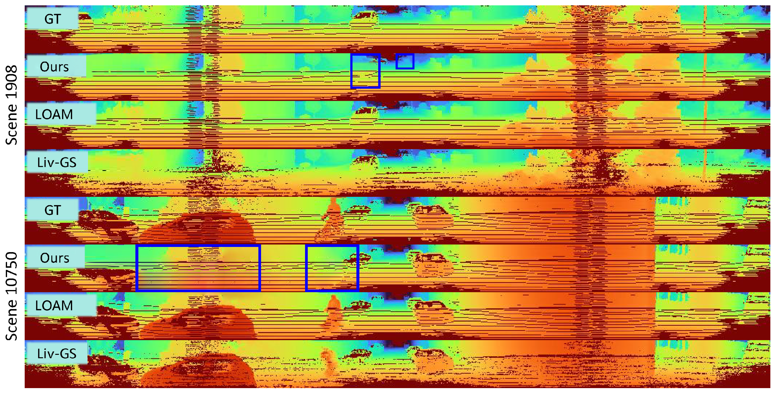
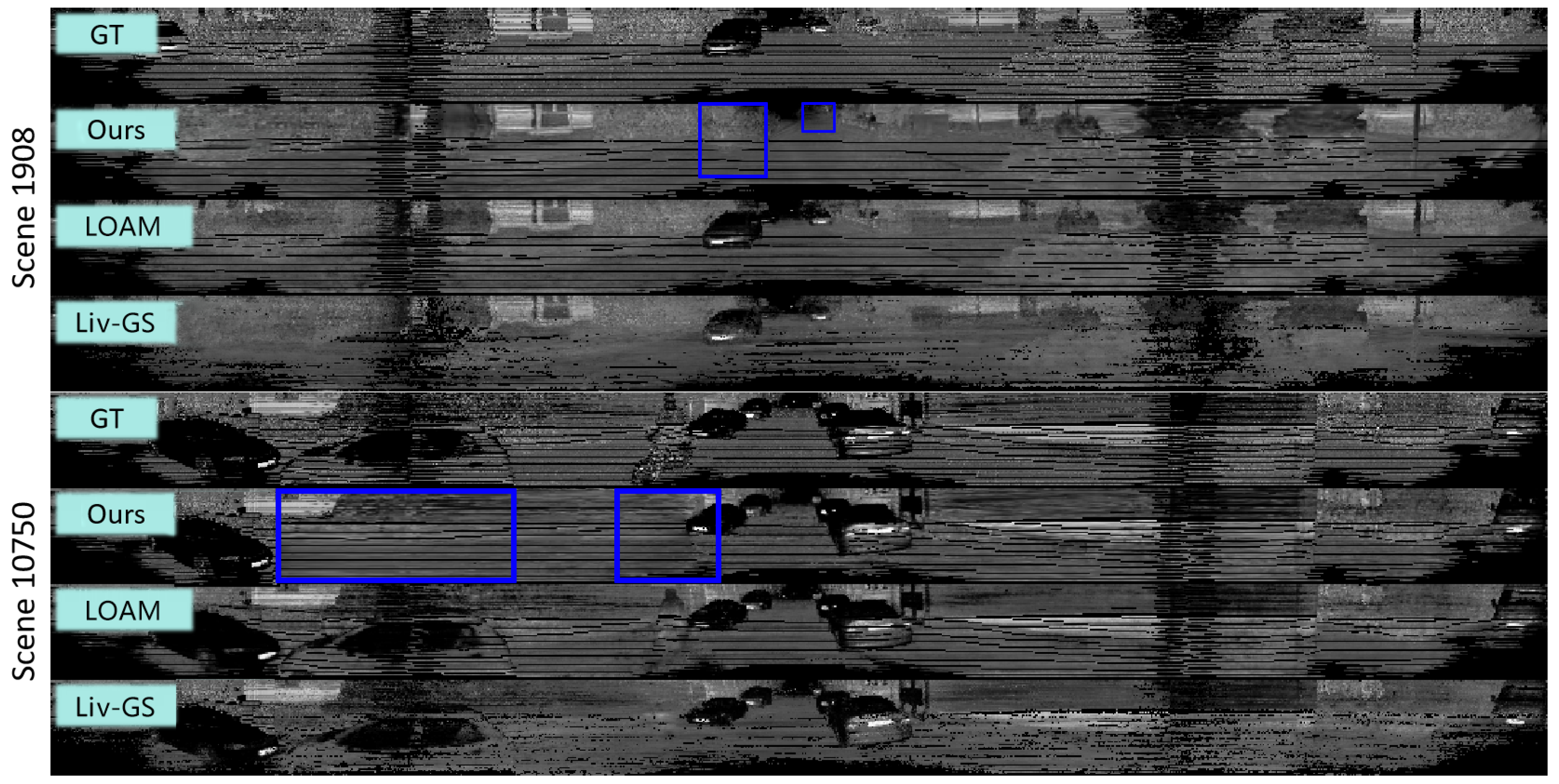
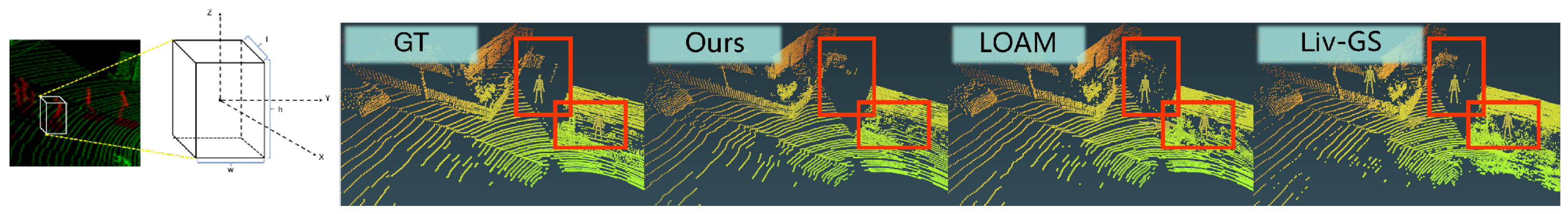
4.3. Mapping Results

For the qualitative mapping results, Figure 3 illustrates the differences between the proposed method, NeRF-LOAM, and LiV-GS in removing dynamic objects from outdoor street scenes in the KITTI dataset. The results show that the proposed method excels in reconstructing scenes with dynamic objects, offering a clear advantage in mitigating the interference caused by moving pedestrians and vehicles. In contrast, both NeRF-LOAM and LiV-GS demonstrate reduced performance when handling dynamic objects within street scenes. NeRF-LOAM particularly struggles with motion blur, while LiV-GS is capable of general scene reconstruction but fails to accurately remove the dynamic elements without distorting the static scene. On the other hand, our method is not only effective in removing dynamic objects but also restores the integrity of the street environment, maintaining a high level of detail and accuracy in the reconstruction. This is evident in the cleaner and more consistent representations of buildings, roads, and other static objects in the results, highlighting the superior dynamic object handling and scene fidelity of our approach.

Figure 4 presents the reconstruction results of the proposed method on industrial manufacturing scenarios from the ROI dataset. In complex industrial environments, our method excels at handling both static and dynamic objects. The proposed system effectively reconstructs the geometric structures of mechanical equipment and other industrial elements while maintaining accuracy, despite the presence of moving components such as robotic arms, forklifts, and human operators. Notably, our method maintains high-quality reconstructions even in highly cluttered environments with large machinery objects and varying levels of occlusion, which can often be problematic for conventional SLAM approaches. This adaptability to dynamic objects coupled with precise 3D reconstruction makes our approach particularly suitable for applications where robust and reliable scene reconstruction is essential for system operation, including automated inspection, production line monitoring, and real-time tracking of equipment. Its ability to differentiate and suppress dynamic interference ensures that critical structures are accurately mapped, enabling improved operational efficiency and safety in industrial settings.

Figure 5 presents the reconstruction results of the proposed method on outdoor scenes from the ROI dataset. Our method demonstrates remarkable adaptability in complex outdoor environments, accurately reconstructing both geometric structures and texture details despite the presence of various environmental challenges. These challenges include lighting variations, vegetation occlusions, and irregular terrain, all of which can negatively impact other SLAM systems. Our method effectively mitigates these challenges, ensuring that both the structure and appearance of the environment are captured with high fidelity. Notably, the system handles dynamic objects such as pedestrians and vehicles with remarkable accuracy. This ability to maintain high reconstruction accuracy even in the presence of dynamic elements is critical for applications such as outdoor navigation, environmental modeling, and autonomous driving technologies. The resilience of our method to dynamic interference ensures that it can be reliably used in real-world outdoor environments where unpredictable object movement is a frequent occurrence.

For the quantitative mapping results, we compared the proposed method with LDAR-NeRF [31], SHINE [32], NeRF-LOAM, and LiV-GS using the MaiCity and Newer College datasets.

Table 1. Mapping results on the MaiCity dataset [28]. Where lower values are better, and bold represents the best value.

Method	Completion ↓	Accuracy ↓	Chamfer-L1 Distance ↓	F-Score ↑
LDAR-NeRF	5.71	3.81	4.84	90.16
SHINE	4.35	4.08	4.26	89.94
NeRF-LOAM	4.16	3.29	3.68	93.51
LiV-GS	3.09	2.58	2.87	94.52
Ours	2.67	2.21	2.35	96.17

and

Table 2. Mapping results on the Newer College dataset [22]. Where lower values are better, and bold represents the best value.

Method	Completion ↓	Accuracy ↓	Chamfer-L1 Distance ↓	F-Score ↑
LDAR-NeRF	13.76	10.32	12.68	85.26
SHINE	14.39	8.57	11.45	90.43
NeRF-LOAM	16.01	6.95	10.94	91.85
LiV-GS	12.84	6.17	9.86	93.27
Ours	10.05	5.54	8.09	95.48

present the comparative results on these datasets, with the highest values for each metric highlighted in bold. The experimental results demonstrate that the proposed method consistently outperforms existing state-of-the-art approaches, especially in dynamic and complex environments. Our method shows significant improvements over the baseline systems in terms of accuracy, completeness, and F-score, which is especially evident in dynamic scenes. These results validate the effectiveness of our dynamic object removal strategy and multi-sensor fusion, as our method significantly reduces errors caused by moving objects, leading to more accurate and robust scene reconstructions. Furthermore, our method exhibits superior performance in terms of scene texture details, where the rendering quality and depth estimation are visibly better compared to other approaches.

We also compared our method with others in terms of rendered depth and radar point cloud reconstruction results, with the results shown in Figure 6 and Figure 7. The color map at the top of each figure represents the rendered depth map, while the grayscale map at the bottom shows the radar point cloud. Our method clearly outperforms the others in handling dynamic interference, particularly in its ability to accurately remove moving humans from radar images, thereby effectively eliminating their impact on the rendered depth. The removal of dynamic objects is consistent across both the tracking and rendering aspects. By removing the corresponding dynamic points in the radar point cloud results, our system achieves a more precise representation of the static scene, which is crucial for reliable SLAM operations in environments with moving objects. The ability to remove dynamic objects from both depth and point cloud data without compromising the integrity of the static scene represents a significant advancement over existing techniques, and ensures that the system can perform robustly even in challenging dynamic environments.

Overall, the results demonstrate that our approach offers substantial improvements over existing SLAM methods, particularly in terms of handling dynamic environments; the ability to remove dynamic objects with high accuracy while maintaining detailed and consistent reconstructions of static elements positions our system as a powerful tool for a wide range of applications, from autonomous navigation to industrial robotics.

The superior performance of our proposed method in highly dynamic scenes can be attributed to its innovative integration of LiDAR tracking, 3D point cloud segmentation, and 3DGS rendering, along with our introduction of a sliding window strategy to mitigate the impact of dynamic artifacts. Furthermore, use of the curling loss effectively addresses dynamic objects, enhancing both the accuracy and robustness of dense mapping. In contrast, other methods exhibit suboptimal performance in dynamic scenes, often struggling with reduced mapping accuracy due to interference caused by dynamic objects and artifacts.

4.4. Tracking Results

We conducted comprehensive comparative experiments between the proposed method, NeRF-LOAM, and LiV-GS across four distinct datasets to evaluate tracking performance. The results are summarized in

Table 3. Tracking results on the Newer College dataset. Where bold represents the best value.

Method	MaiCity	Newer College	KITTI	ROI-IND	ROI-OD
NeRF-LOAM	0.19	0.14	9.17	0.53	0.84
LiV-GS	0.08	0.08	8.21	0.41	0.65
Ours	0.06	0.01	6.57	0.19	0.32

, where the highest values for each metric are highlighted in bold. These experiments demonstrate that our method consistently outperforms both NeRF-LOAM and LiV-GS in terms of pose estimation accuracy and robustness, particularly in dynamic and complex environments.

First, our method exhibits significant improvements in pose estimation accuracy compared to NeRF-LOAM and LiV-GS on the KITTI dataset. The KITTI dataset is known for its challenging urban street scenes with moving pedestrians, vehicles, and complex building structures. The results on this dataset highlightsthe strength of our approach in handling dynamic interference. While NeRF-LOAM and LiV-GS show performance degradation when dynamic objects such as moving vehicles and pedestrians are present, our method effectively suppresses the influence of dynamic interference through a hybrid dynamic object removal strategy, allowing it to maintain accurate pose estimates even in environments with high dynamic complexity.

On the custom ROI dataset, which consists of both outdoor (ROI-OD) and industrial manufacturing (ROI-IND) scenarios, our method demonstrates significant versatility. In outdoor environments (ROI-OD), which often involve challenging conditions such as varying lighting, weather changes, and occlusions from trees or buildings, our method shows superior tracking accuracy. Its ability to adapt to these variations is highlighted by its lower pose estimation error of 0.32 compared to NeRF-LOAM’s 0.84 and LiV-GS’s 0.65. This underscores the robustness of our system in outdoor navigation tasks, where environmental dynamics and changing conditions are common.

Tracking accuracy in industrial manufacturing environments (ROI-IND) is particularly challenging, as dynamic objects such as robotic arms, conveyor belts, and workers frequently move around. Despite these complexities, our system manages to maintain an impressive pose estimation error of 0.19. This performance is significantly better than that of NeRF-LOAM and LiV-GS, which show pose estimation errors of 0.53 and 0.41, respectively. These results illustrate the strength of our method for applications where precise tracking is essential for maintaining workflow continuity and safety, such as automated inspection and production line monitoring.

The results shown in Table 3 clearly demonstrate that our method offers significant improvements in pose estimation accuracy across all datasets. Our system achieves the lowest errors on both the MaiCity and Newer College datasets, confirming its generalization capability across different environments. The consistency of our tracking algorithm’s performance across various datasets ranging from urban streets to industrial environments underscores its robustness and versatility in diverse real-world scenarios.

The results further demonstrate the effectiveness of our dynamic interference removal strategy. In contrast to other methods, which struggle with dynamic humans and produce scanning point clouds that include moving objects, our approach employs a hybrid segmentation strategy based on both visual uncertainty and 3D object detection. This segmentation strategy allows us to distinguish dynamic objects from the static scene more accurately and remove them from the point cloud. As shown in Figure 8, the point cloud produced by our method is cleaner, with noise points from dynamic objects effectively removed. This leads to more precise tracking and pose estimation, as dynamic interference is suppressed without affecting the underlying static structures. The effectiveness of our dynamic object removal strategy is particularly critical in applications where moving objects could otherwise disrupt the accuracy of tracking, such as in autonomous driving or industrial robotics contexts.

Our method’s performance in dynamic environments highlights its superior ability to suppress interference from dynamic objects, which is one of the key challenges in SLAM. By leveraging both segmentation and sensor fusion techniques, our approach can remove dynamic interference from both LiDAR and visual data, ensuring that the pose estimation remains accurate even in the presence of moving objects. The results on all datasets demonstrate that the combination of these techniques provides a robust solution to the dynamic object problem, making our system highly applicable to real-world dynamic environments.

Overall, our tracking results show that the proposed method not only achieves superior performance compared to state-of-the-art techniques but also demonstrates significant versatility and robustness in handling dynamic and complex environments. This positions our method as a reliable solution for real-time tracking and pose estimation in challenging dynamic settings where other methods can struggle to maintain accuracy.

4.5. Ablation Study

To further validate the effectiveness of the proposed method, we conducted extensive ablation experiments using the MaiCity dataset. The following tables present the results with different experimental settings, including variations in the sliding window length and rendering loss functions.

Table 4. Results of ablation study on the MaiCity dataset with different sliding window lengths. Where lower values are better, and bold represents the best value.

Window Length	Completion ↓	Accuracy ↓	Chamfer-L1 Distance ↓	F-Score ↑
No Window	3.86	3.18	3.52	91.34
$w=10$	3.25	2.79	2.71	94.12
$w=20$	2.67	2.21	2.35	96.17
$w=30$	3.49	2.54	2.86	93.58
$w=40$	3.74	2.99	3.67	90.81

shows the quantitative evaluation results with varying sliding window lengths. The sliding window strategy plays a crucial role in improving the performance of the system. The highest values for each metric are highlighted in bold. The results indicate that omitting the sliding window strategy (No Window) leads to a significant performance drop across all metrics. The system achieves the best performance with a window length of $w=20$, as evidenced by the lowest completion, accuracy, and Chamfer-L1 distance coupled with the highest F-score. However, the performance starts to degrade as w exceeds this optimal value, especially in terms of completion and accuracy.

The degradation in performance for larger window lengths, particularly $w=40$, can be attributed to increased computational complexity, reduced sensitivity to local scene variations, and accumulated dynamic interference. Larger window sizes require more computational resources, which may lead to delays and reduced real-time performance. Additionally, a larger window may fail to capture rapid changes in local scenes, resulting in less effective dynamic object removal. Furthermore, dynamic objects may persist across multiple frames in larger windows, leading to artifacts in the static scene reconstruction. These factors collectively explain why $w=40$ exhibits the worst performance among the tested window lengths.

From these results, it is clear that the window length plays a critical role in fine-tuning the system’s performance. As w becomes larger than 20, our proposed method becomes less sensitive to local scene variations, resulting in poorer performance.

Table 5. Results of ablation study on the MaiCity dataset with different rendering losses. Where lower values are better, and bold represents the best value.

Rendering Losses	Completion ↓	Accuracy ↓	Chamfer-L1 Distance ↓	F-Score ↑
w/o ${\mathcal{L}}_c$	4.27	3.45	3.79	92.36
w/o ${\mathcal{L}}_d$	3.54	2.87	3.05	94.28
w/o ${\mathcal{L}}_{edge}$	5.13	3.96	4.76	90.89
FULL	2.67	2.21	2.35	96.17

presents the ablation study results with different rendering losses. We evaluated the impact of each individual loss function—completion loss ${\mathcal{L}}_c$, depth loss ${\mathcal{L}}_d$, and edge loss ${\mathcal{L}}_{edge}$—on overall system performance. As seen in the results, omitting any one of these losses reduces the overall accuracy and completeness of the reconstruction.

For example, when the completion loss ${\mathcal{L}}_c$ is excluded, the system experiences a slight degradation in performance, with higher completion and Chamfer-L1 distance values. Exclusion of the depth loss ${\mathcal{L}}_d$ also causes a noticeable drop in accuracy, indicating its importance for depth-aware optimization. Finally, removing the edge loss ${\mathcal{L}}_{edge}$ leads to the largest performance drop in terms of both completion and F-score, as this loss function significantly contributes to preserving structural details in the reconstruction.

These findings strongly suggest that all three loss functions play an essential role in optimizing different aspects of the system, including geometric fidelity, accuracy, and feature preservation.

5. Conclusions

In this paper, we have proposed a dynamic scene-oriented LiDAR fusion SLAM framework based on 3D Gaussian Splatting. By integrating LiDAR point clouds, 3D semantic segmentation, and 3DGS rendering, our method addresses dynamic interference and large-scale scene reconstruction challenges. Through its use of a sliding window strategy, dynamic point cloud occupancy management, and novel loss functions, our system shows significantly improved accuracy and robustness in dynamic environments.

Experiments on public and custom datasets show that our system outperforms state-of-the-art methods, particularly in dynamic outdoor and industrial environments. Our approach effectively reconstructs static backgrounds, removes dynamic artifacts, and maintains scene fidelity. Its ability to handle dynamic objects while preserving scene features demonstrates potential for real-world applications such as autonomous navigation and intelligent manufacturing.

While the proposed system achieves optimal performance with a window length of $w=20$, further improvements could be made for other window lengths. For $w=10$, the system could benefit from enhanced sensitivity to local scene variations, potentially through adaptive window sizing or multiscale analysis. For larger window lengths such as $w=30$ and $w=40$, reducing computational complexity and improving dynamic object removal efficiency are critical. Techniques such as parallel processing, optimized data structures, and advanced dynamic object detection algorithms could be explored to address these challenges.

Despite these advancements, there are a number of limitations. The computational complexity of the proposed system can be an issue when processing large-scale or highly dense environments. While it performs well in many cases, delays can occur with large datasets or dense scenes, potentially affecting real-time performance. Additionally, reliance on accurate dynamic object detection and segmentation may cause issues in unstructured or ambiguous environments, where segmentation accuracy may degrade and transient objects may still introduce errors.

Future work will focus on improving computational efficiency, developing optimized segmentation models, and enhancing adaptability to challenging environments. We also plan to explore additional sensor modalities such as radar in order to increase robustness in conditions such as low visibility or extreme weather.

References

1. Mildenhall, B.; Srinivasan, P.P.; Tancik, M.; Barron, J.T.; Ramamoorthi, R.; Ng, R. Nerf: Representing scenes as neural radiance fields for view synthesis. Commun. ACM 2021, 65, 99–106. [Google Scholar] [CrossRef]
2. Rosinol, A.; Leonard, J.J.; Carlone, L. Nerf-slam: Real-time dense monocular slam with neural radiance fields. In Proceedings of the 2023 IEEE/RSJ International Conference on Intelligent Robots and Systems (IROS), Detroit, MI, USA, 1–5 October 2023; pp. 3437–3444. [Google Scholar]
3. Li, M.; Guo, Z.; Deng, T.; Zhou, Y.; Ren, Y.; Wang, H. DDN-SLAM: Real Time Dense Dynamic Neural Implicit SLAM. IEEE Robot. Autom. Lett. 2025, 1–8. [Google Scholar] [CrossRef]
4. Chung, C.M.; Tseng, Y.C.; Hsu, Y.C.; Shi, X.Q.; Hua, Y.H.; Yeh, J.F.; Chen, W.C.; Chen, Y.T.; Hsu, W.H. Orbeez-slam: A real-time monocular visual slam with orb features and nerf-realized mapping. In Proceedings of the 2023 IEEE International Conference on Robotics and Automation (ICRA), London, UK, 29 May–2 June 2023; pp. 9400–9406. [Google Scholar]
5. Yang, F.; Wang, Y.; Tan, L.; Li, M.; Shan, H.; Liao, P. DNIV-SLAM: Neural Implicit Visual SLAM in Dynamic Environments. In Proceedings of the Chinese Conference on Pattern Recognition and Computer Vision (PRCV), Urumqi, China, 18–20 October 2024; pp. 33–47. [Google Scholar]
6. Naumann, J.; Xu, B.; Leutenegger, S.; Zuo, X. Nerf-vo: Real-time sparse visual odometry with neural radiance fields. IEEE Robot. Autom. Lett. 2024, 9, 7278–7285. [Google Scholar] [CrossRef]
7. Lu, L.; Zhang, Y.; Zhou, P.; Qi, J.; Pan, Y.; Fu, C.; Pan, J. Semantics-Aware Receding Horizon Planner for Object-Centric Active Mapping. IEEE Robot. Autom. Lett. 2024, 9, 3838–3845. [Google Scholar] [CrossRef]
8. Yan, C.; Qu, D.; Xu, D.; Zhao, B.; Wang, Z.; Wang, D.; Li, X. Gs-slam: Dense visual slam with 3D gaussian splatting. In Proceedings of the IEEE/CVF Conference on Computer Vision and Pattern Recognition, Seattle, WA, USA, 16–22 June 2024; pp. 19595–19604. [Google Scholar]
9. Zhai, H.; Huang, G.; Hu, Q.; Li, G.; Bao, H.; Zhang, G. Nis-slam: Neural implicit semantic rgb-d slam for 3D consistent scene understanding. IEEE Trans. Vis. Comput. Graph. 2024, 30, 7129–7139. [Google Scholar] [CrossRef] [PubMed]
10. Matsuki, H.; Murai, R.; Kelly, P.H.J.; Davison, A.J. Gaussian Splatting SLAM. In Proceedings of the IEEE/CVF Conference on Computer Vision and Pattern Recognition, Seattle, WA, USA, 16–22 June 2024. [Google Scholar]
11. Li, M.; Liu, S.; Zhou, H.; Zhu, G.; Cheng, N.; Deng, T.; Wang, H. Sgs-slam: Semantic gaussian splatting for neural dense slam. In Proceedings of the European Conference on Computer Vision, Milan, Italy, 29 September–4 October 2024; pp. 163–179. [Google Scholar]
12. Keetha, N.; Karhade, J.; Jatavallabhula, K.M.; Yang, G.; Scherer, S.; Ramanan, D.; Luiten, J. SplaTAM: Splat Track & Map 3D Gaussians for Dense RGB-D SLAM. In Proceedings of the IEEE/CVF Conference on Computer Vision and Pattern Recognition, Seattle, WA, USA, 16–22 June 2024; pp. 21357–21366. [Google Scholar]
13. Deng, J.; Wu, Q.; Chen, X.; Xia, S.; Sun, Z.; Liu, G.; Yu, W.; Pei, L. Nerf-loam: Neural implicit representation for large-scale incremental lidar odometry and mapping. In Proceedings of the IEEE/CVF International Conference on Computer Vision, Paris, France, 1–6 October 2023; pp. 8218–8227. [Google Scholar]
14. Isaacson, S.; Kung, P.C.; Ramanagopal, M.; Vasudevan, R.; Skinner, K.A. Loner: Lidar only neural representations for real-time slam. IEEE Robot. Autom. Lett. 2023, 8, 8042–8049. [Google Scholar] [CrossRef]
15. Pan, Y.; Zhong, X.; Wiesmann, L.; Posewsky, T.; Behley, J.; Stachniss, C. PIN-SLAM: LiDAR SLAM using a point-based implicit neural representation for achieving global map consistency. IEEE Trans. Robot. 2024, 40, 4045–4064. [Google Scholar] [CrossRef]
16. Carlson, A.; Ramanagopal, M.S.; Tseng, N.; Johnson-Roberson, M.; Vasudevan, R.; Skinner, K.A. Cloner: Camera-lidar fusion for occupancy grid-aided neural representations. IEEE Robot. Autom. Lett. 2023, 8, 2812–2819. [Google Scholar] [CrossRef]
17. Li, Y.; Yu, A.W.; Meng, T.; Caine, B.; Ngiam, J.; Peng, D.; Shen, J.; Lu, Y.; Zhou, D.; Le, Q.V.; et al. Deepfusion: Lidar-camera deep fusion for multi-modal 3D object detection. In Proceedings of the IEEE/CVF Conference on Computer Vision and Pattern Recognition, New Orleans, LA, USA, 18–24 June 2022; pp. 17182–17191. [Google Scholar]
18. Lang, X.; Li, L.; Zhang, H.; Xiong, F.; Xu, M.; Liu, Y.; Zuo, X.; Lv, J. Gaussian-LIC: Photo-realistic LiDAR-Inertial-Camera SLAM with 3D Gaussian Splatting. arXiv 2024, arXiv:2404.06926. [Google Scholar]
19. Zhou, X.; Lin, Z.; Shan, X.; Wang, Y.; Sun, D.; Yang, M.H. Drivinggaussian: Composite gaussian splatting for surrounding dynamic autonomous driving scenes. In Proceedings of the IEEE/CVF Conference on Computer Vision and Pattern Recognition, Seattle, WA, USA, 16–22 June 2024; pp. 21634–21643. [Google Scholar]
20. Cui, J.; Cao, J.; Zhao, F.; He, Z.; Chen, Y.; Zhong, Y.; Xu, L.; Shi, Y.; Zhang, Y.; Yu, J. LetsGo: Large-scale garage modeling and rendering via LiDAR-assisted gaussian primitives. ACM Trans. Graph. (TOG) 2024, 43, 1–18. [Google Scholar] [CrossRef]
21. Hong, S.; He, J.; Zheng, X.; Zheng, C.; Shen, S. Liv-gaussmap: Lidar-inertial-visual fusion for real-time 3D radiance field map rendering. IEEE Robot. Autom. Lett. 2024, 9, 9765–9772. [Google Scholar] [CrossRef]
22. Liang, T.; Xie, H.; Yu, K.; Xia, Z.; Lin, Z.; Wang, Y.; Tang, T.; Wang, B.; Tang, Z. Bevfusion: A simple and robust lidar-camera fusion framework. Adv. Neural Inf. Process. Syst. 2022, 35, 10421–10434. [Google Scholar]
23. Lee, J.C.; Rho, D.; Sun, X.; Ko, J.H.; Park, E. Compact 3D gaussian representation for radiance field. In Proceedings of the IEEE/CVF Conference on Computer Vision and Pattern Recognition, Seattle, WA, USA, 16–22 June 2024; pp. 21719–21728. [Google Scholar]
24. Xiao, R.; Liu, W.; Chen, Y.; Hu, L. LiV-GS: LiDAR-Vision Integration for 3D Gaussian Splatting SLAM in Outdoor Environments. IEEE Robot. Autom. Lett. 2024, 10, 421–428. [Google Scholar] [CrossRef]
25. Sandström, E.; Li, Y.; Van Gool, L.; Oswald, M.R. Point-slam: Dense neural point cloud-based slam. In Proceedings of the IEEE/CVF International Conference on Computer Vision, Paris, France, 1–6 October 2023; pp. 18433–18444. [Google Scholar]
26. Huber, P.J. Robust estimation of a location parameter. In Breakthroughs in Statistics: Methodology and Distribution; Springer: Berlin/Heidelberg, Germany, 1992; pp. 492–518. [Google Scholar]
27. Geiger, A.; Lenz, P.; Urtasun, R. Are we ready for autonomous driving? The kitti vision benchmark suite. In Proceedings of the 2012 IEEE Conference on Computer Vision and Pattern Recognition, Providence, RI, USA, 16–21 June 2012; pp. 3354–3361. [Google Scholar]
28. Vizzo, I.; Chen, X.; Chebrolu, N.; Behley, J.; Stachniss, C. Poisson surface reconstruction for LiDAR odometry and mapping. In Proceedings of the 2021 IEEE International Conference on Robotics and Automation (ICRA), Xi’an, China, 30 May–5 June 2021; pp. 5624–5630. [Google Scholar]
29. Ramezani, M.; Wang, Y.; Camurri, M.; Wisth, D.; Mattamala, M.; Fallon, M. The newer college dataset: Handheld lidar, inertial and vision with ground truth. In Proceedings of the 2020 IEEE/RSJ International Conference on Intelligent Robots and Systems (IROS), Las Vegas, NV, USA, 24 October 2020–24 January 2021; pp. 4353–4360. [Google Scholar]
30. Hu, H.N.; Yang, Y.H.; Fischer, T.; Darrell, T.; Yu, F.; Sun, M. Monocular quasi-dense 3D object tracking. IEEE Trans. Pattern Anal. Mach. Intell. 2022, 45, 1992–2008. [Google Scholar] [CrossRef] [PubMed]
31. Tao, T.; Gao, L.; Wang, G.; Lao, Y.; Chen, P.; Zhao, H.; Hao, D.; Liang, X.; Salzmann, M.; Yu, K. LiDAR-NeRF: Novel lidar view synthesis via neural radiance fields. In Proceedings of the 32nd ACM International Conference on Multimedia, Melbourne, Australia, 28 October–1 November 2024; pp. 390–398. [Google Scholar]
32. Zhong, X.; Pan, Y.; Behley, J.; Stachniss, C. Shine-mapping: Large-scale 3D mapping using sparse hierarchical implicit neural representations. In Proceedings of the 2023 IEEE International Conference on Robotics and Automation (ICRA), London, UK, 29 May–2 June 2023; pp. 8371–8377. [Google Scholar]
Figure 1. Overall framework of our system. The figure illustrates the architecture of the proposed 3DGS-based SLAM system integrating LiDAR and vision data for dynamic scene tracking and reconstruction. The input (left) shows raw sensor data, while the output (right) demonstrates the reconstructed static scene with dynamic objects removed.
Applsci 15 04190 g001
Figure 2. Comparison of mapping results on the KITTI dataset.
Applsci 15 04190 g002
Figure 3. Comparison of mapping results in the industrial scenarios of the ROI dataset (ROI-IND).
Applsci 15 04190 g003
Figure 4. Comparison of mapping results in the outdoor scenarios of the ROI dataset (ROI-OD).
Applsci 15 04190 g004
Figure 5. Depth rendering result after removing dynamic objects.
Applsci 15 04190 g005
Figure 6. LiDAR point cloud result after removing dynamic objects.
Applsci 15 04190 g006
Figure 7. Demonstration of the 3D bounding box setup and the effect of removing laser point clouds. Our method effectively addresses dynamic interference compared to other methods, resulting in a cleaner point cloud with noise points removed.
Applsci 15 04190 g007
Figure 8. Our method effectively removes dynamic objects such as pedestrians, vehicles from the LiDAR point cloud, achieving cleaner static scene reconstruction; in contrast, NeRF-LOAM fails to eliminate dynamic interference, resulting in artifacts and errors.
Applsci 15 04190 g008