Hybrid Compensation Method for Non-Uniform Creep Difference and Hysteresis Nonlinearity of Piezoelectric-Actuated Machine Tools Under S-Shaped Curve Trajectory

Abstract

Piezoelectric-actuated machine tools (PAMTs) exhibit nanoscale motion capabilities, with their S-shaped curve trajectory further enabling smooth path execution and reduced terminal pulse. However, the speed changes inherent in multi-order trajectories introduce an additional non-uniform creep difference (NCD), which differs significantly from conventional hysteresis effects. Traditional models are inadequate for addressing this mixed shape nonlinearity. To overcome this limitation, this paper proposes a hybrid compensation method for the S-shaped curve trajectory of piezoelectric-actuated machine tools. The general deformation law is first established through a comprehensive mechanism analysis. The NCD and hysteresis, induced by speed changes and inherent properties, are decoupled and addressed using a pre-known phenomenon model and a clockwise operator model, respectively. Finally, a hybrid feedforward control strategy is developed to integrate these models for effective compensation. Experimental results demonstrate that the hybrid compensation method achieves a maximum relative error of 5.48% and a maximum mean square error of 0.28%, effectively mitigating the dual nonlinear factors arising from the piezoelectric-actuated machine tool’s trajectory in feedforward control.

1. Introduction

Piezoelectric-actuated machine tools (PAMTs) use piezoelectric actuators as their core components. Their high resolution, fast response, high stiffness, and micro deformation characteristics enable precise nanoscale displacement control [1,2,3], making them a key technological carrier in the field of ultra-precision machining. In practical machining [4,5], the tool must balance the requirements of “flexible feed” and “flexible retreat” during the reciprocating high-speed movement [6,7]. It is necessary to avoid rigid impact damage to the workpiece surface at the moment of contact and maintain machining efficiency through high-frequency micro motion. S-shaped curvetrajectory planning effectively solves the inertia impact problem caused by sudden acceleration changes in traditional trapezoidal trajectories through continuous and smooth velocity and acceleration curve design. It not only reduces the vibration of the machining, but also shortens the idle travel time through dynamic optimization of the velocity curves [8,9]. This characteristic not only fully utilizes the nanoscale dynamic adjustment capability of piezoelectric actuators but also transforms their high-frequency response advantages into stable high-frequency micro-cutting functions, thereby achieving a synergistic improvement in surface quality and processing efficiency in ultra-precision machining.

The piezoelectric actuator is affected by many factors, such as the polarization process, the doping preparation, the strong external electric field or the high stress [10,11]. Nonlinear effects, such as hysteresis, creep, and rate-dependent dynamics, directly cause deviations between the expected S-shaped curvetrajectory and the actual output [12,13]. In addition, because the S-shaped trajectory driving voltage couples multiple common motion characteristics, the speed changes inherent in such multistage trajectories introduce additional non-uniform creep differences (NCD), which not only reduce tracking accuracy, but also cause unnecessary oscillations that affect surface smoothness and tool life. Therefore, compensating the non-linearity of the hysteretic coupling NCD can effectively improve the accuracy of trajectory tracking and the output performance of PAMTs. For nonlinear compensation of piezoelectric actuators, most studies utilize traditional phenomenological models to describe hysteresis more accurately, and design inverse model controllers to compensate for nonlinearity [14,15]. For example, Ayad G et al. employ an improved Preisach hysteresic model and two-degree -of-freedom H-Infinity robust control to precisely control the motion of piezoelectric actuators. The results obtained by using this control strategy show that the lag modeling accuracy and tracking performance are significantly improved, and the mean root mean square error (RMSE) is 0.0107 µm and 0.0212 µm, respectively [16]. Xu et al. investigated an improved Prandtl Ishlinskii (PI) model that utilizes a one-sided dead zone operator to overcome the proposed hysteresis asymmetry of the actuator. Comparing the improved PI model with the traditional PI model, the BoucWen model, and experimental data, the maximum relative error is only 5.70%, and the model fitting accuracy is greater than 0.99 [17]. Liu et al. proposed a hyperplane probabilistic c-regression model (HPCRM) algorithm and established its hysterically nonlinear TS fuzzy model [18]. However, these studies only compensate for the single nonlinear feature of hysteresis, and do not take into account the coupled nonlinearity of factors such as creep.

On the other hand, the creep behavior of piezoelectric actuators is usually described by combining hysteresis models, which are mainly divided into logarithmic creep models, linear time-invariant (LTI) creep models, and fractional-order models [19,20,21]. The logarithmic creep model and LTI creep model can be used in parallel or in series with the hysteresis model to comprehensively describe the hysteresis and creep phenomena of piezoelectric actuators. This combination allows hysteresis and creep models to operate independently with low coupling. For example, Jung et al. proposed the concept of “voltage creep”, assuming that constant displacement may cause input voltage creep, and developed a logarithmic creep model based on this to compensate for the nonlinear behavior of piezoelectric actuators [22]. Nie et al. further designed a logarithmic creep controller combined with a PI model to achieve open-loop control of piezoelectric actuators [23]. Changhai et al. proposed hysteresis and logarithmic creep models, and used inverse feedforward control to simultaneously compensate for the hysteresis and creep of piezoelectric actuators [24].

In addition, there are studies combining the creep model with the hysteresis model. Krejci et al. extended an operator-based hysteresis model and provided a physical structure diagram including hysteresis and creep [25]. Kuhnenet et al. developed a feedforward controller based on the LTI creep model and hysteresis operator to compensate for the hysteresis and creep of piezoelectric actuators [26]. Mokaberi et al. modeled the nonlinear effects of hysteresis and creep based on the superposition of basic operators, describing the creep operator as a linear first-order system [27]. Yang et al. combined the PI model and LTI model to propose a compensator that integrates an adaptive controller and an online approximator to compensate for the creep and hysteresis of piezoelectric actuators [28]. Through the comparative analysis of existing research methods in

Table 1. Comparison of existing methods.

Nonlinear Factors	Solution	Advantage	Limitation
Hysteresis	Improved Preisach hysteresis model [16] Improved Prandtl–Ishlinskii (PI) model [17] TS fuzzy model [18]	They address the asymmetric features and dead zone issues in hysteresis characteristics.	Only consider the nonlinear effect of hysteresis on piezoelectric actuators, without taking into account creep characteristics
Creep	Logarithmic creep models [19] Linear time-invariant (LTI) creep models [20] Fractional-order models [21]	The models are simple and easy to implement, suitable for open-loop control.	Poor dynamic adaptability; reliance on empirical parameters
Hysteresis + Creep	A feedforward controller based on the LTI creep model and hysteresis operator [22] The nonlinear effects of hysteresis and creep [23] A compensator combining the PI model and LTI model [24]	They provide a more comprehensive description of nonlinearity (such as operator superposition, adaptive combination).	Complex calculations and insufficient real-time performance; most of them did not consider strong coupling effects

, it can be seen that the existing research mainly focuses on hysteretic characteristics and nonlinearity caused by static creep, while ignoring the nonlinear influence caused by NCD. The traditional model is not enough to solve the mixed-shape nonlinear problem.

Based on the above facts, in order to solve the mixed nonlinearity of piezoelectric actuators in multi-stage trajectories, the coupling mechanism between the hysteresis nonlinearity of piezoelectric actuators and NCDs in S-shaped curve trajectory is studied in this paper, and a hybrid feedforward control strategy is proposed to realize the preset trajectory shaping. The purpose is to separate NCD and hysteresis and to compensate for the coupling nonlinearity. The effectiveness of this strategy is verified by an experimental case study. This research helps to improve the applicability of S-shaped curve trajectory in piezoelectric drive systems and bridge the gap between theoretical motion planning and practical nonlinear control challenges.

The main innovations of this paper include the following: a method of NCD separation is proposed, a hybrid feedforward control strategy is designed, and the lag problem is solved by using the clockwise operator. This hybrid control strategy applies not only to the S-trajectory drive voltage in PAMTs, but also can be further extended to other multi-stage trajectories. In addition, this control idea can also be used for reference for other piezoelectric actuating equipment to adapt to its specific working conditions.

The main structure of this article is as follows: Section 2 introduces the typical structure of PAMTs, derives the general deformation law of piezoelectric actuators, and theoretically analyzes the complex nonlinearity of piezoelectric actuators under S-shaped trajectory driving voltage. Section 3 analyzes the mechanism of NCD, proposes an NCD separation method, and proposes a hybrid control strategy combining nonlinear compensation and trajectory shaping. Section 4 validates the proposed method through experiments. Section 5 provides a summary of the article.

2. Background and Driving Principles

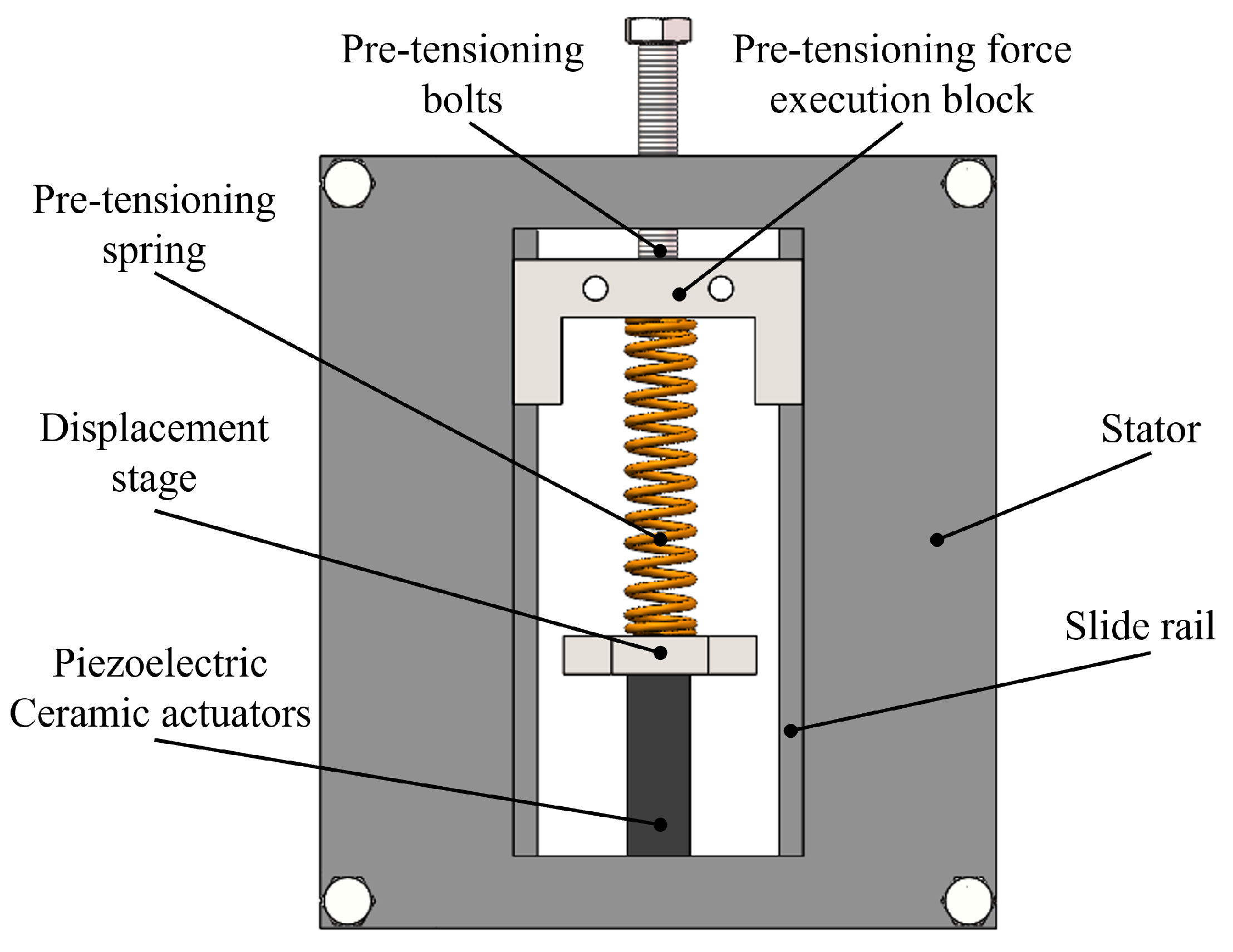
2.1. Structure of Typical PAMTs

Figure 1 provides a schematic diagram of a typical PAMT structure. The main components of PAMTs include the tool platform, planar flexible hinges, hinge fixation devices, piezoelectric actuator, piezoelectric actuator fixation devices, preload screws, and preload nuts. Among these, dual parallel flexible hinges are used to achieve high-precision motion transmission. The flexible hinges enable elastic deformation motion within the nanometer range while eliminating friction, ensuring efficient transmission of force and motion. Before machining, the required preload force can be applied to the piezoelectric actuator using the preload screws to optimize their performance. The vibration isolation platform is used to isolate external vibrations from affecting the tool holder, stabilizing the tool holder and ensuring machining accuracy. Since tensile and shear forces significantly impact the performance and lifespan of a piezoelectric actuator, the piezoelectric actuator cannot directly drive the cutting tool. Therefore, a guiding mechanism is designed to protect the piezoelectric actuator. The guiding mechanism must accurately transmit the displacement of the piezoelectric actuator to the tool under high-frequency motion while ensuring stability and precision. This structural design, through the combination of flexible hinges and guiding mechanisms, achieves efficient motion transmission between the piezoelectric actuator and the cutting tool while preventing damage to the piezoelectric actuator due to direct force application. This enhances the system’s reliability and machining accuracy.

The PAMT requires a micro-positioning stage with high precision, large stroke, and high stiffness. It typically employs a coarse and fine two-stage feed system, where constant-velocity motion ensures the best machining quality. Generally, a micro-positioning stage with a stroke range of 0 to 40 nm can meet the requirements of fine feed. The designed stage must have high stiffness to counteract machine tool vibrations and cutting forces during the machining process, ensuring machining accuracy and stability. The specific technical parameters of PAMTs are listed in

Table 2. Technical parameters of PAMT structure.

Technical Indicators	Numeric Value	Unit
Stiffness	24.5	µm/N
Maximum displacement	45 ± 1	µm
Displacement loss ratio	18.3% ± 0.6
Hinge minimum width d	1	mm
Hinge cutout radius R	2	mm
Span length L	22	mm
Spring recovery force	1344	N
Piezo minimum preload	968	N
Natural frequencies	858.8	Hz

.

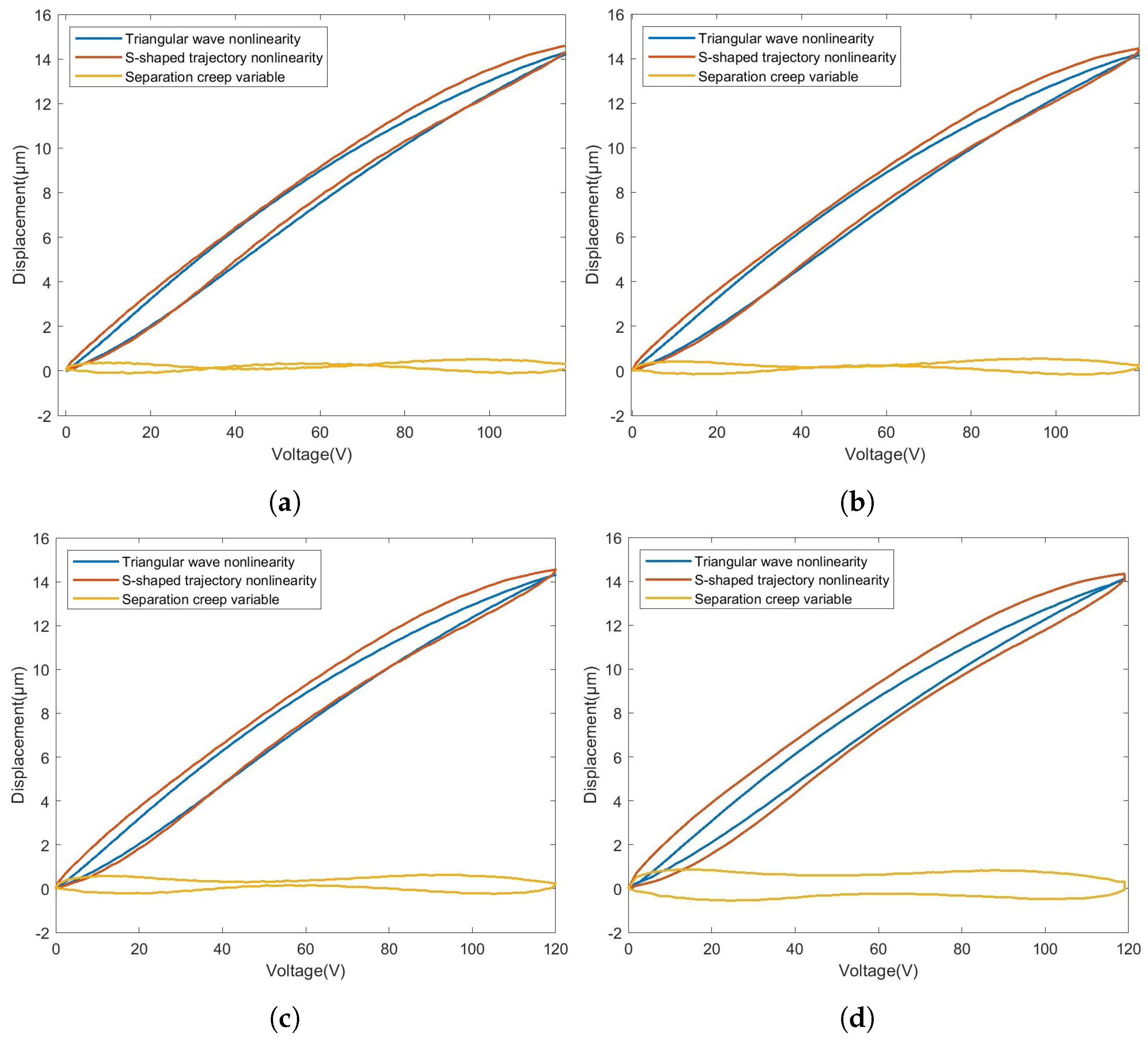
2.2. Analysis of Nonlinear Characteristics of Piezoelectric Actuators Under S-Shaped Trajectory Driving Voltage

The dynamic behavior of piezoelectric actuators is jointly influenced by their electrical properties, mechanical properties, and the coupling effects between them. The electrical behavior of piezoelectric actuators can be modeled as an equivalent parallel circuit, where R represents the leakage resistance of the material, reflecting the dissipation of internal charge, and C represents the equivalent capacitance of the material, reflecting its ability to store charge. In this equivalent circuit, the time constant $\tau =RC$ is referred to as the first-order relaxation time.

The dielectric response of piezoelectric actuators is determined by the internal electric dipole moments. When an external electric field is applied, the field drives the rearrangement of the internal electric dipole moments, resulting in polarization. Additionally, the rearrangement of electric dipole moments requires overcoming lattice barriers or internal molecular resistance, leading to a time delay in the polarization process. This time delay is determined by the material’s internal atomic structure and thermodynamic behavior, manifesting as a typical relaxation process. The dielectric relaxation behavior of piezoelectric ceramics can be described via the Debye model [29]. Its fundamental assumption is that the response of electric dipole moments follows a first-order relaxation process, satisfying the following dynamic equation:

$${\displaystyle \frac{dP}{dt}}+{\displaystyle \frac{P}{\tau }}={ϵ}_0{\displaystyle \frac{dE}{dt}}$$

(1)

where P is the polarization intensity; E is the applied electric field intensity; $\tau$ is the relaxation time; and ${ϵ}_0$ is the vacuum permittivity. By solving this equation, the complex dielectric constant of the material in the frequency domain is obtained:

$$\epsilon \left(\omega \right)={\epsilon }_{\infty }+{\displaystyle \frac{{\epsilon }_s-{\epsilon }_{\infty }}{1+{\left(\omega \tau \right)}^2}}(\mathrm{Real}\mathrm{part})$$

(2)

$${\epsilon }^{*}\left(\omega \right)={\epsilon }_{\infty }+{\displaystyle \frac{({\epsilon }_s-{\epsilon }_{\infty })\omega \tau }{1+{\left(\omega \tau \right)}^2}}(\mathrm{Imaginary}\mathrm{part})$$

(3)

where ${\epsilon }_{\infty }$ is the static dielectric constant at a high frequency; ${\epsilon }_s$ is the static dielectric constant at a low frequency; $\omega$ is the angular frequency; and $\tau$ is the relaxation time.

When $\omega \tau \ll 1$ (low frequency), the material has sufficient time to respond to the electric field, and the complex dielectric constant $\epsilon \approx {\epsilon }_s$. When $\omega \tau \gg 1$ (high frequency), the electric dipole moments cannot follow the changes in the electric field, and the complex dielectric constant $\epsilon \approx {\epsilon }_{\infty }$. This phenomenon can be explained by the electromechanical dynamic coupling theory.

The mechanical dynamic response of piezoelectric actuators can be characterized by the electromechanical coupling constitutive equations—specifically, the following:

$$S=sT+d^{T}E$$

(4)

$$D=dT+\epsilon E$$

(5)

where S is the strain; T is the stress; E is the applied electric field intensity; D is the electric displacement; s is the compliance matrix (elastic compliance under a constant electric field); d is the piezoelectric constant matrix; $d^T$ is the transpose of the piezoelectric constant matrix; and $\epsilon$ is the dielectric constant matrix (dielectric constant under constant stress).

By introducing a frequency-dependent dielectric constant model, as shown in Equations (6) and (7), the suppression effect of dielectric relaxation on the charge quantity under variable frequency conditions can be revealed. Specifically, the charge quantity $Q\left(\omega \right)$ decreases as the capacitance decreases with increasing frequency.

$$C\left(\omega \right)={\displaystyle \frac{\epsilon }{1+{\left(\omega \tau \right)}^2}}$$

(6)

$$Q\left(\omega \right)=C\left(\omega \right)·V={\displaystyle \frac{\epsilon V}{1+{\left(\omega \tau \right)}^2}}$$

(7)

where $C\left(\omega \right)$ is the capacitance and V is the voltage. Furthermore, the impedance effect imposes additional limitations on the electrical and mechanical behavior under variable frequency conditions. Under such conditions, the equivalent impedance of piezoelectric ceramics is determined by the coupling of electrical and mechanical impedance, expressed as

$$Z\left(\omega \right)=R+j\omega M-{\displaystyle \frac{1}{j\omega C}}$$

(8)

At high frequencies, the capacitive term ${\displaystyle \frac{1}{j\omega C}}$ becomes small, while the mechanical impedance term $j\omega M$ increases significantly, leading to changes in the overall impedance and suppressing the rapid accumulation of charge. Simultaneously, the mechanical dynamic behavior is significantly influenced by inertia and damping effects, described by the dynamic equation

$$m{\displaystyle \frac{d^{2}u}{d{t}^2}}+c{\displaystyle \frac{du}{dt}}+ku=dE$$

(9)

The frequency response of the displacement $u\left(\omega \right)$ is given by

$$u\left(\omega \right)={\displaystyle \frac{dE}{-{\omega }^{2}m+j\omega c+k}}$$

(10)

At high frequencies, the inertia term $-{\omega }^{2}m$ and the damping term $j\omega c$ dominate the system’s behavior, leading to a significant reduction in mechanical deformation. Combining the above analysis, the charge quantity and deformation of the piezoelectric actuator under variable frequency conditions can be uniformly expressed as follows:

$$S\left(\omega \right)={\displaystyle \frac{d\epsilon V/(1+{\left(\omega \tau \right)}^2)}{-{\omega }^{2}m+j\omega c+k}}$$

(11)

The impedance effect further suppresses the mechanical response by influencing the charge quantity and electric field. Overall, when the electric field intensity is constant, under high-frequency conditions, the combined effects of dielectric relaxation, impedance changes, and mechanical inertia and damping result in a significant decrease in both the charge quantity and deformation of piezoelectric actuators with increasing frequency.

Due to the frequency dependence of the nonlinear characteristics of piezoelectric actuators in the high-frequency range, four voltage frequencies were selected in this paper to avoid the influence of frequency dependence. In addition, this is also in line with the general operating conditions of PAMTs. By applying the same maximum voltage but at different frequencies for the S-shaped curve trajectory driving voltage on the piezoelectric actuator, the nonlinear characteristics can be observed, as shown in Figure 2.

The specific derivation formula of the S-shaped trajectory driving voltage is shown in Appendix A. The red line represents the voltage boost phase, and the blue line represents the voltage back phase. As can be seen from Figure 2, the nonlinear hysteresis loops at different frequencies are all counterclockwise, the voltage boost phase presents a concave-then-convex curve shape, and the voltage back section presents a completely convex curve shape, which conforms to the general law of the deformation speed of the voltage boost phase, and presents the same trend. It shows that the S-shaped trajectory driving voltage proposed in this paper can meet different speed requirements and conform to the general characteristics of piezoelectric materials. From the above analysis, it can be seen that the speed change of the S-shaped trajectory driving voltage will cause the piezoelectric actuator to produce NCD. It will significantly reduce the tracking accuracy of the predetermined trajectory, so compensating for the nonlinear characteristics can improve the output trajectory and improve the tracking accuracy.

3. Feedforward Control Considering Non-Uniform Creep Difference and Hysteresis Nonlinearity

3.1. NCD Mechanism Analysis and Separation Basis

From the above analysis, it can be seen that the piezoelectric actuator under the S-shaped trajectory driving voltage is coupled by the inherent hysteresis characteristics of the material and the NCD caused by the continuous change of the driving voltage speed. Therefore, analyzing the change mechanism of NCD is helpful to compensate the nonlinearity of the piezoelectric actuator and trajectory shaping. Since the triangular wave voltage rate is constant, there is no NCD in the nonlinear characteristics of the piezoelectric actuator under the triangular wave voltage. Finding the points where the voltage change rate is the same as the triangular wave voltage change rate in the S-shaped trajectory driving voltage. These points with the same voltage speed are the theoretical basis for separating the NCD nonlinear effects under different states.

Figure 3 shows, under the trajectory voltage with a maximum voltage of 120 V, the process of finding the point with the same triangular wave velocity as its corresponding point. These points are defined as Marker Point 1, Marker Point 2, Marker Point 3, and Marker Point 4. The four marker points divide the S-shaped trajectory driving voltage into six parts. By analyzing the speed changes of each road section, NCD can analyze the following:

When the voltage is below Marker Point 1, the rising speed of the S-shaped trajectory driving voltage is slower than that of the triangular wave voltage, and due to its longer charging time, the NCD is more pronounced, resulting in a slightly larger displacement than that of the triangular wave voltage. However, since the electric field strength is low at this stage, the impact of NCD is limited, and thus the displacement difference between the two is small. When the voltage lies between Marker Point 1 and Marker Point 2, the rising speed of the S-shaped trajectory driving voltage is slightly higher than that of the triangular wave voltage, and the charging time is shorter, reducing the creep effect. It is even possible that the deformation of the piezoelectric ceramic under the S-shaped trajectory driving voltage is smaller than that under the triangular wave voltage, leading to a gradual narrowing of the nonlinear gap between the two.

As the voltage further increases to the range between Marker Point 2 and the maximum voltage, the rising speed of the S-shaped trajectory driving voltage slows down, but due to sufficient charging, the NCD becomes significantly stronger, causing the displacement under the S-shaped trajectory driving voltage to be noticeably greater than that under the triangular wave voltage. Although the average speed of the S-shaped trajectory driving voltage is lower than that of the triangular wave voltage, at 120 V, its displacement still exceeds that of the triangular wave voltage. When the voltage exceeds the maximum voltage but remains below Marker Point 3, the rising speed of the S-shaped trajectory driving voltage further decreases, and the NCD becomes even more pronounced. At this point, the reduction in displacement is smaller than that of the triangular wave voltage, so at 120 V, the displacement under the S-shaped trajectory driving voltage remains greater than that under the triangular wave voltage, and the difference between the two gradually increases.

When the voltage is between Marker Point 3 and Marker Point 4, the rising speed of the S-shaped trajectory driving voltage once again surpasses that of the triangular wave voltage, and the NCD is not significant. Under ideal conditions, without the influence of dynamic creep, the reduction in displacement under the S-shaped trajectory driving voltage should be faster than that under the triangular wave voltage. However, due to the accumulation of displacement differences in the previous voltage intervals, the S-shaped trajectory driving voltage can only narrow the gap with the triangular wave voltage without surpassing it. Finally, when the voltage exceeds Marker Point 4, the rising speed of the S-shaped trajectory driving voltage decreases again, and the NCD becomes significantly stronger, causing the displacement difference between the two to gradually widen once more. In summary, the dynamic response characteristics of the S-shaped trajectory driving voltage vary significantly across different voltage intervals compared to the triangular wave voltage, and its displacement changes are jointly influenced by the rising speed and the NCD.

From the above analysis, the variation trend of the NCD component of a piezoelectric actuator under an S-shaped trajectory driving voltage can be determined. Based on this trend, the NCD component of piezoelectric actuators under different speeds and maximum voltages can be predicted. Consequently, the NCD component can be separated from the complex nonlinearity of a piezoelectric actuator as a predetermined input, reducing the output nonlinearity of PAMTs to only the hysteresis characteristics of piezoelectric actuators.

3.2. Module Function Introduction

This section introduces the NCD processor, NCD model, Clockwise Operator, and Clockwise Operator Model on the basis of the previous NCD separation theory, and explains their functions. It also provides a theoretical basis for our hybrid control strategy combining nonlinear compensation and trajectory shaping.

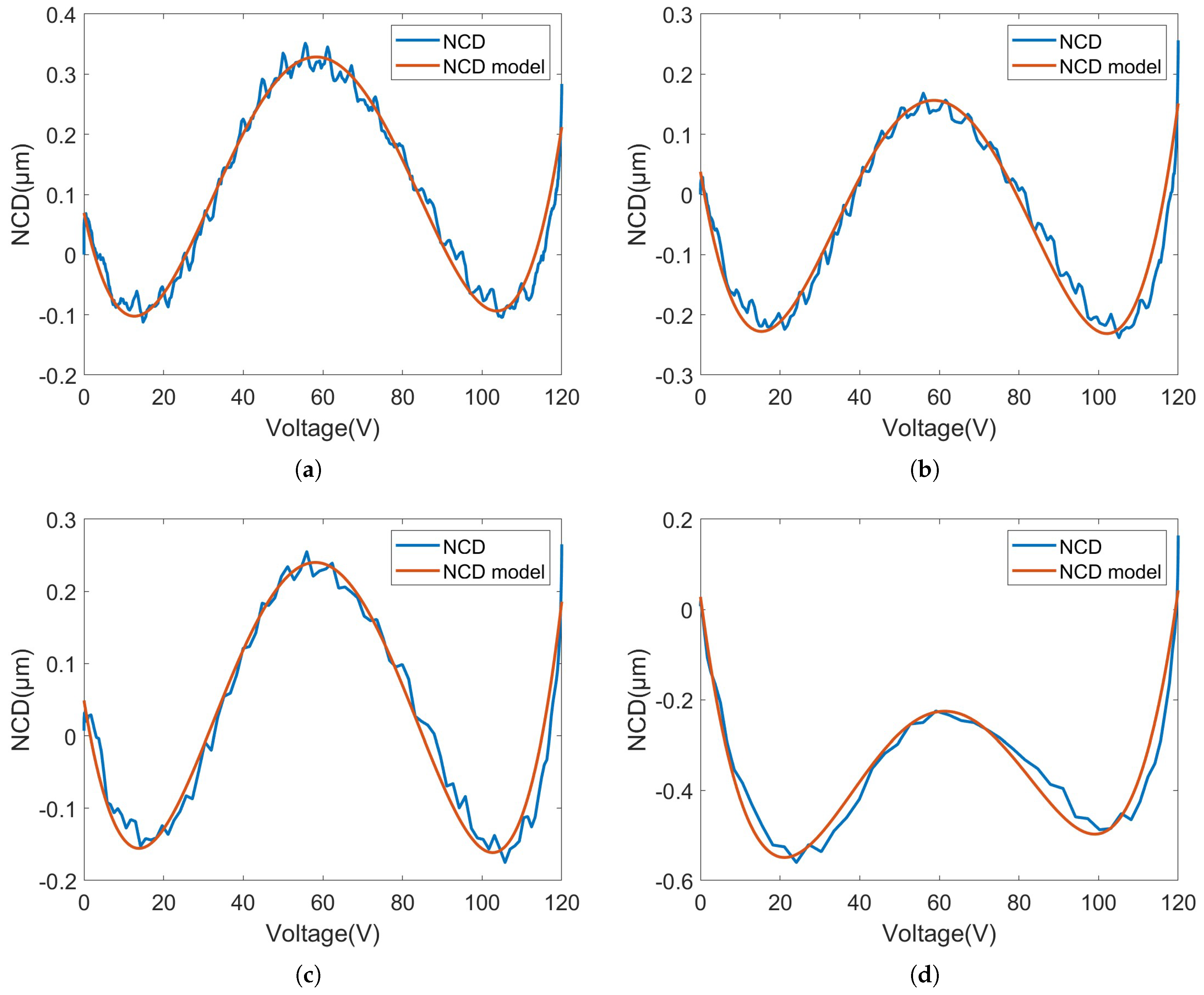
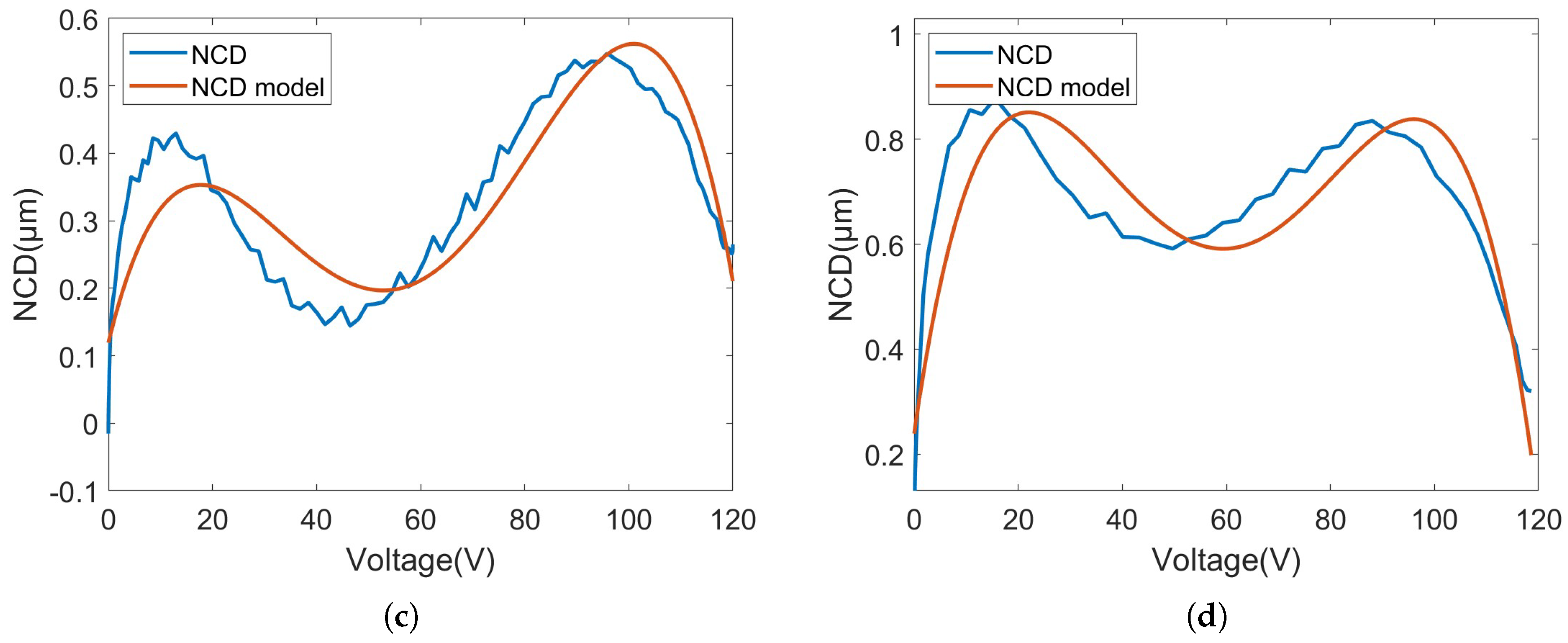
3.2.1. NCD Processor

The NCD processor is a dynamic compensation module specifically designed for piezoelectric actuators. Its core function is to output the NCD caused by speed changes by analyzing the velocity characteristics of a predetermined S-shaped trajectory driving voltage. This processor takes the instantaneous velocity of the S-shaped trajectory driving voltage as an input parameter, and the output NCD can be used for feedforward compensation to counteract dynamic positioning errors caused by velocity non-uniformity. By decomposing the nonlinear characteristics of the S-shaped trajectory into independently processable hysteresis and creep components, the NCD processor significantly improves the trajectory tracking accuracy of piezoelectric systems. The relationship curve between NCD and velocity is shown in Figure 4.

In practical applications, the NCD processor demonstrates clear regularity in the NCD separated from the S-shaped trajectory driving voltage of different frequencies. Experimental results show that as the velocity increases, the NCD exhibits a decreasing trend, which is consistent with the basic theory discussed earlier. Specifically, during the acceleration and deceleration phases of the boost phase, the NCD curves show a high degree of overlap, indicating that the piezoelectric actuator’s response is relatively consistent in these phases. However, during the acceleration and deceleration phases of the back phase, the NCD curves exhibit significant differences. This phenomenon is primarily due to the structural complexity of the piezoelectric actuator. In addition to the piezoelectric ceramic, the piezoelectric actuator also includes adhesive layers, electrode layers, and alumina protective layers. These materials inherently possess nonlinear elastic properties, especially the adhesive layer, which exhibits significant viscoelastic hysteresis and stress buffering effects during the back phase, leading to a larger NCD gap between the acceleration and deceleration phases. This phenomenon is consistent with recent research [30], further validating the theoretical foundation of the NCD processor.

In this analysis, macroscopic effects caused by materials and manufacturing processes are neglected, making the proposed capacitance change theory and NCD separation method reasonable. Through this simplification, the NCD processor can effectively separate the hysteresis and creep components in the S-shaped trajectory, thereby achieving precise control of the piezoelectric actuator. Additionally, the design of the NCD processor takes into account the dynamic response characteristics of the piezoelectric system, particularly the nonlinear effects under high-speed motion. Through feedforward compensation, the NCD processor can significantly reduce dynamic positioning errors caused by speed changes, further enhancing the overall performance of the system.

In summary, with its unique dynamic compensation mechanism, the NCD processor not only effectively decomposes the nonlinear characteristics in the S-shaped trajectory but also maintains high trajectory tracking accuracy under different velocity conditions. This technology provides a new solution for the application of piezoelectric actuators in high-precision positioning and control fields, offering broad application prospects.

3.2.2. NCD Model

On the basis of NCD separation, it is only necessary to convert it into a voltage value to achieve dynamic compensation for the piezoelectric actuator. Through the analysis in Section 3.1, it can be seen that the variation trend in NCD in both the boost and back phase exhibits a complex nonlinear characteristic of first increasing, then decreasing, then increasing again, and finally decreasing again. This variation trend is closely related to the dynamic response characteristics of the piezoelectric actuator, especially under high-speed motion or frequent acceleration and deceleration conditions, where the NCD variation becomes more significant. To accurately describe this nonlinear relationship, this paper adopts polynomial functions to model the boost and buck segments separately. Specifically, the relationship between NCD and voltage can be expressed by the following polynomial function:

$$d_{\mathrm{NCD}}=a_0+a_{1}v+a_2{v}^2+a_3{v}^3+a_4{v}^4$$

(12)

where $d_{\mathrm{NCD}}$ is the NCD value, v is the voltage value, and $a_i$ are the coefficients determined by experimental data fitting. This polynomial modeling method can effectively describe the nonlinear relationship between NCD and voltage, especially the complex variation trends of NCD in the boost and back phase.

Since polynomial functions themselves cannot be directly inverted, it is necessary to segment the NCD curve based on its extreme points. Specifically, the NCD curve can be divided into multiple monotonic intervals, and the polynomial function is inverted within each monotonic interval. This segmented inversion method effectively addresses the non-invertibility issue of polynomial functions while ensuring the accuracy of the inversion results. After segmented inversion, the obtained voltage value needs to be further divided by the sensitivity coefficient K of the piezoelectric actuator to obtain the actual compensation voltage value. The sensitivity coefficient K of the piezoelectric actuator is defined as the ratio of the steady-state displacement change $\mathrm{\Delta }x$ to the voltage change $\mathrm{\Delta }u$—i.e.,

$$K={\displaystyle \frac{\mathrm{\Delta }x}{\mathrm{\Delta }u}}$$

(13)

Therefore, the compensation voltage $u_{\mathrm{NCD}}$ can be calculated using the following formula:

$$u_{\mathrm{NCD}}={\displaystyle \frac{u}{K}}$$

(14)

where u is the voltage value obtained after segmented inversion, and K is the sensitivity coefficient of the piezoelectric actuator. Through this method, the NCD value can be converted into the actual compensation voltage value, thereby achieving precise control of the piezoelectric actuator.

In practical applications, for NCD generated by different predetermined trajectories, it is necessary to select appropriate mathematical modeling methods based on their characteristics. Although polynomial functions can effectively describe the nonlinear relationship between NCD and voltage, in some cases, higher-order polynomials or other nonlinear functions (such as exponential functions or piecewise linear functions) may be required to improve modeling accuracy. Additionally, for certain special motion trajectories, machine learning methods (such as neural networks or support vector machines) can be combined to model NCD, further enhancing the adaptability and prediction accuracy of the model.

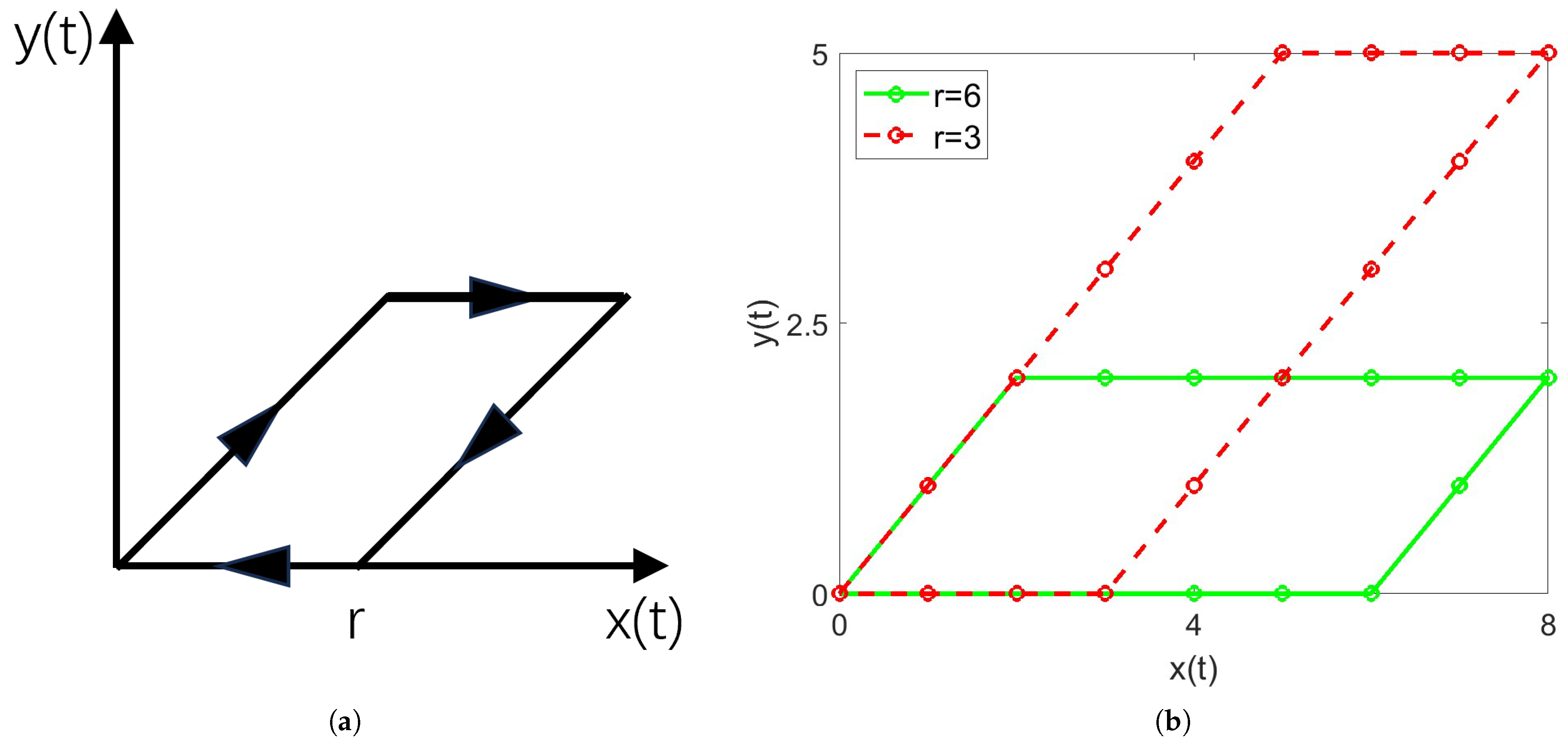
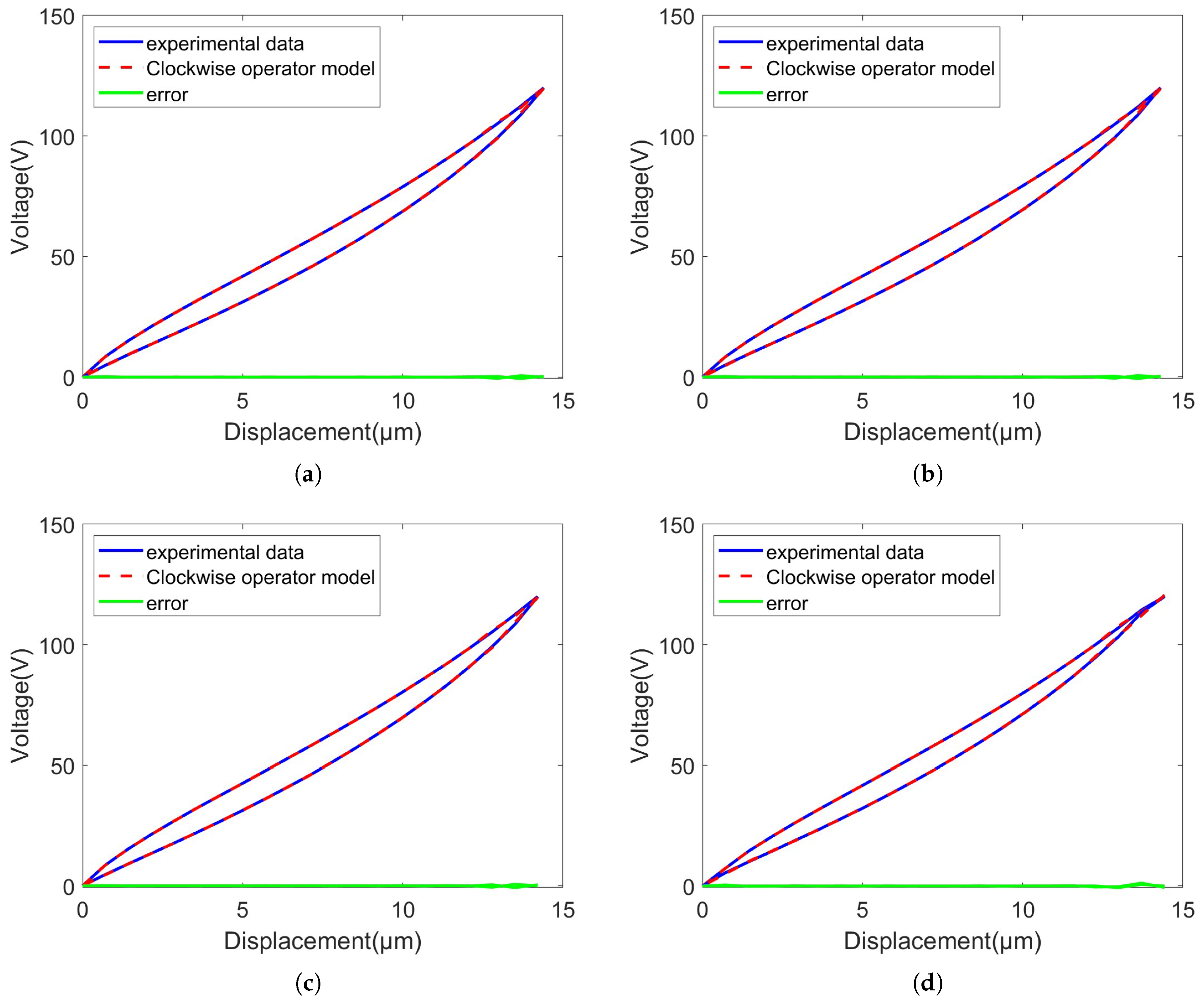
3.2.3. Clockwise Operator and Clockwise Operator Model

Apart from the NCD caused by speed change, piezoelectric actuators also have inherent hysteresis nonlinearity. To address this issue, this paper directly compensates for the displacement–voltage characteristics using the clockwise operator model, avoiding the problems of multiple control links and difficult inversion in the traditional feedforward control that requires modeling first and then inversion. The clockwise operator, as one of the fundamental operators of the clockwise operator model, describes the lead characteristics in the displacement–voltage nonlinearity of piezoelectric actuators. Since general piezoelectric actuators can only withstand positive voltage, this paper adopts a unilateral clockwise operator. The expression for the unilateral clockwise operator is as follows:

$$y\left(t\right)=\max \left(x\right(t)-r,\min (x\left(t\right),y(t+1)\left)\right)$$

(15)

$$y\left(n\right)=\max \left(x\right(n)-r,\min (x\left(n\right),y\left(n\right)\left)\right)$$

(16)

where $x\left(t\right)$ or $x\left(n\right)$ is the input of the unilateral clockwise operator at time t or n; $y\left(t\right)$ or $y\left(n\right)$ is the output of the unilateral clockwise operator at time t or n; and r is the threshold of the unilateral clockwise operator. Figure 5a is a schematic diagram of the unilateral clockwise operator, illustrating the relationship between the input $x\left(t\right)$ and the output $y\left(t\right)$.

When the threshold $r=6$, the input and output are $x\left(t\right)$ and $y\left(t\right)$, respectively; when the threshold $r=3$, the input and output are $x_1\left(t\right)$ and $y_1\left(t\right)$, respectively. Using MATLAB-2022a to compute the unilateral clockwise operator, the unilateral clockwise operator plots for the same input but different thresholds are shown in Figure 5b.

The unilateral clockwise operator output continues to increase at the same rate as the input until it reaches a point where the input distance is less than the threshold. At this point, the clockwise operator output begins to remain constant. When the input value reaches its maximum, the unilateral clockwise operator output starts to decrease at the same rate until the input returns to the threshold. At this stage, the unilateral clockwise operator output continues to remain unchanged, ultimately forming a closed loop.

The clockwise operator model is derived by performing a weighted summation of different unilateral clockwise operators. Its specific expression is as follows:

$$y\left(t\right)=H[x\left(t\right),y(t+1)]=\sum _{k=1}^n{\omega }_i^{*}\left(t\right)\max (x\left(t\right)-r,\min (x\left(t\right),y(t+1)))$$

(17)

where $H[·]$ represents the lead relationship. $x\left(t\right)$ and $y\left(t\right)$ are the input and output of the advanced prediction model, respectively. The weight vector is ${\omega }^{*}\left(t\right)={({\omega }_1^{*}\left(t\right),\dots ,{\omega }_n^{*}\left(t\right))}^T$. The threshold vector is $r={(r_1,\dots ,r_n)}^T$. The final-state vector of unilateral advanced operators is $y\left[n\right]={(y_1\left[n\right],\dots ,y_n\left[n\right])}^T$.

The problem of obtaining a suitable clockwise operator model for system nonlinearity depends on selecting an appropriate set of thresholds and then determining the coefficients that best fit the nonlinear curve associated with this set. This can be achieved using parameter estimation algorithms such as Particle Swarm Optimization (PSO). However, to obtain a more accurate model, a large number of unilateral clockwise operators are required, each with a coefficient that needs to be fitted. This results in a vast optimization space, which in many cases leads to slow convergence. Fortunately, the coefficient values can be derived by studying the geometry of the clockwise operator model.

Considering an ordered set $\left\{r_i\right\}$, where $r_i<r_{i+1}$, representing the thresholds of the unilateral clockwise operator that constitute the clockwise operator model. Now, consider the input–output curve segment of the clockwise operator model described by Equation (15), where the input values lie between two consecutive thresholds $u=u_{\max }-r_i$ and $u=u_{\max }-r_{i+1}$. This segment of the curve is a superposition of unilateral clockwise operators. However, all clockwise operators with thresholds smaller than $r_i$ have not yet closed because the input is not large enough. This implies that none of the clockwise operators with thresholds smaller than $r_i$ contribute to the curve segment between $u=u_{\max }-r_i$ and $u=u_{\max }-r_{i+1}$. On the other hand, all clockwise operators with thresholds lower than $r_{i+1}$ will be active on this segment.

As shown in Figure 6, once the input increases to less than the maximum input minus the threshold of the clockwise operators constituting the clockwise operator model, their output will increase at the same rate as the input and can be described by a line segment with unit slope. However, as indicated by Equation (15), the coefficient ${\omega }_i$ modifies the slope of this line segment. This holds true for all clockwise operators constituting the clockwise operator model, meaning that the segment between two consecutive thresholds is a superposition of line segments and must itself be a line segment. The slope $k_i$ between the inputs $u=u_{\max }-r_i$ and $u=u_{\max }-r_{i+1}$ can be described solely by the coefficients as shown in Equation (16). Using this equation, the problem of estimating the coefficients is reduced to finding the slope of the line segment that best fits the system between consecutive threshold inputs.

$$k_i=\sum _{j=1}^i{\omega }_j$$

(18)

3.3. Hybrid Control Strategy Combining Nonlinear Compensation and Trajectory Shaping

Under the S-shaped trajectory driving voltage, the nonlinear characteristics of piezoelectric actuators manifest as the combined effect of their inherent hysteresis nonlinearity and NCD caused by speed changes. This complex nonlinear characteristic can lead to significant deviations between the actual motion trajectory of the actuator and the predetermined trajectory, seriously affecting the performance of high-precision positioning systems. To address this issue, this paper proposes a hybrid control strategy that combines nonlinear compensation and trajectory shaping. The control block diagram is shown in Figure 6. The core of this strategy lies in the step-by-step processing of the nonlinear characteristics of piezoelectric actuators and the use of model-driven compensation methods to effectively suppress complex nonlinearity.

Firstly, the hysteresis characteristics of the piezoelectric actuator are calibrated through experiments, and its hysteresis model is established. On this basis, the motion data of the piezoelectric actuator at different speeds are analyzed using an NCD processor to separate the NCD values caused by speed changes. The NCD processor decouples the dynamic response of the input signal, extracts creep components related to velocity, and quantifies them into specific NCD values. Subsequently, a corresponding compensation voltage is generated based on the NCD model, which can effectively counteract the non-uniform creep effect caused by speed changes. At the same time, by bringing in the output of the clockwise operator model, hysteresis nonlinear compensation and NCD compensation are combined to generate a synthesized voltage applied to the piezoelectric actuator.

It is worth noting that through the analysis of the displacement voltage characteristics of piezoelectric actuators, it is known that they have asymmetry, while the output of the general clockwise operator model is a symmetrical model. To improve the accuracy of the model, this paper models the displacement–voltage characteristics of piezoelectric actuators in segments based on the law of velocity deformation. In the modeling process, the complete clockwise operator was not used, but the clockwise operator was selected based on the principle of concave convex consistency. This means that in nonlinear curves, the convex curve of the boosting part and the concave curve of the lowering part use the corresponding unilateral operator. The specific operation steps are as follows:

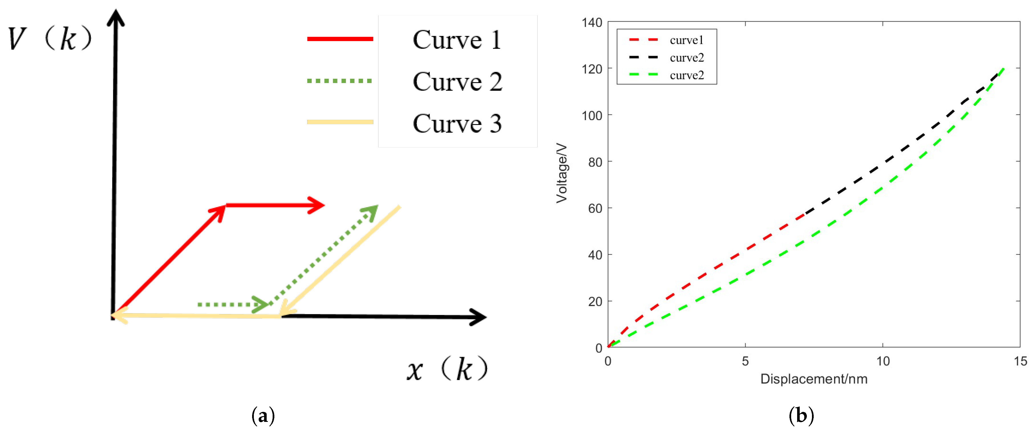
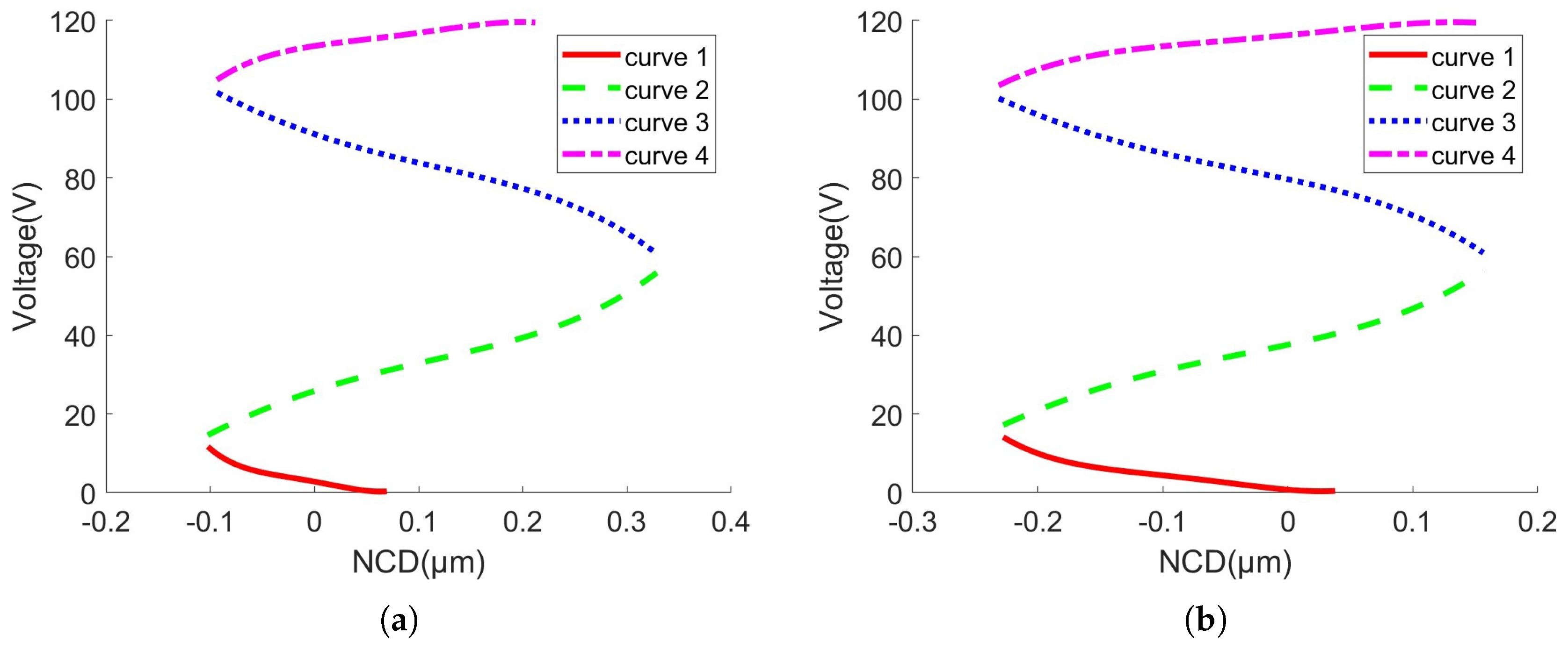
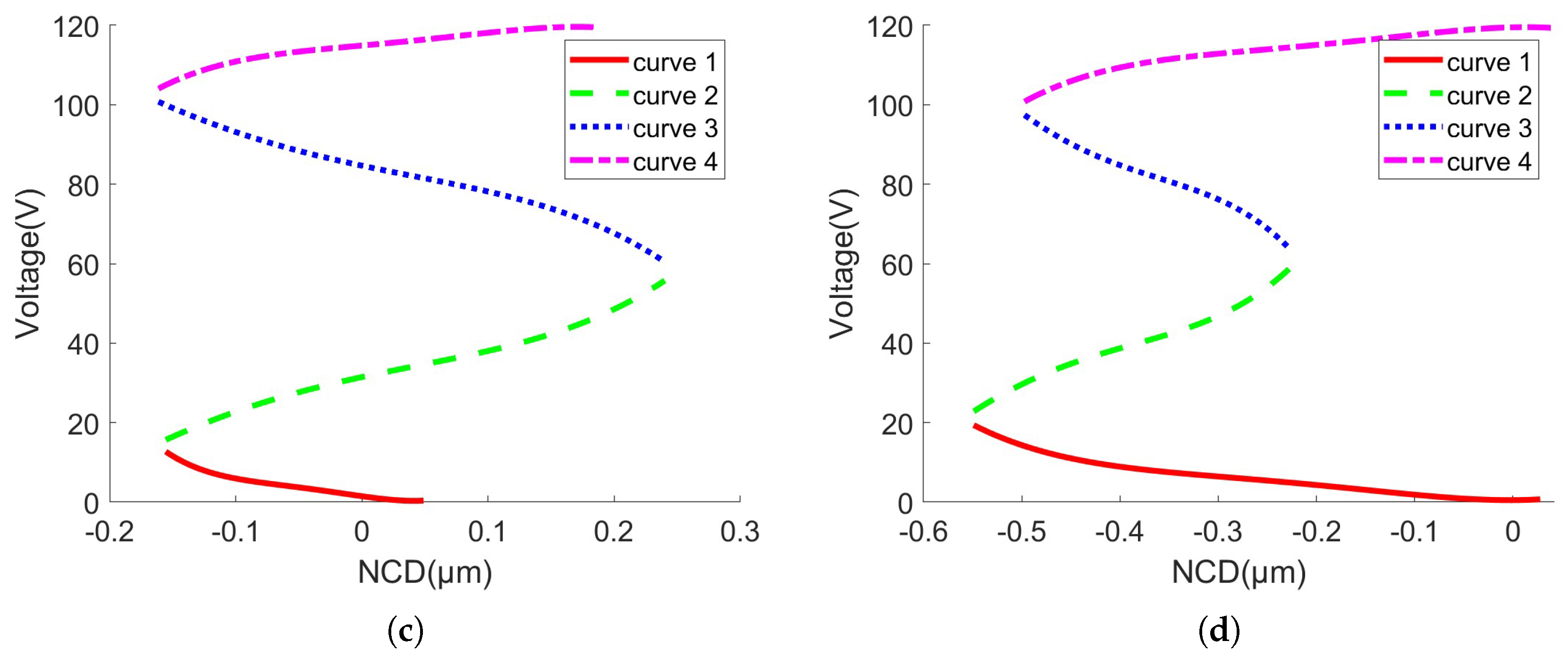
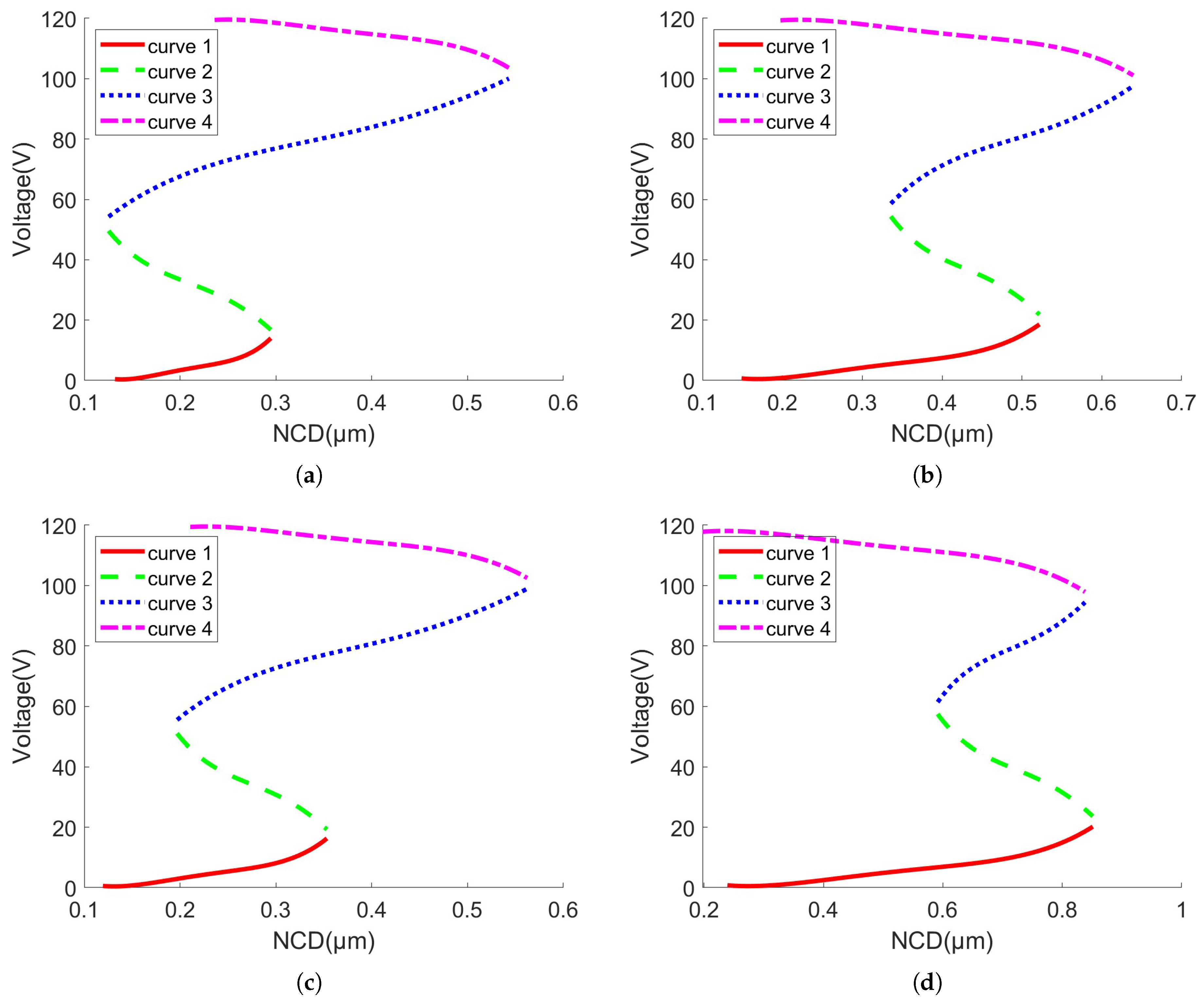
• First Segment (Rising Curve from Zero Displacement to the Inflection Point);
  The inflection point is determined based on the fuzzy selection of voltage rate. When the voltage rises from 0 to the minimum rate, the relationship between voltage and displacement is described by a unilateral operator, as shown by curve 1 in Figure 7a.
• Second Segment (Rising Curve from the Inflection Point to the Maximum Displacement);
  In this segment, the relationship between voltage and displacement is described by another unilateral operator, as shown by curve 2 in Figure 7a. During the displacement increase, the voltage rate also increases, which exhibits a trend opposite to the falling unilateral process of the clockwise operator. Therefore, a reverse falling unilateral clockwise operator is used for special modeling in this segment.
• Third Segment (Falling Curve from Maximum Displacement to Zero Displacement).

The relationship between voltage and displacement during this phase is described by another unilateral operator, as shown by curve 3 in Figure 7a.

The weight and threshold selection method is consistent with the general clockwise operator model. The final synthesis result of the segmented clockwise operator model modeling is shown in Figure 7b. From the analysis in Figure 7b, the segmented aclockwise operator model exhibits asymmetry, and its concavity and convexity are consistent with the displacement voltage characteristics of the piezoelectric ceramic actuator.

The advantage of this hybrid control strategy is that it can not only dynamically compensate for the NCD caused by speed changes through the NCD model, but also accurately compensate for the inherent hysteresis characteristics of the piezoelectric actuator through a clockwise operator model. Through the synergistic effect of the two, the synthesized voltage can significantly reduce the deviation between the actual motion trajectory and the predetermined trajectory, thereby improving the control accuracy and trajectory tracking performance of the system. This strategy exhibits good robustness and adaptability at different speeds, providing an effective solution for nonlinear control of high-precision piezoelectric actuation systems.

4. Experiments and Discussion

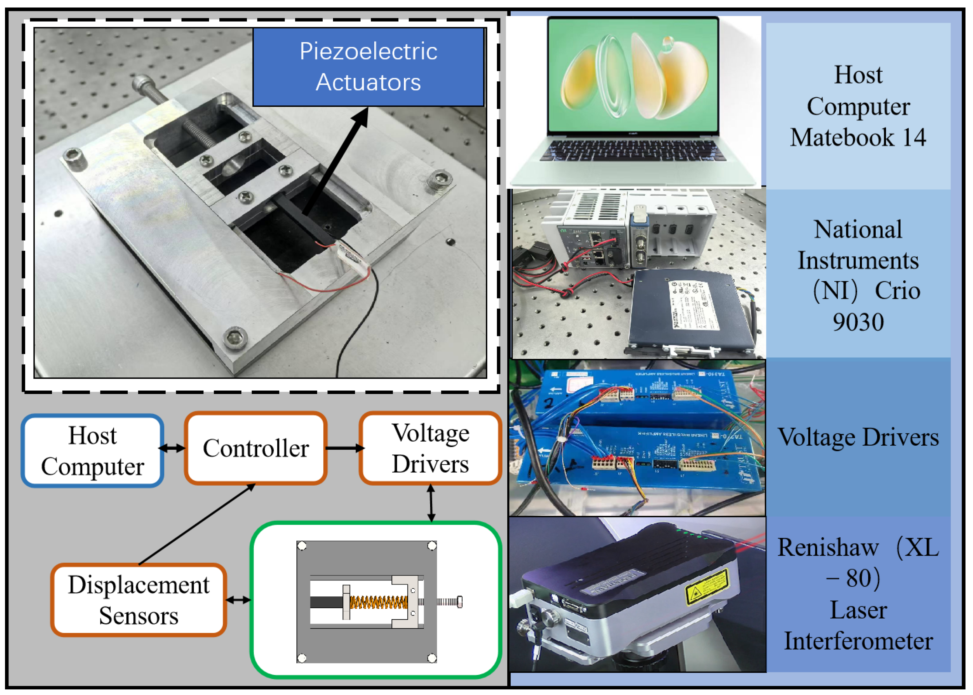
4.1. Experimental Setup

To verify the feedforward control strategy of the clockwise operator model based on considering NCD characteristics proposed in this article, the hardware system of the optimized fourth-order actuation experimental platform mainly consists of a controller and multi-channel linear actuators.

The functional testing platform is a one-dimensional piezoelectric actuation platform, whose function is completely equivalent to that of a lathe tool platform. A Renishaw XL-80 laser interferometer from England was selected as the displacement sensor. We also used theNational Instruments (NI) crio 9030 real-time controller from America. The entire experimental platform was built as shown in Figure 8.

The functional test platform utilizes a bolt and spring assembly to preload the piezoelectric actuator, with the addition of a guide block to ensure that the motion direction of the piezoelectric actuator remains consistent. A load platform is positioned between the piezoelectric actuator and the spring to secure the reflector, enabling displacement measurement. The specific functional test platform is illustrated in Figure 9. The piezoelectric actuator is driven by a linear power amplifier, and its displacement is measured using a laser interferometer.

The piezoelectric actuator is fabricated from lead zirconate titanate (PbZrTiO₃, PZT) piezoelectric ceramic material, which exhibits a large piezoelectric charge coefficient, moderate dielectric constant, and high electromechanical coupling coefficient. Furthermore, the piezoelectric actuator (7 mm × 7 mm × 18 mm) is constructed by stacking multiple piezoelectric ceramic layers, and the input voltage is typically maintained as positive to preserve the actuator’s performance.

4.2. Separation Results from Model Identification Results

The NCD separation method is used to separate the NCD values in the nonlinear features under the S-shaped trajectory driving voltage, as shown in Figure 10.

Figure 11 clearly shows the specific NCD separated from the experimental data. As shown in Figure 11, the extracted NCD values exhibit consistent trends at different frequencies, which is highly consistent with theoretical expectations and previous analysis results. This consistency not only validates the reliability of the NCD separation method, but also highlights the robustness and adaptability of the proposed method under different operating conditions. Specifically, under driving signals of different frequencies, the separation results of NCD values show similar regular changes, indicating that this method can effectively capture the NCD effect caused by speed changes and is not significantly affected by frequency changes.

In addition, this consistency further demonstrates the universality of the NCD separation method. No matter how the frequency of the driving signal changes, the extraction process of the NCD value can maintain high accuracy and stability, which provides a reliable data basis for subsequent nonlinear compensation. At the same time, the experimental results also indicate that the proposed method can effectively address the various working conditions that piezoelectric actuators may encounter in practical applications, providing theoretical support and technical support for their application in high-precisiono positioning systems.

The modeling results of NCD under different frequency S-shaped trajectory driving voltages using the polynomial method are shown in the figure. Note that the modeling process should focus on separately modeling the boost and back phase. Figure 12 is the NCD model in the boost phase and Figure 13 is the NCD model in the back phase.

We used the least-squares optimization algorithm to identify the parameters in Formula (12) [31]. The parameters are shown in

Table 3. Parameter table of NCD model in boost phase.

Frequency	${\mathit{a}}_0$	${\mathit{a}}_1$	${\mathit{a}}_2$	${\mathit{a}}_3$	${\mathit{a}}_4$
0.25 Hz	9.9565 $\times {10}^{-8}$	−2.3243 $\times {10}^{-5}$	0.0016	−0.0305	0.0694
0.5 Hz	1.1026 $\times {10}^{-7}$	−2.5842 $\times {10}^{-5}$	0.0019	−0.0403	0.0385
1 Hz	1.0219 $\times {10}^{-7}$	−2.3784 $\times {10}^{-5}$	0.0017	−0.0336	0.0489
2 Hz	1.2875 $\times {10}^{-7}$	−3.1169 $\times {10}^{-5}$	0.0024	−0.0661	0.0279

:

The parameters obtained using the same optimization method are shown in

Table 4. Parameter table of NCD model in back phase.

Frequency	${\mathit{a}}_0$	${\mathit{a}}_1$	${\mathit{a}}_2$	${\mathit{a}}_3$	${\mathit{a}}_4$
0.25 Hz	$-7.7840\times {10}^{-8}$	1.7520 $\times {10}^{-5}$	−0.0012	0.0249	0.1321
0.5 Hz	$-9.9332\times {10}^{-8}$	2.3277 $\times {10}^{-5}$	−0.0017	0.0449	0.1484
1 Hz	$-8.2943\times {10}^{-8}$	1.8969 $\times {10}^{-5}$	−0.0013	0.0314	0.1194
2 Hz	$-1.1929\times {10}^{-7}$	2.2908 $\times {10}^{-5}$	−0.0023	0.0661	0.2259

:

Figure 14 and Figure 15 show the inverses of the NCD models. Since the NCD model cannot be directly inverted, it can be segmented based on its extremum points. The curves 1–4 in the figure represent the inverse of each segment.

4.3. Experimental Results

The clockwise operator model and the PI model have the same function in this article; both are used to describe the hysteresis characteristics of the system and achieve precise control. However, the innovation of this article lies in the introduction of the consideration of NCD caused by speed changes, which has not been fully considered in previous studies. By incorporating NCD into the model design, this paper allows for more comprehensively capturing the nonlinear behavior of the system, thereby improving control accuracy and robustness. In contrast, most existing studies rely solely on linearization assumptions or ignore the influence of nonlinear factors, which may result in limitations of the model in practical applications. This study not only fills this gap, but also provides new ideas and methods for further exploration in related fields. The output and error of the clockwise operator model are shown in Figure 16.

In this paper, an appropriate threshold is selected, and the least-squares method is employed to optimize the weights [30]. The results of threshold and weight values are shown in Appendix B.

Below are the relevant translations and explanations of the formulas and calculation results:

Maximum Relative Error (MRE):

$$e_{\max }(\%)={\displaystyle \frac{\max \left(\right|e\left|\right)}{\max \left(x_d\right)-\min \left(x_d\right)}}\times 100\%$$

(19)

Maximum Mean Square Error(MMSE):

$$e_{\max }(\%)={\displaystyle \frac{\sqrt{\frac{1}{N}{\sum }_{i=1}^N{e}_i^2}}{\max \left(x_d\right)-\min \left(x_d\right)}}\times 100\%$$

(20)

The specific results are shown in

Table 5. Error evaluation value.

	0.25 Hz	0.5 Hz	1 Hz	2 Hz
MRE	3.89%	4.89%	5.48%	4.78%
MMSE	0.11%	0.12%	0.15%	0.28%

.

5. Conclusions

This paper proposes a hybrid compensation method to address the mixed nonlinearities of piezoelectric actuated machine tools (PAMTs) under S-shaped trajectory driving voltage. Based on capacitance theory, the relationship between speed change and actuator deformation was analyzed, leading to a non-uniform creep difference (NCD) processor. NCD and hysteresis were modeled using a polynomial model and a clockwise operator model. Subsequently, a hybrid feedforward control strategy integrating these models effectively mitigated velocity-dependent NCD and inherent hysteresis. The experimental results show that the maximum MRE and MMSE of this method are 5.48% and 0.28%, respectively, and the modeling accuracy is improved by about 70% compared with the NCD uncompensated model. The S-shaped trajectory tracking accuracy was significantly improved.

This method not only improves the control accuracy of PAMTs, but also applies to other piezoelectric devices such as cell probes, especially in the case of combined motion trajectories. The clockwise operator model simplifies hysteresis modeling and reduces computational complexity by directly dealing with inverse relationships, and can also be used with other control algorithms. Future work will focus on developing a real-time strategic workflow, from automated analysis of NCD trends and model building to adaptive optimization of voltage compensation drives, to the integration of piezo actuator output performance under special conditions. Therefore, it is possible to extend the applicability of this hybrid compensation method to a wider range of applications.

References

1. Zhang, F.; Zhang, C.; Zhang, L.; Cheng, R.; Li, R.; Pan, Q.; Huang, Q. Hysteresis segmentation modeling and experiment of piezoelectric ceramic actuator. IEEE Sens. J. 2022, 4, 21153–21162. [Google Scholar] [CrossRef]
2. Yang, L.; Zhang, Y.; Zhao, Z.; Li, D. Fractional-order control for nano-positioning of piezoelectric actuators. Int. J. Mod. Phys. B 2022, 7, 2250134. [Google Scholar] [CrossRef]
3. Li, C.X.; Gu, G.Y.; Yang, M.J.; Zhu, L.M. High-speed tracking of a nanopositioning stage using modified repetitive control. IEEE Trans. Autom. Sci. Eng. 2015, 5, 1467–1477. [Google Scholar] [CrossRef]
4. Zhao, D.; Zhu, Z.; Huang, P.; Guo, P.; Zhu, L.; Zhu, Z. Development of a piezoelectrically actuated dual-stage fast tool servo. Mech. Syst. Signal Process. 2020, 144, 106873. [Google Scholar] [CrossRef]
5. Liu, Y.T. Recent development of piezoelectric fast tool servo (FTS) for precision machining. Int. J. Precis. Eng. Manuf. 2024, 25, 851–874. [Google Scholar] [CrossRef]
6. Xu, A.; Gu, Q.; Yu, H. Mechanism of controllable force generated by coupling inverse effect of piezoelectricity and magnetostriction. Int. J. Precis. Eng. Manuf. Green Technol. 2021, 144, 1297–1307. [Google Scholar] [CrossRef]
7. Malayath, G.; Mote, R.G. A review of cutting tools for ultra-precision machining. Mach. Sci. Technol. 2022, 26, 923–976. [Google Scholar]
8. Liu, H.; Lai, X.; Wu, W. Time-optimal and jerk-continuous trajectory planning for robot manipulators with kinematic constraints. Robot. Comput. Integr. Manuf. 2013, 29, 309–317. [Google Scholar] [CrossRef]
9. Han, C.J.; Song, K.R.; Rim, U.R. An asymmetric S-curve trajectory planning based on an improved jerk profile. Robotica 2024, 42, 2184–2208. [Google Scholar] [CrossRef]
10. Mahale, B.; Kumar, N.; De, A.; Pandey, R.; Ranjan, R. A comparative study of energy harvesting performance of polymer-piezoceramic composites fabricated with different piezoceramic constituents. Int. J. Energy Res. 2020, 9, 2694–2708. [Google Scholar] [CrossRef]
11. Tao, H.; Wu, J. New poling method for piezoelectric ceramics. J. Mater. Chem. C 2017, 5, 1601–1606. [Google Scholar] [CrossRef]
12. Gu, G.Y.; Zhu, L.M.; Su, C.Y.; Ding, H.; Fatikow, S. Modeling and control of piezo-actuated nanopositioning stages: A survey. IEEE Trans. Autom. Sci. Eng. 2014, 13, 313–332. [Google Scholar] [CrossRef]
13. Kanchan, M.; Santhya, M.; Bhat, R.; Naik, N. Application of modeling and control approaches of piezoelectric actuators: A review. Technologies 2023, 11, 155. [Google Scholar] [CrossRef]
14. Li, P.Z.; Wang, X.D.; Zhao, L.; Zhang, D.F.; Guo, K. Dynamic linear modeling, identification and precise control of a walking piezo-actuated stage. Mech. Syst. Signal Process. 2019, 128, 141–152. [Google Scholar] [CrossRef]
15. Al Janaideh, M.; Al Saaideh, M.; Tan, X. The Prandtl–Ishlinskii hysteresis model: Fundamentals of the model and its inverse compensator [Lecture Notes]. IEEE Control Syst. Mag. 2023, 43, 66–84. [Google Scholar] [CrossRef]
16. Baziyad, A.G.; Ahmad, I.; Salamah, Y.B. Precision Motion Control of a Piezoelectric Actuator via a Modified Preisach Hysteresis Model and Two-Degree-of-Freedom H-Infinity Robust Control. Micromachines 2023, 6, 1208. [Google Scholar] [CrossRef] [PubMed]
17. Xu, M.; Su, L.; Chen, S. Improved PI hysteresis model with one-sided dead-zone operator for soft joint actuator. Sens. Actuators A Phys. 2022, 12, 114072. [Google Scholar] [CrossRef]
18. Yang, L.; Wang, Q.; Xiao, Y.; Li, Z. Hysteresis modeling of piezoelectric actuators based on a TS fuzzy model. Electronics 2022, 11, 2786. [Google Scholar] [CrossRef]
19. Garra, R.; Mainardi, F.; Spada, G. A generalization of the Lomnitz logarithmic creep law via Hadamard fractional calculus. Chaos Solitons Fractals 2017, 102, 333–338. [Google Scholar] [CrossRef]
20. Dogruer, C.U.; Yıldırım, B. Multiple Model Switching Control of Linear Time-Invariant Systems. Chaos Solitons Fractals 2024, 49, 10961–10975. [Google Scholar] [CrossRef]
21. Liu, Y.; Shan, J.; Qi, N. Creep modeling and identification for piezoelectric actuators based on fractional-order system. Mechatronics 2013, 49, 840–847. [Google Scholar] [CrossRef]
22. Jung, H.; Shim, J.Y.; Gweon, D.G. New open-loop actuating method of piezoelectric actuators for removing hysteresis and creep. Rev. Sci. Instrum. 2000, 71, 3436–3440. [Google Scholar] [CrossRef]
23. Nie, Z.; Cui, Y.; Huang, J.; Wang, Y.; Chen, T. Precision open-loop control of piezoelectric actuator. J. Intell. Mater. Syst. Struct. 2022, 33, 1198–1214. [Google Scholar] [CrossRef]
24. Ru, C.; Sun, L. Hysteresis and creep compensation for piezoelectric actuator in open-loop operation. Sens. Actuators A Phys. 2005, 122, 124–130. [Google Scholar]
25. Krejci, P.; Kuhnen, K. Inverse control of systems with hysteresis and creep. IEE Proc. Control Theory Appl. 2001, 148, 185–192. [Google Scholar] [CrossRef]
26. Kuhnen, K.; Janocha, H. Operator-based compensation of hysteresis, creep and force-dependence of piezoelectric stack actuators. IFAC Proc. Vol. 2000, 33, 407–412. [Google Scholar] [CrossRef]
27. Mokaberi, B.; Requicha, A.A.G. Compensation of scanner creep and hysteresis for AFM nanomanipulation. IEEE Trans. Autom. Sci. Eng. 2008, 5, 197–206. [Google Scholar] [CrossRef]
28. Yang, Q.; Jagannathan, S. Creep and hysteresis compensation for nanomanipulation using atomic force microscope. Asian J. Control 2009, 11, 182–187. [Google Scholar] [CrossRef]
29. Huang, L.C.; Fu, C.M. Spontaneous polarization and dielectric relaxation dynamics of two novel diastereomeric ferroelectric liquid crystals. Acta Phys. Pol. A 2016, 129, 97–102. [Google Scholar] [CrossRef]
30. Kang, H.; Shu, F.; Li, Z.; Yang, X. Modeling of bonding piezoelectric stack using conductive adhesive with metal-coated polymer fillers. Mech. Syst. Signal Process. 2023, 194, 110138. [Google Scholar] [CrossRef]
31. Zhang, K.; Yang, P.Y.; Shi, H.T.; Guo, J. Fault detection method based on improved dynamic partial least square method. J. Shenyang Jianzhu Univ. Sci. 2024, 40, 167–178. [Google Scholar]
Figure 1. Typical structure of PAMT.
Applsci 15 04207 g001
Figure 2. Complex nonlinear characteristics of piezoelectric actuators under S-shaped trajectory driving voltage: (a) 0.25 Hz. (b) 0.5 Hz. (c) 1 Hz. (d) 2 Hz.
Applsci 15 04207 g002
Figure 3. S-shaped trajectory driving voltage and triangular wave driving voltage: (a) 0.25 Hz. (b) 0.5 Hz. (c) 1 Hz. (d) 2 Hz.
Applsci 15 04207 g003
Figure 4. The relationship curve between NCD and velocity: (a) 0.25 Hz. (b) 0.5 Hz. (c) 1 Hz. (d) 2 Hz.
Applsci 15 04207 g004
Figure 5. Diagram and simulation of clockwise operator: (a) Diagram of clockwise operator. (b) Simulation of clockwise operator.
Applsci 15 04207 g005
Figure 6. Block diagram of composite nonlinear feedforward control strategy.
Applsci 15 04207 g006
Figure 7. Segmented clockwise operator and model: (a) Segmented clockwise operator. (b) Segmented clockwise operator model.
Applsci 15 04207 g007
Figure 8. Experimental setup.
Applsci 15 04207 g008
Figure 9. The functional test platform.
Applsci 15 04207 g009
Figure 10. The separation of NCD: (a) 0.25 Hz. (b) 0.5 Hz. (c) 1 Hz. (d) 2 Hz.
Applsci 15 04207 g010
Figure 11. NCD: (a) 0.25 Hz. (b) 0.5 Hz. (c) 1 Hz. (d) 2 Hz.
Applsci 15 04207 g011
Figure 12. NCD model in boost phase: (a) 0.25 Hz. (b) 0.5 Hz. (c) 1 Hz. (d) 2 Hz.
Applsci 15 04207 g012
Figure 13. NCD model in back phase: (a) 0.25 Hz. (b) 0.5 Hz. (c) 1 Hz. (d) 2 Hz.
Applsci 15 04207 g013aApplsci 15 04207 g013b
Figure 14. Inverse of NCD model in boost phase: (a) 0.25 Hz. (b) 0.5 Hz. (c) 1 Hz. (d) 2 Hz.
Applsci 15 04207 g014aApplsci 15 04207 g014b
Figure 15. Inverse of NCD model in back phase: (a) 0.25 Hz. (b) 0.5 Hz. (c) 1 Hz. (d) 2 Hz.
Applsci 15 04207 g015
Figure 16. Clockwise operator model: (a) 0.25 Hz. (b) 0.5 Hz. (c) 1 Hz. (d) 2 Hz.
Applsci 15 04207 g016