Cold Wave Recognition and Wind Power Forecasting Technology Considering Sample Scarcity and Meteorological Periodicity Characteristics

Abstract

Accurate recognition of both cold wave occurrence and wind power during cold wave events is critically significant to ensure the stable operation of the power system under extreme meteorological conditions. In view of the above problems, this paper proposes a cold wave event recognition method and a day-ahead wind farm cluster power forecasting model. In order to effectively recognize cold wave events, this paper proposes a cold wave discrimination criterion based on wind turbine operation characteristics and NWP data. The proposed recognition criterion employs seasonal meteorological features processed through a GAN-enhanced multi-modal U-Net architecture, effectively mitigating sample scarcity issues. To improve the forecasting accuracy of wind farm cluster power during cold wave events, a combined forecasting model based on the Ns-Transformer model is constructed by combining NWP data with cold wave recognition results. A wind farm cluster is taken as an example to verify the effectiveness of the proposed method. Compared to that of LSTM, Random Forest, BP, and Transformer models, the RMSE of the proposed method is reduced by 5.65%, 5.58%, 4.81%, and 0.44%, respectively, during cold wave occurrence seasons. The results show that the proposed method is superior to the conventional method in terms of cold wave recognition ability and wind power forecasting accuracy.

1. Introduction

With the depletion of global fossil energy and the increasingly prominent environmental issues, the proportion of wind power in the energy mix has increased [1]. By December 2024, China’s cumulative installed power capacity was about 3.35 TW, with installed wind power capacity reaching approximately 520 GW, an 18.0% increase year-on-year [2]. However, the growth in wind power capacity significantly impacts the stable operation of the power system [3]. In recent years, extreme cold wave events have occurred intermittently against the backdrop of global climate change. Cold wave events are often characterized by a sudden drop in temperature and a sharp increase in wind speed [4]. When such weather occurs in areas with large-scale wind farms, the fluctuation and uncertainty of wind power generation increase, and in severe cases, may cause widespread issues such as wind turbine shutdowns and units going off-grid [5,6]. The 2021 Texas power crisis was directly caused by prolonged extreme cold wave events, resulting in a lack of sustainable power supply from renewable energy sources and power outages, affecting more than 4.5 million customers [7]. Therefore, accurate forecasting of cold wave events and wind power forecasting during such conditions is crucial for the stable operation of the power system under extreme weather conditions [8].

In recent years, forecasting methods that effectively model the complex nonlinear relationships in data have been widely used in wind power forecasting [9,10]. Methods such as Empirical Mode Decomposition (EMD) [11,12,13], wavelet transform [14], and principal component analysis [15] are used to capture the complex interdependencies between variables. Genetic Algorithms (GAs) [16] and particle swarm optimization (PSO) algorithms [17,18] have been applied to optimize the parameters of forecasting models. Additionally, methods that modify Numerical Weather Prediction (NWP) by incorporating the spatiotemporal characteristics of wind power features [19,20] can significantly improve forecasting accuracy. However, regular weather forecasting methods cannot capture power changes during extreme weather events.

To enhance wind power forecasting accuracy under extreme weather conditions, reference [21] proposed a short-term forecasting methodology incorporating the recognition and verification of transitional weather processes. The approach employs an object-oriented diagnostic verification method to analyze wind speed sequences during transitional weather, extracting NWP forecast patterns for extreme meteorological events. Transitional weather is primarily characterized by abrupt fluctuations in power output, while cold-wave conditions mainly lead to wind power losses, demonstrating the distinct impacts of these two weather scenarios on wind power generation. Reference [22] developed a dual-adaptive sliding window inflection point detection method for extracting transitional power periods, effectively identifying wind power ramp events during extreme weather. Current research predominantly focuses on characterizing and detecting ramp events, yet singular ramp forecasting proves inadequate for cold wave scenarios given the diversity of extreme weather types. Existing studies have improved wind power forecasting accuracy under extreme weather conditions through scenario classification methods. However, their scenario-partitioning mechanisms still exhibit significant limitations. For instance, some studies classify NWP data into different scenarios based on wind speed and wind direction [23]. Additionally, one study categorized scenarios into low-temperature shutdown, high-wind cutoff, and icing-induced derating based on different mechanisms by which low-temperature cold waves affect wind power shutdown [24]. Scenario classification enhances the adaptability of forecasting models to different types of extreme weather. However, most scenario classifications rely on the statistical characteristics of wind power operation states or the clustering of shallow meteorological parameters, failing to fully integrate the intrinsic physical correlations among multidimensional NWP variables. Moreover, the refinement of scenario identification remains insufficient, with inadequate criteria for scenario assessment, leading to blurred scenario boundaries and reduced generalization when predicting future scenarios.

Cold wave events are a small-sample scenario in wind power forecasting, where data scarcity impedes effective model learning of their characteristic patterns. To address sample sparsity challenges, researchers have implemented small-sample augmentation [25,26,27] and transfer learning approaches [28,29]. Reference [25] establishes meteorological criteria for cold wave recognition and the analysis of wind power generation characteristics. Specifically targeting data scarcity in cold wave modeling, the Time-GAN algorithm has been employed to synthesize enhanced meteorological and power operational datasets. Recent advancements integrate wind turbine physics with data augmentation techniques to enhance forecasting robustness [30,31,32]. The authors of [31] developed a physics-informed reinforcement learning framework for probabilistic forecasting, establishing analytical representations of wind power dynamics during extreme events. This methodology formalizes ramp feature error metrics and incorporates transient characteristics as neural network auxiliaries. While demonstrating superior performance to conventional models in cold-wave conditions, current approaches exhibit two critical limitations: inadequate integration of meteorological recognition processes, and insufficient temporal resolution for precise cold wave onset forecasting. Numerous studies have employed the Weather Research and Forecasting (WRF) mesoscale model coupled with the Global Forecast System (GFS) to advance the high-resolution forecasting of extreme meteorological events, particularly cold waves, across short-to-medium time horizons [33,34,35]. While conventional meteorological approaches can delineate regional cold wave trends through elemental variation analysis, effective wind power-specific forecasting requires the multidimensional integration of cold wave impact mechanisms on turbine operations. Conventional meteorological approaches to regional cold wave forecasting primarily delineate trends in meteorological parameter evolution. However, wind power-specific cold wave forecasting necessitates the holistic integration of multi-physics impact mechanisms on turbine operational dynamics. Through coupled analysis of meteorological element and turbine output interactions, reference [36] establishes extreme weather discrimination criteria and prognosticates forthcoming event typologies. While this framework enhances recognition accuracy for specific scenarios, the forecasting model exhibits constrained generalizability during high-variability wind power regimes.

Table 1. Limitations of current research on wind power forecasting in cold wave weather.

Literature	Time Scale	Preprocessing Methods	Model	Cold Wave Identification	Limitations
Wang, et al. [12]	Short-term	MEMD	BiLSTM	×
Peng, et al. [18]	Short-term	None	EALSTM-QR	×
Yu, et al. [21]	Short-term	MASM	LightGBM-GRU	×
Zhang, et al. [23]	Short-term	K-means	UMAP-IVMD-ILSTM	✓	Missing scene discrimination criteria
Lu, et al. [24]	Short-term	HMM	CNN-LSTM	✓	Limited to extreme fan cutter cases
Ye, et al. [25]	Short-term	TimeGAN	XGBoost- Transformer	✓	Inadequate accuracy validation
Liu, et al. [31]	Short-term	RL	DDPG	✓	No recognition protocol

shows the limitations of current research on wind power forecasting in cold wave weather.

At present, the research on wind power forecasting under extreme weather conditions mainly focuses on wind power climbing events. There is relatively little in-depth research on wind power forecasting under cold-wave conditions, and even less research on cold wave event forecasting in the context of large regional wind power cluster operations. In summary, to enhance the recognition of future cold-wave conditions and improve the accuracy of wind power forecasting during such events, this paper proposes a recognition method for cold wave scenarios and a day-ahead wind farm cluster power forecasting model. By analyzing the impact of cold-wave conditions on wind power, this paper establishes a cold wave recognition criterion and extracts cold wave features based on the wind power segments affected by cold waves. By integrating the improved U-Net classification model, the accurate recognition of future cold-wave conditions and effective forecasting of their occurrence times are achieved. Based on NWP data and cold wave recognition results, this paper develops a Non-Stationary Transformer (Ns-Transformer)-combined forecasting model to further improve wind power forecasting accuracy during cold-wave conditions. The full text’s structure is shown in Figure 1. The main innovations of this paper are as follows:

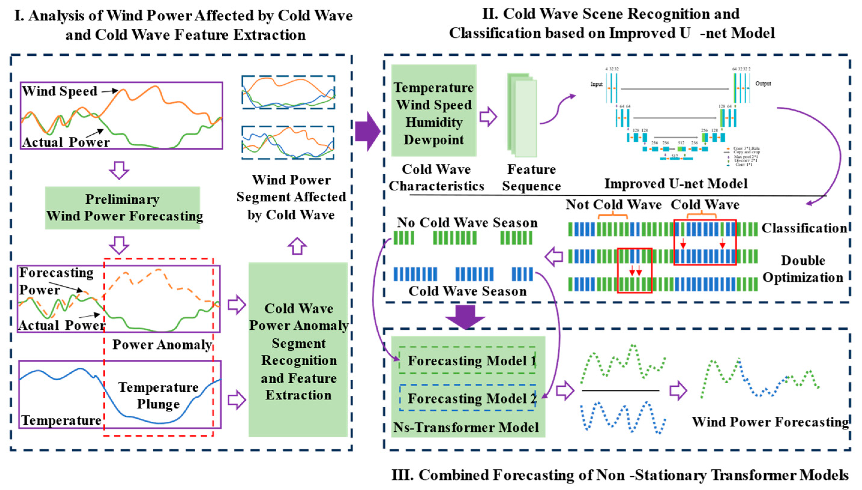
• Proposed cold wave recognition criterion: By considering regional meteorological changes and wind turbine operation characteristics, a cold wave discriminant criterion is proposed. This criterion can accurately identify cold-wave conditions in the region, especially with regard to the duration of the cold wave, providing hour-level accuracy.
• Improved U-Net classification model: Building on the U-Net model, a multi-modal classification method is proposed to optimize the model for the seasonal characteristics of cold waves. The improved model not only accurately forecasts the occurrence time of cold waves but also enhances the recognition accuracy of small-sample cold wave events using cold wave samples generated by an adversarial network.
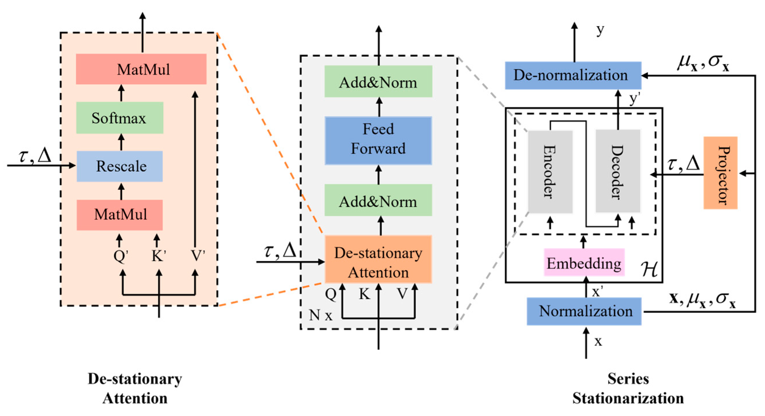
• Construction of wind power combination forecasting model for cold-wave conditions: By combining cold wave recognition results with the Ns-Transformer model, a combined forecasting model for wind power is developed. This model effectively improves the accuracy of day-ahead wind power forecasting during cold conditions and offers a new solution for power forecasting under extreme weather events.

2. Analysis of the Impact of Cold Wave Events on Wind Power Output

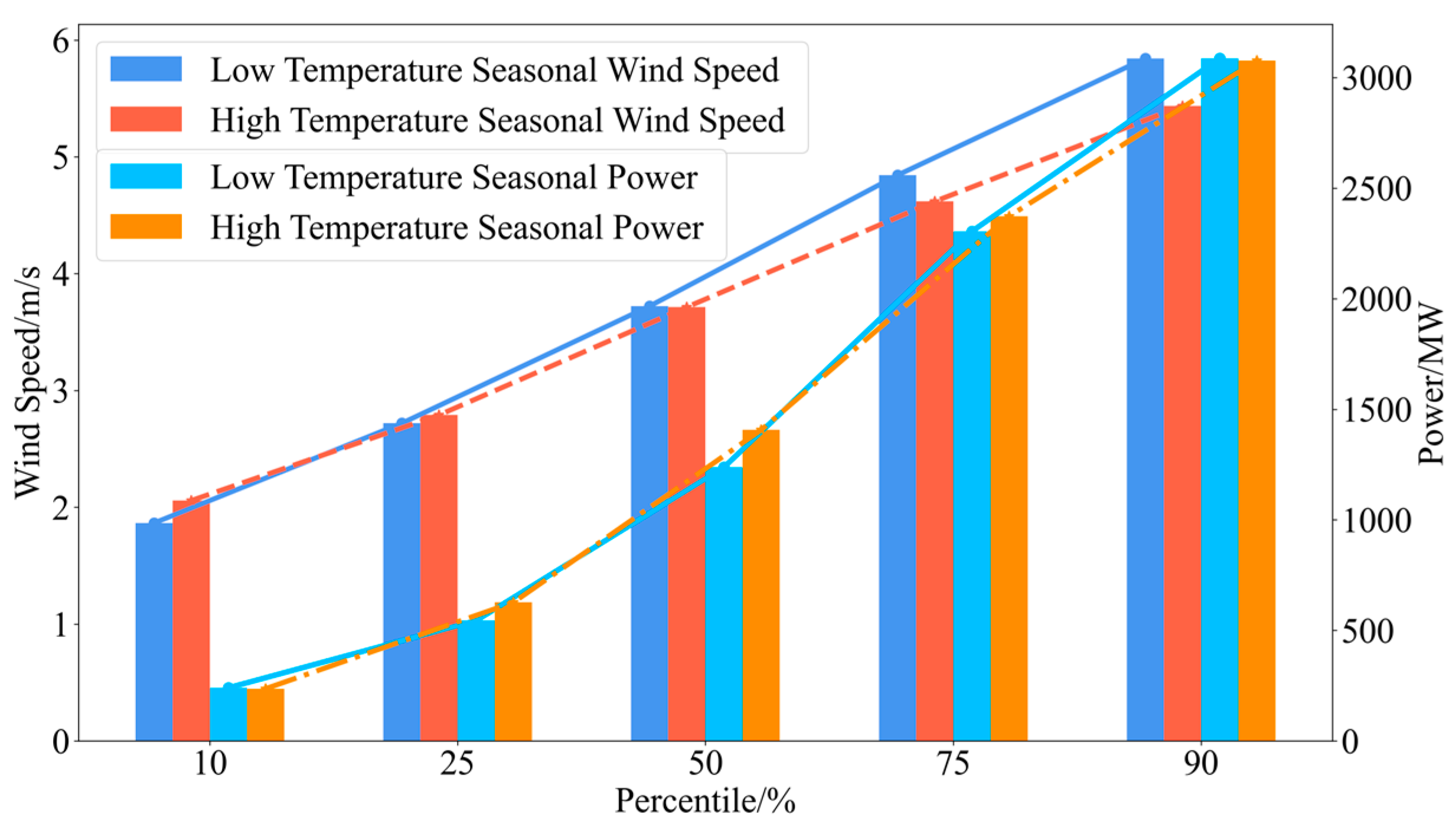
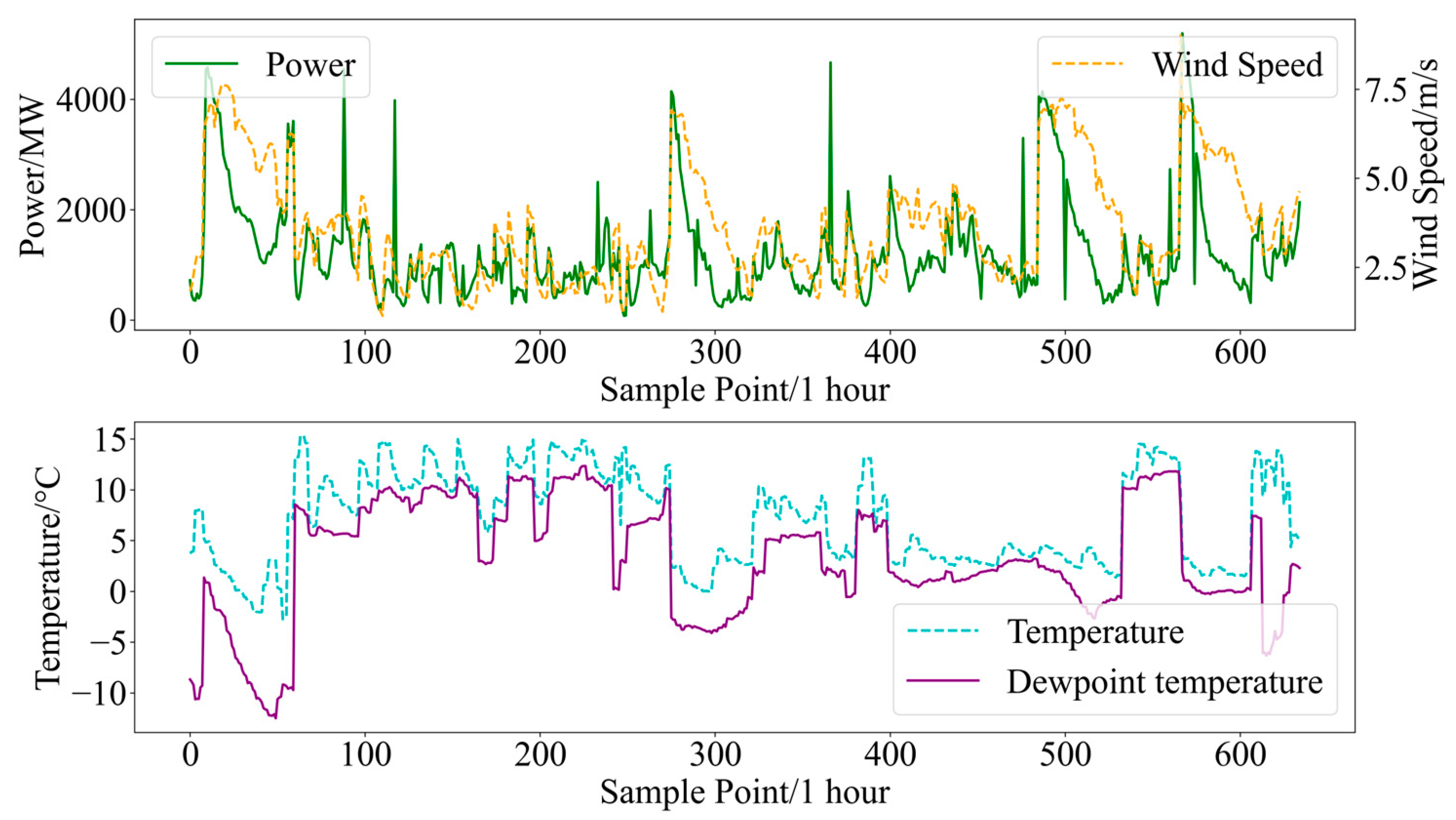
2.1. Influence of Temperature on Wind Power Output

This paper comprehensively analyzes the specific influence of temperature change on wind power output. It calculates the monthly maximum average temperature, average temperature, and minimum average temperature for a certain region over two years, and systematically analyzes the temperature, wind speed, and wind power output data from the past two years, as shown in Figure 2. The bar chart represents the monthly average maximum temperature, average temperature and minimum average temperature, while the curves show the normalized values of the average monthly wind speed and power. The curves represent the normalized values of the average monthly wind speed and power.

The starting wind speed for wind power generation is approximately 3–5 m/s. However, according to the data in Figure 3, around 50% of the wind speeds in the high-temperature season are lower than 3.5 m/s, and most wind speeds do not meet the turbine’s starting wind speed requirements, resulting in low wind turbine output. In the 90th percentile of the wind speed distribution, wind speeds in the high-temperature season are lower than those in the low-temperature season, leading to a lower overall wind speed and, consequently, lower output in the high-temperature season.

Among the various meteorological factors, temperature demonstrates distinct diurnal and seasonal variations that significantly influence wind power output [32]. This study conducts a comprehensive analysis of temperature’s impact on wind power generation. We calculated the monthly maximum average temperature, monthly mean temperature, and monthly minimum average temperature for a specific region over a two-year period. Through systematic analysis of two-year historical data encompassing temperature, wind speed, and wind power output, the relationships are visualized in Figure 2. In this figure, the bar charts depict monthly-averaged maximum, mean, and minimum temperatures, while the dual-axis curves illustrate normalized values of both monthly average wind speed and power output.

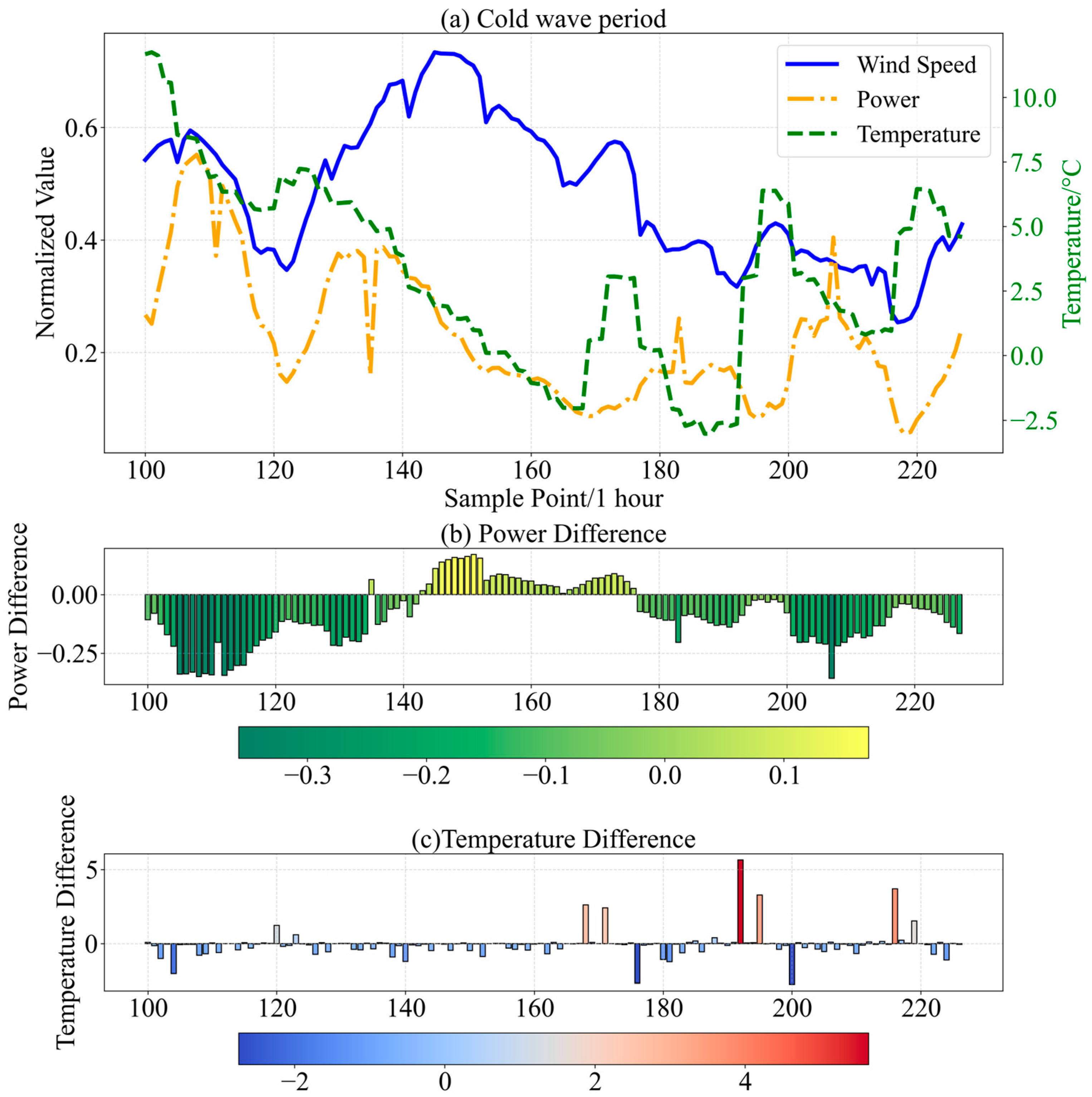
2.2. Influence of Cold Wave Events on Wind Power Output

The relationship between wind generator power and wind speed is given by Equation (1), where wind power is proportional to the cube of wind speed. Therefore, the trends of wind power and the cube of wind speed should be similar. To further analyze this relationship, this study calculates the difference between predicted and actual power after regional normalization and compares the trends of wind speed, temperature, and power during the same period. The specific results are presented in Figure 4.

$$P={\displaystyle \frac{1}{2}}\rho A{v}^3{C}_p$$

(1)

$P$ is the output power of the wind turbine (in watts, W). $\rho$ is the air density, $A$ is the swept area of the wind turbine (in square meters, m²), $A=\pi R^2$, and $R$ is the blade radius of the wind turbine (in meters, m). $Cp$ is the power coefficient, which indicates the efficiency of the wind turbine, with a theoretical maximum value of 0.59, typically lower in practice. $v$ is the wind speed (meters per second, m/s).

Figure 4a presents a comparison of normalized wind speed, temperature, and normalized power. The selected period, from 4 January to 9 January 2021, encompasses a complete cold wave event. The temporal evolution of meteorological parameters is characterized by hourly sampled data points. During this period, the temperature shows a rapid decline, accompanied by an increase in wind speed. However, wind power did not correlate with wind speed and instead followed the trend of temperature. This suggests that during cold wave events, wind power decreases despite the increase in wind speed. Consequently, the correlation between wind power and temperature increases, while the correlation with wind speed decreases during cold wave events.

Figure 4b illustrates the difference between the normalized forecasting and actual power, ranging from −1 to 1. When the difference is greater than 0, it indicates that the wind speed is high, but the output power is low. This observation is consistent with the phenomenon of reduced wind power output during cold wave events, suggesting that cold wave events negatively affect wind power forecasting accuracy. Therefore, the difference between forecasting and actual power can serve as a useful reference index for detecting cold wave events and assessing its impact on wind power output.

Figure 4c displays the first-order difference results for temperature. During cold wave events, the temperature demonstrates a persistent downward trend with consecutive negative differential values. The evolution of cold wave weather is marked by temperature drops and subsequent rises when temperatures return to normal levels, following typical diurnal pattern, indicating the restoration of conventional meteorological conditions.

2.3. Cold Wave Event Criteria

The impact of cold wave events on wind power generation was preliminarily analyzed in the preceding section. While cold wave events are typically associated with a significant temperature decline, wind speed variations exhibit complex patterns, making wind power forecasting based solely on wind speed inherently challenging. During cold wave events, a decrease in wind speed correlates with reduced wind power output, and such predictable variations have a limited impact on forecasting accuracy. However, anomalous scenarios in which wind power output decreases despite increasing wind speeds—likely due to mechanical failures induced by icing—significantly degrade forecasting accuracy. To enable precise assessment of cold event impacts on wind farms, it is imperative to establish multidimensional cold wave event recognition criteria that quantify operational impacts on wind power output.

2.3.1. Cold Wave Event Meteorology Criteria

Based on meteorological principles and the characteristics of wind power, the occurrence of cold weather is typically associated with a sharp drop in temperature. Meteorological standards of cold waves refer to the standards of cold waves issued by China Meteorological Center. This study proposes the following criteria for cold wave events:

A daily minimum temperature below 5 °C, i.e.,

$$T_{\min ,t}\le 5°\mathrm{C}$$

(2)

T_min,t is the minimum temperature of day.

The daily minimum temperature change exceeds 8 °C.

$$\Delta T=T_{\min ,t-1}-T_{\min ,t}\ge 8°\mathrm{C}$$

(3)

T_min,t−1 is the minimum temperature of $t-1$ day.

When Equations (2) and (3) are simultaneously satisfied, day $t$ is classified as a cold wave.

2.3.2. Comprehensive Judgment Conditions Based on Cold Wave Events Judgment and Wind Power Deviation

Building on the cold wave events judgment, the relationship between wind speed and power must also be taken into account. Specifically, when wind speed is high, wind power does not increase proportionally. In this case, wind speed is high, but power is low, leading to diminished wind power forecasting accuracy. Therefore, the following judgment conditions can be proposed.

The difference between the normalized predicted wind power and the actual power exceeds 0.15 of the total installed capacity.

$$\Delta P=\left|\left.P_{pred}^{\prime }-P_{ture}^{\prime }\right|\right.\ge 0.15Cap$$

(4)

$P_{pred}^{\prime }$ represents the predicted data after normalization, $P_{ture}^{\prime }$ represents the actual power data after normalization, and $Cap$ is the total installed capacity of wind farm cluster power.

When both the cold wave event judgment conditions and the difference between the normalized predicted power and actual power exceeding 0.15 of the total installed capacity are observed, it can be concluded that cold wave events significantly impact wind power output at this time.

3. The Method Presented in This Paper

The occurrence of a cold wave significantly impacts the accuracy of wind power forecasting. Therefore, prior to wind power forecasting, it is crucial to assess the likelihood of a cold wave occurring in the next period using NWP data. By inputting cold wave features, the cold wave event is classified, and a cold wave recognition model is established.

3.1. Cold Wave Recognition Process

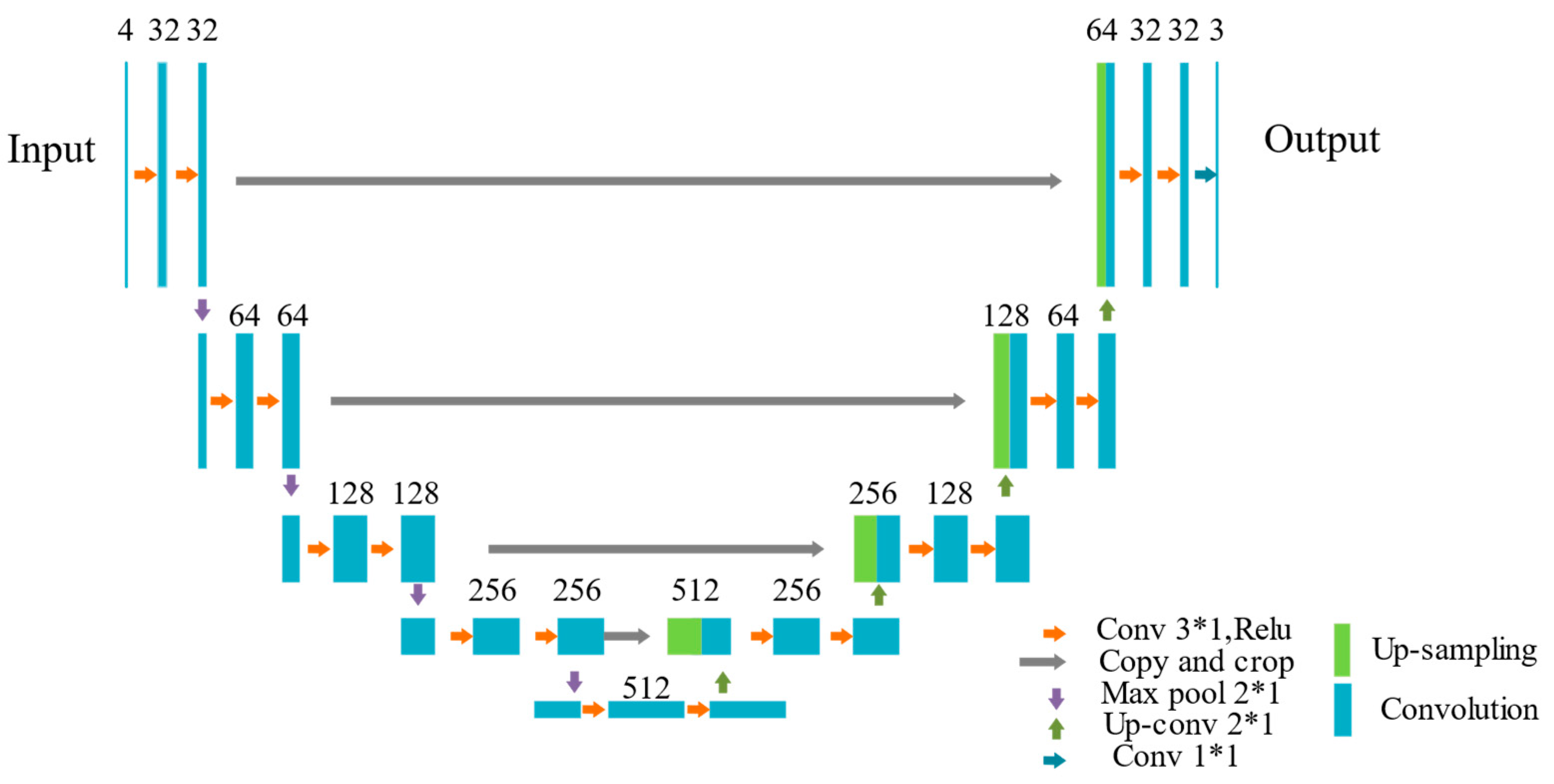
3.1.1. Cold Wave Weather Recognition Model Based on Improved U-Net

The U-Net model is a deep learning architecture designed for data segmentation [37]. It consists of a contracting path on the left and an expansive path on the right, forming a U-shaped structure, hence the name “U-Net.” The specific structure is shown in Figure 5. The contracting path follows a typical CNN structure, consisting of two convolutional layers followed by a max pooling layer. The dimensionality of cold wave features doubles after each pooling operation. The contracting path uses $Relu$ as the activation function.

$$Relu(x)=max\{0,x\}$$

(5)

The input value is $x$. It is compared with 0; if $x$ > 0, the output is $x$, and if $x$ ≤ 0 the output is 0.

In the expansive path, a transposed convolution operation is performed to double the spatial resolution of the cold wave feature data generated by the contracting path. The feature data are then concatenated with the corresponding feature from the contracting path, further increasing the spatial resolution. Two convolutional layers are subsequently applied for feature extraction, and this structure is repeated. The U-Net can learn more features of cold spells from limited data by increasing the dimensionality through convolution and concatenating data features, thus improving the model’s generalization ability to recognize cold spells, making it superior to conventional classification models.

The number of feature channels in the final convolution layer is set to match the number of categories, and the convolution kernel size is set to 1 × 1. The corresponding cold wave feature data are predicted using the cross-entropy loss function. Finally, the $Softmax$ f function is used to obtain the probability distribution, which classifies whether a cold wave occurs based on the input features. The $Softmax$ function is expressed as follows:

$$Softmax(z_i)={\displaystyle \frac{e^{z_i}}{{\displaystyle \sum _{j=1}^K{e}^{z_j}}}}$$

(6)

$z_i$ is the $i\text{-}\mathrm{th}$ element of the input vector, $K$ is the total number of classes, and $e$ is the base of the natural logarithm.

The cross-entropy loss function is defined as follows:

$$E={\displaystyle \sum _{x\in \Omega }\omega }(x)\log (p_{l}x)$$

(7)

where $\omega (x)$ represents the regulation function, $p_{l}x$ represents the recognition label function, and $l=\{1,\cdots ,K\}$ represents the label of each feature.

Fusing different data types to fully leverage multi-dimensional information has become a key strategy for improving model performance. In this paper, a multi-modal U-Net classification model is proposed, which combines time features such as season and month with cold wave feature data in the compressed channel of the model. Cold wave events exhibit distinct seasonal patterns, and incorporating multi-modal data allows the U-Net model to effectively capture temporal information, thus significantly enhancing the accuracy of cold wave event recognition. This method not only strengthens the model’s ability to capture cold wave occurrence patterns but also enhances the accuracy of cold wave recognition. The parameters of the multimodal U-Net classification model are shown in

Table 2. Parameters of the multimodal U-Net classification model.

Layer Type	Input Channels	Output Channels	Kernel Size	Activation	Operation
Input Layer	4	32
Lower Sampling 1	32	64	3 × 1	ReLU	Conv 3 × 1
Lower Sampling 2	64	128	3 × 1	ReLU	Conv 3 × 1
Lower Sampling 3	128	256	3 × 1	ReLU	Conv 3 × 1
Lower Sampling 4	256	512	3 × 1	ReLU	Conv 3 × 1
Upper Sampling 1	256	512	2 × 1	ReLU	Conv 2 × 1
Upper Sampling 2	512	128	2 × 1	ReLU	Conv 2 × 1
Upper Sampling 3	128	64	2 × 1	ReLU	Conv 2 × 1
Upper Sampling 4	64	2	1 × 1	Softmax	Conv 1 × 1
Bottleneck	256	512	3 × 1	ReLU	Conv 3 × 1

.

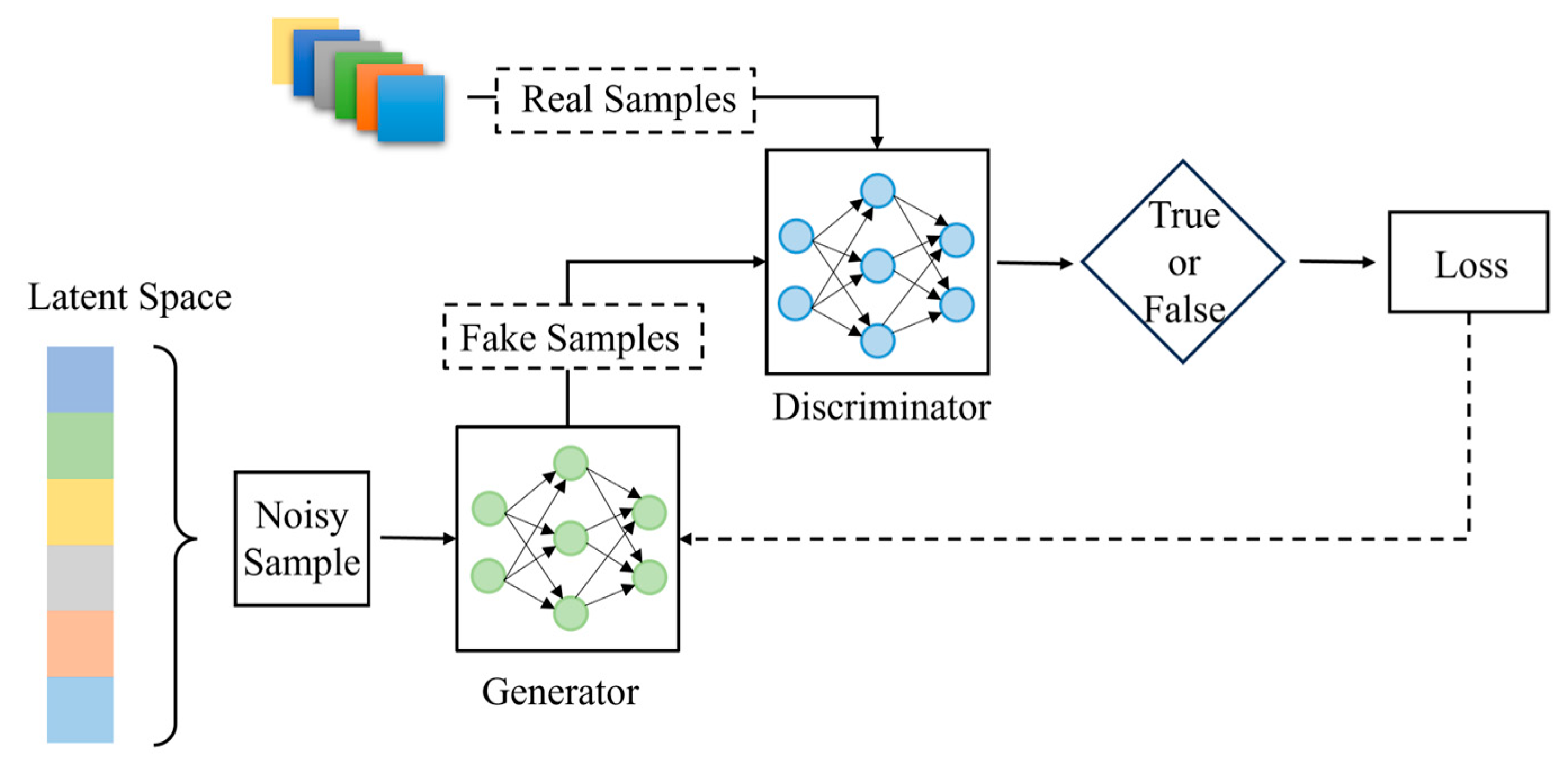
3.1.2. Cold Wave Recognition Under Small Sample Conditions

Imbalanced distribution and insufficient sample size may prevent the classification model from fully learning the sample characteristics during training, leading to the reduced reliability of the forecasting results. This issue is particularly pronounced for small-sample events. Cold wave events are typical examples of small-sample events. To address this issue, this paper uses GANs to generate data samples based on the existing characteristics of cold wave samples.

GANs are deep learning architectures comprising two adversarial neural networks: the Generator and the Discriminator [38]. The structure of the GANs is shown in Figure 6. The generator receives random noise, such as Gaussian or uniform noise, as input, and generates cold wave samples that closely match the real data distribution. Through learning, the generator makes it difficult for the discriminator to distinguish between generated and real samples, thereby continuously improving the quality of the generated data.

As a classification neural network, the discriminator’s goal is to accurately distinguish whether the input data come from real samples or cold wave samples generated by the generator. The generator and discriminator have opposing objectives: the generator aims to maximize the discriminator’s classification error, while the discriminator seeks to minimize the error rate. In this adversarial process, the two networks optimize each other, continuously improving their performance.

Through this adversarial learning process, GANs are capable of generating cold wave samples consistent with the distribution of real data. Ultimately, the generator is able to produce data highly similar to that of real cold wave samples, providing sufficient cold wave sample data for subsequent classification model training and significantly alleviating the issue of insufficient cold wave samples.

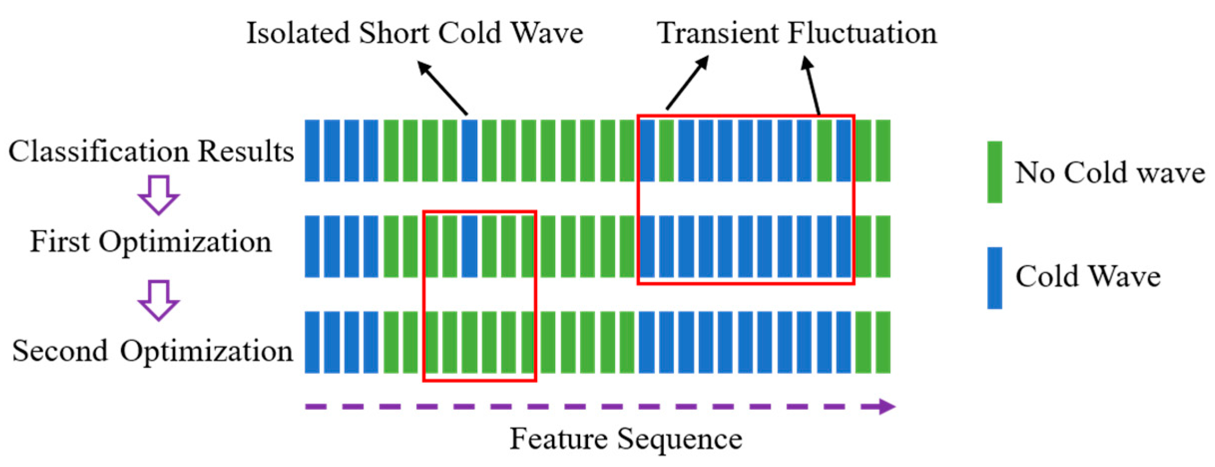
3.1.3. Classification Optimization Approach Based on Continuous Cold Wave Events

The cold wave event process exhibits persistent characteristics, and its impact on wind turbines typically lasts for several hours. For short cold waves with a duration of two hours or less, their occurrence can be categorized into two cases:

• Transient fluctuations within a long cold wave: In the case of a prolonged cold wave, the temperature may temporarily rise, but the wind turbine continues to be affected by the cold wave.
• Isolated short-term cold wave: This refers to a brief cold wave event that appears sporadically in a time series that has not experienced a cold wave for a long period. These short-duration cold waves have a relatively small impact on wind power and can be treated as normal weather conditions.

Given the particularities of short cold wave events, continuous optimization of the cold wave occurrence judgment is necessary to improve the accuracy of future cold wave forecasting. The first optimization step merges short-term fluctuations, which may cause misjudgments, into the ongoing cold wave period. The secondary optimization step combines isolated short-term cold wave events with normal weather, thereby avoiding misclassification and improving the classification results. The specific method for this optimization process is shown in Figure 7.

3.2. Wind Power Forecasting During Cold Wave Events

The Ns-Transformer model is an enhanced version of the Transformer model designed to address the challenges of unstable time series forecasting [39]. This model retains the standard encoder–decoder architecture of the original Transformer used for time series forecasting. To overcome the issue of over-stabilization when directly stabilizing the data, the Non-Stationary Transformer replaces the standard self-attention module with a de-stationary attention module, thereby improving the model’s forecasting performance on non-stationary sequences. The Ns-Transformer model primarily consists of a series stationarization and a de-stabilization attention module. Figure 8 illustrates the structure of the Ns-Transformer model.

$x$ is the input matrix, $x\prime$ is the matrix obtained after the normalization of $x$, and ${\mu }_x,{\sigma }_x$ is the mean and standard deviation of $x$. $\mathcal{H}$ is the module, including the embedding layer, encoder and decoder, $Q$, $K$ and $V$ are three matrices of the same size obtained by smoothing the input characteristic variables, $G$ is the matrix obtained after the $\mathcal{H}$ module, $y$ is the matrix of $y\prime$ after de-normalization, and $\tau ,\Delta$ is the destabilization factor.

Series stationarization primarily consists of the standardization and de-standardization modules. To mitigate the non-stationarity of each input sequence, the temporal dimension is normalized using an $x$ sliding window approach. Each input matrix $x$ is transformed through translation and scaling operations to produce $x\prime$. The expression for the normalization module is as follows:

$${\mu }_x={\displaystyle \frac{1}{k}}{\displaystyle \sum _{c=1}^k{x}_c}$$

(8)

$${\sigma }_x={\displaystyle \frac{1}{k}}{\displaystyle \sum _{c=1}^k{(x_c-{\mu }_x)}^2}$$

(9)

$$x_h\prime ={\displaystyle \frac{1}{\sqrt{{\sigma }_x}}}(x_c-{\mu }_x)$$

(10)

where $k$ represents the total number of samples of $x$, ${\sigma }_x$ is the variance in $x$, $x_c$ is the value of the fixed column in $x$, and $x_h\prime$ is the value of the fixed column in $x\prime$.

After passing through the $\mathcal{H}$ module to obtain $y$, the de-normalization module uses the information of ${\mu }_x$ and ${\sigma }_x$ recorded during normalization to map the model’s output back to $y$, recovering the information lost during normalization. The expression of the de-normalized module is as follows:

$$y\prime =H(x\prime )$$

(11)

$$y={\sigma }_x(y_q\prime +{\mu }_x)$$

(12)

In order to learn attention directly from the time series before stationarity, the disappeared non-stationary information was reintroduced into the calculation of the non-stationary sequence, and the non-stationary factors $\tau$ and $\Delta$ were learned from statistics ${\mu }_x$ and ${\sigma }_x$ of the non-stationary $x$ through the Multilayer Perceptron module. The non-stationary attention module can enhance the predictability of the stationary sequence while preserving the inherent time dependencies of the original sequence, as expressed below.

$$M(Q,K,V,\tau ,\Delta )=Softmax({\displaystyle \frac{\tau Q{K}^{\mathrm{T}}+{\Delta }^{\mathrm{T}}}{\sqrt{e}}})V$$

(13)

$M$ is the attention function; $e$ is the input dimension.

The Softmax function operates on the scaled attention score matrix to generate a normalized attention weight matrix. Each row of this weight matrix corresponds to a query position, with element values constrained within the interval (0,1) and normalized to sum to unity across each row. This probabilistic formulation enables the weighted aggregation of the value matrix V, dynamically capturing long-range dependencies within the sequence while establishing a rigorous probabilistic foundation for subsequent feature integration.

4. Case Study

4.1. Data Presentation and Analysis

4.1.1. Data Presentation and Evaluation Metrics

A wind farm cluster in Jiangxi Province of China consists of 67 wind farms, with a total installed capacity of 5388.9 MW. The wind farms are distributed within the latitude range of 24° N to 30° N and the longitude range of 113° E to 118° E. The data span from 1 January 2021, to 30 December 2022, and include measured power, as well as NWP data for 100 m wind speed, 10 m wind speed, temperature, dew point temperature, and other relevant variables. All data were sampled at an interval of one hour. The power measurements are aggregated.

Figure 9 shows the distribution of the duration and frequency of cold waves in a certain area over two years. The duration of most cold waves is concentrated between 1 and 10 h, and cold wave events lasting more than 30 h are rare. However, cold waves with longer durations can have a significant impact on the operation of wind turbines, particularly under extreme weather conditions, where turbine equipment may suffer from icing and unstable power output. These effects not only reduce the operational efficiency of wind turbines but also lead to a considerable decrease in the accuracy of wind power forecasts, which, in turn, affects grid scheduling and the stability of the energy supply. Therefore, accurately identifying cold waves and predicting their impact on wind farms is crucial for improving the accuracy of wind power forecasting and ensuring the safety of power systems.

Based on the analysis of cold wave judgment criteria, cold wave events are primarily influenced by temperature and wind speed. Figure 10 presents the curves of power, wind speed, temperature, and dew point temperature during all cold wave periods.

Cold wave event recognition is performed using the improved U-Net model, Random Forest, K-Nearest Neighbors (KNNs), Multilayer Perceptron (MLP), Support Vector Machine (SVM), and Long Short-Term Memory (LSTM) models to classify the data. The dataset consists of 17,520 samples, with an 8:2 split between the training and test sets. Among the six classification models, accuracy, precision, recall, and the F1 score are used to evaluate the classification performance.

$$Accuracy={\displaystyle \frac{TP+TN}{TP+TN+FP+FN}}$$

(14)

$$Precision={\displaystyle \frac{TP}{TP+FP}}$$

(15)

$$Recall={\displaystyle \frac{TP}{TP+FN}}$$

(16)

$$F_1=2\times {\displaystyle \frac{Accuracy\times Precision}{Accuracy+Precision}}$$

(17)

where $TP$ represents the number of samples correctly predicted as positive, $TN$ represents the number of samples correctly predicted as negative, $FP$ represents the number of samples incorrectly predicted as positive, and $FN$ represents the number of samples incorrectly predicted as negative.

The time scale for wind power forecasting is day-ahead forecasting. The forecasting method used is a combined approach, as cold wave events exhibit clear seasonality, primarily occurring in January, February, November, and December. Therefore, the data are divided into periods with cold wave occurrences and periods without cold wave occurrences. The division of the training and test sets is shown in

Table 3. Forecasting data split training set and test set.

Type	Training Set	Test Set
Cold wave occurs	January–February, November–December 2021	November–December 2022
No Cold wave occurs	March–October 2021	September–October 2022

.

In this paper, the Mean Absolute Error (MAE) and Root Mean Square Error (RMSE) are used to evaluate the forecasting results. The calculation formulas are as follows:

$$N_{MAE}={\displaystyle \frac{1}{n}}\cdot {\displaystyle \sum _{i=1}^n\frac{\left(P_i-{\widehat{P}}_i\right)}{Cap}}$$

(18)

$$N_{RMSE}={\displaystyle \frac{1}{Cap}}\sqrt{{\displaystyle \frac{1}{n}}\cdot {\displaystyle \sum _{i=1}^n{\left(P_i-{\widehat{P}}_i\right)}^2}}$$

(19)

$P_i$ represents the actual value, ${\widehat{P}}_i$ is the predicted value, and $Cap$ is the rated installed capacity of the wind farm.

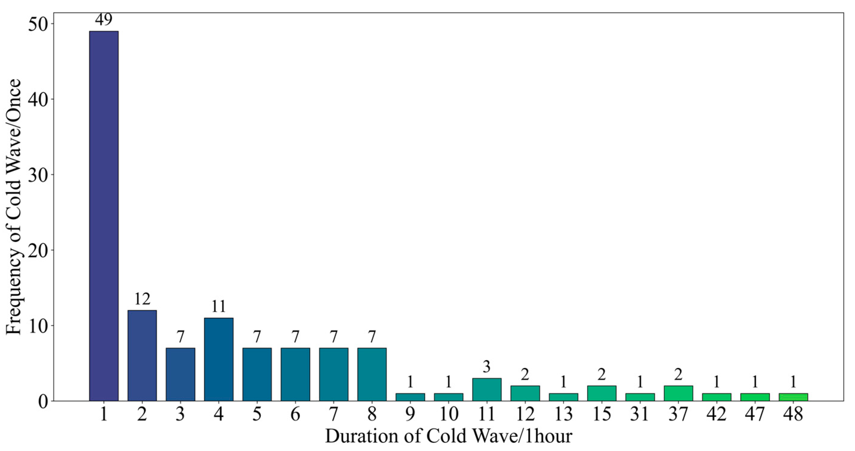
4.1.2. Analysis of Cold Wave Weather Characteristics

Through the analysis of the relevant data over the two-year period, it was determined that during the 730 days of the observation period, cold waves occurred for a total of 681 h, accounting for approximately 3.89% of the total duration. The distribution of the duration and frequency of cold waves is shown in Figure 9.

The duration of most cold waves is concentrated between 1 and 10 h, and cold wave events lasting more than 30 h are rare. However, cold waves with longer durations can have a significant impact on the operation of wind turbines, particularly under extreme weather conditions, where turbine equipment may suffer from icing and unstable power output. These effects not only reduce the operational efficiency of wind turbines but also lead to a considerable decrease in the accuracy of wind power forecasts, which, in turn, affects grid scheduling and the stability of the energy supply. Therefore, accurately identifying cold waves and predicting their impact on wind farms is crucial for improving the accuracy of wind power forecasting and ensuring the safety of power systems.

Based on the analysis of cold wave judgment criteria, cold wave events are primarily influenced by temperature and wind speed. Figure 10 presents the curves of power, wind speed, temperature, and dew point temperature during all cold wave periods.

In order to further investigate the key factors influencing the occurrence of cold waves, this paper performs Pearson correlation coefficient analysis on the relevant meteorological data during cold waves, aiming to reveal the relationship between meteorological variables and wind power during these events. The Pearson correlation coefficient formula is shown in Equation (20).

$$r={\displaystyle \frac{n{\displaystyle \sum x_i}{y}_i-{\displaystyle \sum x_i}{\displaystyle \sum y_i}}{\sqrt{\left(n{\displaystyle \sum x_i^2}-{({\displaystyle \sum x_i})}^2\right)\left(n{\displaystyle \sum y_i^2}-{({\displaystyle \sum y_i})}^2\right)}}}$$

(20)

$r$ is the Pearson correlation coefficient, $n$ is the number of data points, $x_i$ is the $x$ value for the $i$ th sample, and $y_i$ is the $y$ value for the $i$ th sample.

Temperature 1 represents the hourly temperature, while temperature 2 refers to the dew point temperature. Difference 1 denotes the hourly temperature difference, and difference 2 refers to the daily minimum temperature difference. According to the analysis results presented in Figure 11, the correlation between power and the 100 m wind speed, 10 m wind speed, daily minimum temperature difference, and hourly temperature difference is highest during cold wave events.

4.2. Recognition Result

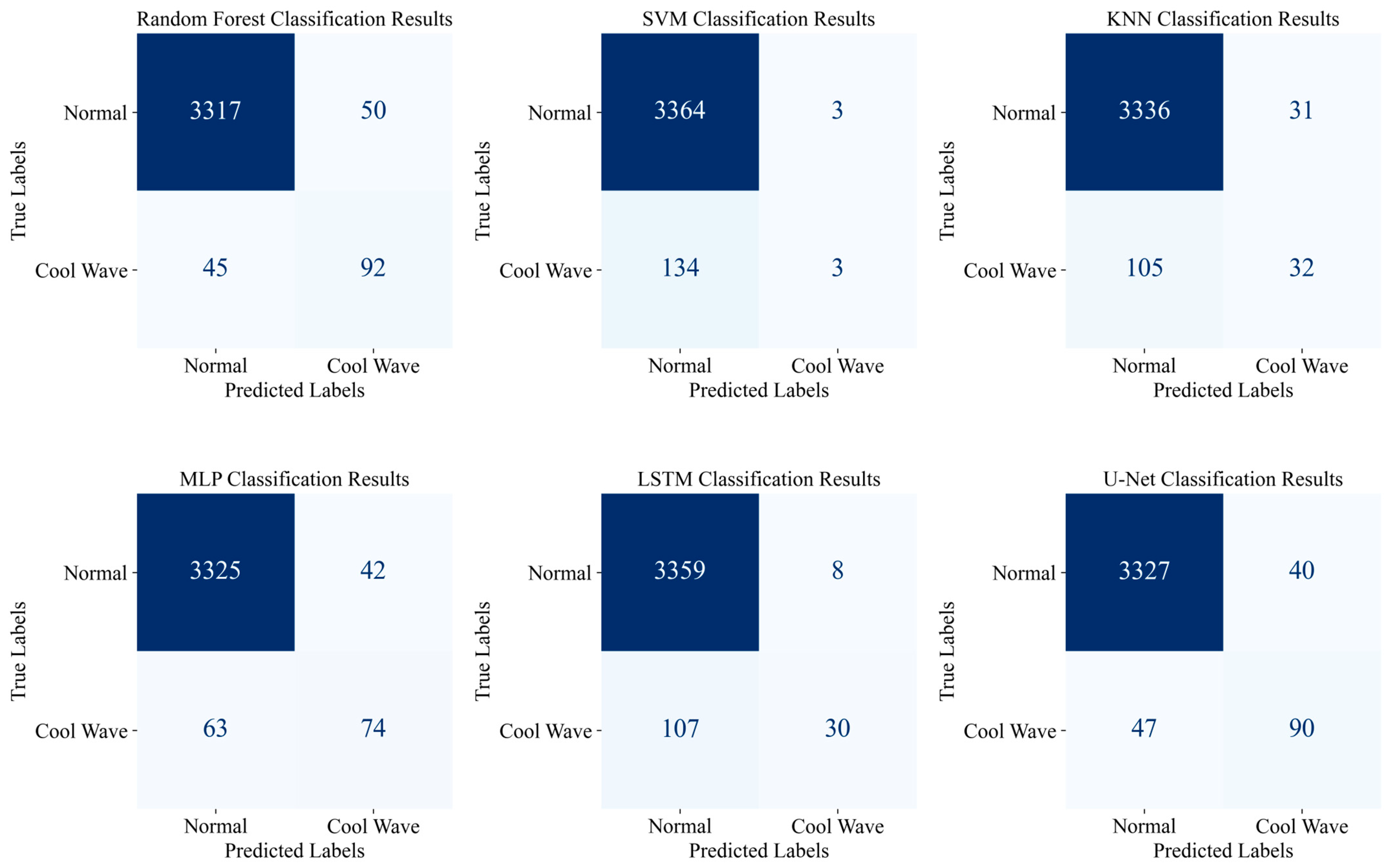
4.2.1. Cold Wave Weather Identification Under Small Sample Conditions

The results of each classification model are presented in Figure 12 as heat maps, which allow for an intuitive comparison of the classification performance. It can be seen that the recognition accuracy of all six classification models is generally high. The improved U-Net model proposed in this paper achieves the highest classification accuracy, followed by the random forest model and the LSTM model. However, while each classification model demonstrates high accuracy in recognizing non-cold wave events, there are significant differences in recognizing cold wave events. The individual recognition recall rates for cold wave events in the improved U-Net model, random forest model, and LSTM model are 0.667, 0.671, and 0.540, respectively, as shown in

Table 4. Evaluation of classification results for different classification models.

Model	Accuracy	Precision	Recall	F1
Random Forest	0.9729	0.9734	0.6175	0.9731
SVM	0.9609	0.9436	0.0219	0.9434
KNN	0.9612	0.9514	0.2336	0.9542
MLP	0.9672	0.9611	0.5401	0.9620
LSTM	0.9706	0.9665	0.2189	0.9674
U-Net	0.9775	0.9789	0.6569	0.9780

.

As small-sample events, cold wave events accounts for only 3.8% of the total data over two years. This sample imbalance significantly affects the training process and classification performance of the model, particularly in the classification of cold wave event data. The lack of cold wave samples can lead to high overall classification accuracy. The number of cold wave samples in the test set is 137, and the recall rates for cold wave samples, as calculated by different models, are shown in Table 4. The recall rate reflects the model’s ability to correctly identify real cold wave events.

As shown in Table 4, the SVM model demonstrates extremely low recognition ability for cold wave weather, primarily due to the scarcity of cold wave samples, which prevents the model from fully learning the cold wave features during training.

While all classification models exhibit relatively high accuracy, this elevated accuracy may lack practical significance. Due to the scarcity of cold wave samples, the models tend to misclassify cold wave events as normal weather. However, given the limited number of cold wave instances in the dataset, their misclassification has a minimal impact on the overall accuracy metric. Consequently, relying solely on accuracy metrics fails to reflect the model’s true capability in effectively identifying real-world cold wave events. This result underscores the importance of feature enhancement and data augmentation for small-sample cold wave data and provides a research direction for improving model performance under imbalanced data conditions.

4.2.2. Cold Wave Weather Recognition Under GAN Sample Generation

After using GANs to generate 5000 cold wave samples and mixing these generated samples with the original training data, the total number of samples in the training set was expanded to 22,520. At the same time, the test set remains composed of original data, with 3504 samples. In this experiment, different classification models were used to train the augmented training set, and their classification performance was evaluated on the test set. The results are presented in

Table 5. Evaluation of classification results of generated data.

Model	Accuracy	Precision	Recall	F1
Random Forest	0.9863	0.8069	0.8540	0.8300
SVM	0.9823	0.8100	0.7153	0.7600
KNN	0.9899	0.8500	0.9051	0.8700
MLP	0.9926	0.8936	0.9198	0.9000
LSTM	0.9951	0.9412	0.9344	0.9300
U-Net	0.9971	0.9568	0.9731	0.9600

. Through the generation and expansion of cold wave samples, the number of cold wave samples in the training set was significantly increased. Experimental results demonstrate that this method improves the recall rates of all six classification models to varying degrees. Among these models, the recall rate of the SVM model showed a notable improvement, rising to 0.7153, indicating that the recognition ability of the SVM model for real cold wave data has been substantially enhanced under this data augmentation approach.

Using data generation techniques to augment cold wave samples not only enhances the classification model’s ability to learn cold wave features but also significantly improves its recognition of cold wave events. This method effectively mitigates the classification bias caused by sample imbalance and reduces the poor recognition performance for some data categories due to insufficient samples. Overall, the data augmentation strategy, assisted by GANs, provides a practical solution for improving the performance of classification models in the context of small sample sizes and imbalanced data.

4.3. Wind Power Forecasting Results

4.3.1. Comparison of Power Forecasting Results of Different Models

In this study, LSTM, BP, Random Forest, Transformer, and Ns-Transformer are used for wind power forecasting, with separate training and forecasting for data from the cold-wave and non-cold-wave seasons. The evaluation metrics for the forecasting results are presented in

Table 6. Evaluation metrics for the prediction results of different models.

	Cold Wave Season		Non-Cold Wave Season
Model	RMSE	MAE	RMSE	MAE
LSTM	0.1642	0.1144	0.1244	0.0935
Random Forest	0.1635	0.1189	0.1302	0.1042
BP	0.1558	0.1100	0.1579	0.1229
Transformer	0.1121	0.0854	0.0881	0.0785
Proposed Method	0.1077	0.0849	0.0842	0.0692

. In the non-cold-wave season, the Ns-Transformer model proposed in this paper achieves reductions of 3.82%, 4.60%, 7.37%, and 0.39% in RMSE compared to the LSTM, BP, Random Forest, and Transformer models. During the non-cold-wave season, due to relatively small weather fluctuations, both the Transformer and Ns-Transformer models effectively predict the power change trend based on the input features. The forecasting results of the five models during the cold-wave-free season are shown in Figure 13, where the differences in model performance can be visually observed.

However, for the forecasting results in the cold wave season, the performance of the LSTM, Random Forest, Transformer, and the proposed model decreases. The RMSE in the cold wave season is 3.98%, 3.33%, 2.40%, and 2.35% higher than that in the non-cold-wave season, respectively. The occurrence of cold wave events not only brings drastic fluctuations to wind power but also reduces the correlation between wind speed and other factors, thereby decreasing forecasting accuracy. Through comparative analysis, it is evident that the proposed method maintains good forecasting accuracy under cold-wave conditions, with its RMSE increase being significantly lower than that of other methods, making it more suitable for wind power forecasting during cold wave events. In the cold wave season, LSTM, BP, and Random Forest models fail to accurately capture power changes during cold wave events, leading to forecasting power values that are generally higher than the actual power during the cold wave. The cold wave period marked in Figure 14 shows the forecasting of different models for the cold wave. In contrast, the Transformer model achieves better forecasting accuracy for relatively stable power changes but cannot identify the fluctuation trend during severe wind power fluctuations in cold wave events. The Ns-Transformer model, which introduces de-stationary attention based on the Transformer, provides excellent forecasting results even under large fluctuations in wind power.

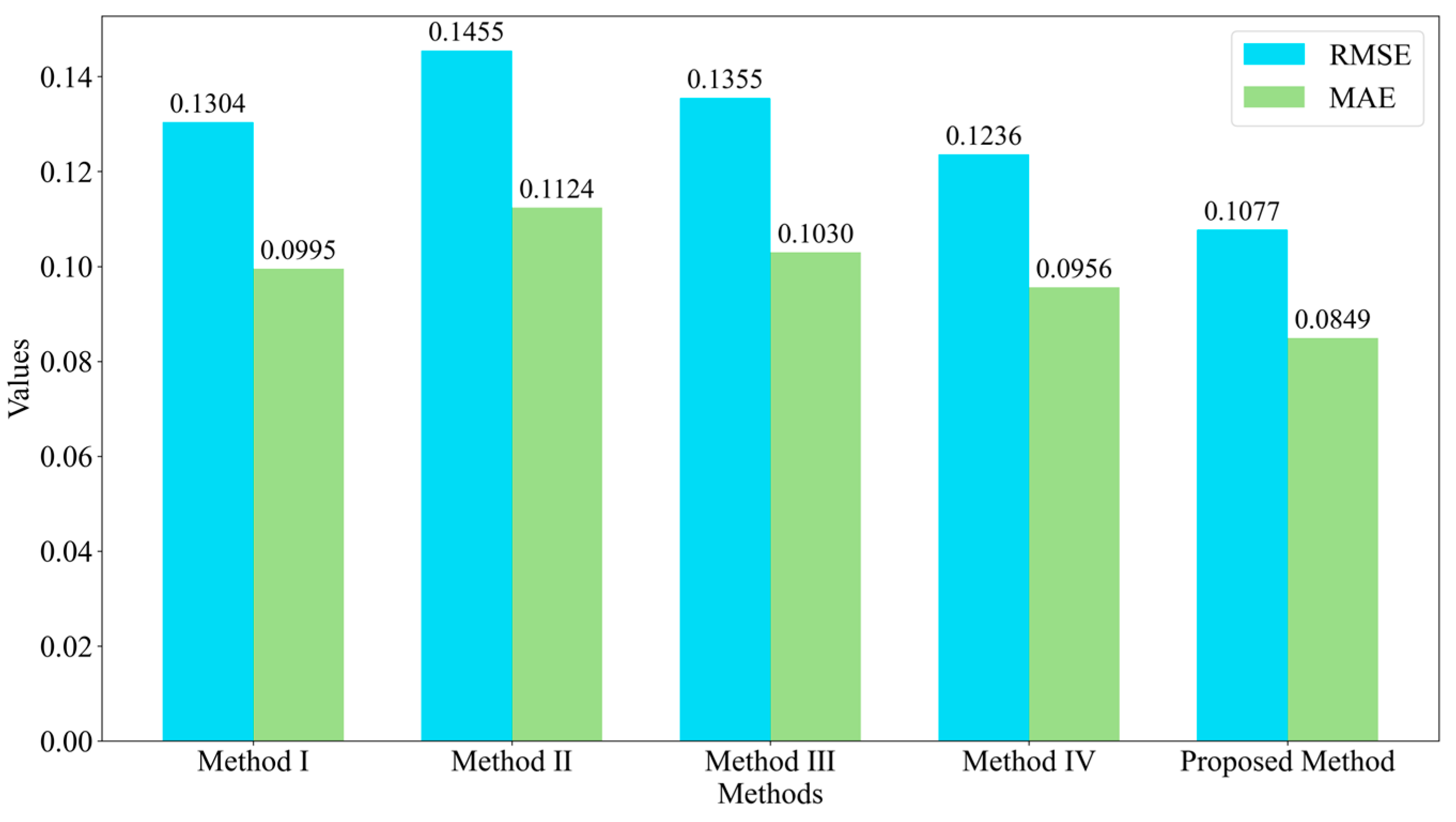
4.3.2. Ablation Experiments for the Forecasting Method

To verify the applicability of the proposed method for seasonal wind power forecasting during cold waves, this paper compares and analyzes wind power forecasting performance of Methods I to IV. The specific details of each forecasting method are shown in

Table 7. Content of various methods for ablation experiments.

Method	Model	Cold Wave Characteristics	Data Generation	Continuity Correction
Method I	Transformer	✓	✓	✓
Method II	Ns-Transformer
Method III		✓
Method IV		✓	✓
Proposed Method		✓	✓	✓

, and the corresponding forecasting results are presented in Figure 15. The RMSE and MAE for the forecasting results are shown in Figure 16. The experimental results indicate that the RMSE and MAE of Methods II to IV and of the proposed method decrease progressively, suggesting that incorporating the cold wave recognition results generated by continuous samples as inputs to the forecasting model can significantly improve the accuracy of wind power forecasting under cold wave events conditions. Compared with those of Method I, the RMSE and MAE of the proposed method are reduced by 2.27% and 1.46%, respectively. Under cold wave conditions with significant wind power fluctuations, the performance of the forecasting model has a substantial impact on the forecasting results. The experimental findings demonstrate that the proposed method outperforms others in wind power forecasting under cold wave events, offering higher forecasting accuracy and applicability.

5. Discussion

To improve the accuracy of cold wave event recognition and enhance wind power forecasting under cold-wave conditions, this paper proposes a recognition method for cold wave events and a day-ahead wind power forecasting model for wind farm clusters.

• Starting with the impact of cold wave weather on wind power, this paper establishes the discriminant criteria for cold wave events and extracts key features through an in-depth analysis of historical data, providing a basis for subsequent cold wave events recognition.
• Aiming to address the recognition problem of small-sample cold wave events, an improved multi-modal U-Net classification model is proposed. Cold wave events samples generated by this model are added to the training set, significantly enhancing the classification model’s ability to recognize cold wave events. The model utilizes future NWP to accurately forecast the occurrence of cold waves, providing an effective early warning for the power system to handle extreme weather events.
• Based on cold wave recognition, this paper establishes distinct wind power forecasting models for the cold-wave and non-cold-wave seasons, respectively. Compared with the experimental results of different classification models, the Ns-Transformer model demonstrates superior wind power forecasting accuracy under cold-wave conditions.

The proposed method emphasizes the consideration of wind power forecasting under cold wave conditions. To further improve the accuracy of wind power forecasting under extreme weather, future work should consider additional extreme weather events, such as strong winds and heavy snow.

6. Conclusions

The proposed method in this study focuses on enhancing wind power prediction accuracy under extreme cold-wave conditions. For cold wave scenario identification, a refined cold wave identification criterion is developed by incorporating the operational characteristics of wind turbines under extreme weather, which reduces the scenario recognition time to an hourly level compared with the criteria in [36]. Considering the limited sample size of cold wave events that may compromise classification accuracy, existing studies [26,27,28] address this issue through sample generation techniques. However, the concurrent inclusion of generated samples in both training and test sets introduces potential evaluation biases. To mitigate this, the proposed method exclusively integrates generated samples into the training set. While current research has achieved cold wave scenario recognition through meteorological pattern classification and weather evolution analysis [23,24,25], insufficient attention has been paid to integrating cold wave forecasting into wind power prediction frameworks. This study bridges this gap by synergizing cold wave identification with wind power prediction, thereby improving forecasting performance under cold-wave conditions.

The developed methodology is particularly applicable to wind farms in cold wave-affected regions where extreme low temperatures significantly influence power generation. Limitations include the following: (1) the current framework exclusively addresses cold wave impacts without considering other extreme weather scenarios (gales or blizzards); (2) the proposed cold wave criterion, optimized for regional weather patterns in the study area, requires parameter adjustments when applied to geographically distinct regions; (3) although sample generation enhancement constitutes a key contribution, the academic community has yet to establish robust evaluation criteria for determining the substitutability of generated samples for original data. Future research should prioritize developing standardized methods for synthetic sample feasibility assessment.

References

1. Yang, M.; Wang, D.; Zhang, W.; Yv, X. A centralized power prediction method for large-scale wind power clusters based on dynamic graph neural network. Energy 2024, 310, 133210. [Google Scholar] [CrossRef]
2. National Energy Administration. 2024 National Power Industry Statistics; National Energy Administration: Beijing, China, 2024. [Google Scholar]
3. Xue, Y.; Lei, X.; Xue, F.; Yu, C.; Dong, Z.; Wen, F.; Ju, P. A Review on Impacts of Wind Power Uncertainties on Power Systems. Proc. CSEE 2014, 34, 5029–5040. [Google Scholar] [CrossRef]
4. Serrano-Notivoli, R.; Lemus-Canovas, M.; Barrao, S.; Sarricolea, P.; Meseguer-Ruiz, O.; Tejedor, E. Heat and Cold Waves in Mainland Spain: Origins, Characteristics, and Trends. Weather Clim. Extrem. 2022, 37, 100471. [Google Scholar] [CrossRef]
5. Zhao, H.; Lin, S.; Qu, Y.; Yang, A.; Chang, J. Reliability Evaluation of Wind Turbine Competitive Failure Considering Extreme Weather Impact Process. Electr. Power Autom. Equip. 2024, 44, 40–47. [Google Scholar]
6. Perera, A.T.D.; Nik, V.M.; Chen, D.; Scartezzini, J.; Hong, T. Quantifying the Impacts of Climate Change and Extreme Climate Events on Energy Systems. Nat. Energy 2020, 5, 150–159. [Google Scholar] [CrossRef]
7. Hang, G.; Zhong, H.; Tan, Z.; Cheng, T.; Xia, Q.; Kang, C. Texas Electric Power Crisis of 2021 Warns of a New Blackout Mechanism. CSEE J. Power Energy Syst. 2022, 8, 1–9. [Google Scholar]
8. Yu, G.Z.; Liu, L.; Tang, B.; Wang, S.Y.; Chung, C.Y. Ultra-Short-Term Wind Power Subsection Forecasting Method Based on Extreme Weather. IEEE Trans. Power Syst. 2023, 38, 5045–5056. [Google Scholar] [CrossRef]
9. Yang, M.; Huang, Y.; Xu, C.; Liu, C.; Dai, B. Review of Several Key Processes in Wind Power Forecasting: Mathematical Formulations, Scientific Problems, and Logical Relations. Appl. Energy 2025, 377, 124361. [Google Scholar] [CrossRef]
10. Zhu, Q.; Li, J.; Qiao, J.; Shi, M.; Wang, C. Application and Prospect of Artificial Intelligence Technology in Renewable Energy Forecasting. Proc. CSEE 2023, 43, 3027–3048. [Google Scholar] [CrossRef]
11. Yang, M.; Li, X.; Fan, F.; Wang, B.; Su, X.; Ma, C. Two-stage day-ahead multi-step prediction of wind power considering time-series information interaction. Energy 2024, 312, 133580. [Google Scholar] [CrossRef]
12. Wang, Y.; Pei, L.; Li, W.; Zhao, Y.; Shan, Y. Short-term wind power prediction method based on multivariate signal decomposition and RIME optimization algorithm. Expert Syst. Appl. 2025, 259, 125376. [Google Scholar] [CrossRef]
13. Yang, M.; Guo, Y.; Wang, B.; Wang, Z.; Chai, R. A Day-ahead Wind Speed Correction Method: Enhancing Wind Speed Forecasting Accuracy Using a Strategy Combining Dynamic Feature Weighting with Multi-Source Information and Dynamic Matching with Improved Similarity Function. Expert Syst. Appl. 2025, 263, 125724. [Google Scholar] [CrossRef]
14. Saoud, L.S.; Al-Marzouqi, H.; Deriche, M. Wind Speed Forecasting Using the Stationary Wavelet Transform and Quaternion Adaptive-gradient Methods. IEEE Access 2021, 9, 127356–127367. [Google Scholar] [CrossRef]
15. Zou, F.; Fu, W.; Fang, P.; Xiong, D.; Wang, R. A Hybrid Model Based on Multi-Stage Principal Component Extraction, GRU Network, and KELM For Multi-Step Short-Term Wind Speed Forecasting. IEEE Access 2020, 8, 222931–222943. [Google Scholar] [CrossRef]
16. Shahid, F.; Zameer, A.; Muneeb, M. A Novel Genetic LSTM Model for Wind Power Forecast. Energy 2021, 223, 120069. [Google Scholar] [CrossRef]
17. Viet, D.T.; Phuong, V.V.; Duong, M.Q.; Tran, Q.T. Models for Short-Term Wind Power Forecasting Based on Improved Artificial Neural Network Using Particle Swarm Optimization and Genetic Algorithms. Energies 2020, 13, 2873. [Google Scholar] [CrossRef]
18. Peng, X.; Wang, H.; Lang, J. EALSTM-QR: Interval Wind-power Prediction Model Based on Numerical Weather Prediction and Deep Learning. Energy 2021, 220, 119692. [Google Scholar] [CrossRef]
19. Chang, Y.; Yang, H.; Chen, Y.; Zhou, M.; Yang, H.; Wang, Y.; Zhang, Y. A Hybrid Model for Long-term Wind Power Forecasting Utilizing NWP Subsequence Correction and Multi-Scale Deep Learning Regression Methods. IEEE Trans. Sustain. Energy 2023, 15, 263–275. [Google Scholar] [CrossRef]
20. Yang, M.; Guo, Y.; Huang, Y. Wind Power Ultra-short-term Forecasting Method Based on NWP Wind Speed Correction and Double Clustering Division of Transitional Weather Process. Energy 2023, 282, 128947. [Google Scholar] [CrossRef]
21. Yu, G.; Lu, L.; Tang, B.; Wang, S.; Dong, Q. Research on Ultra-short-term Subsection Forecasting Method of Offshore Wind Power Considering Transitional Weather. Proc. CSEE 2022, 42, 4859–4871. [Google Scholar] [CrossRef]
22. Sideratos, G.; Hatziargyriou, N.D. Wind Power Forecasting Focused on Extreme Power System Events. IEEE Trans. Sustain. Energy 2012, 3, 445–454. [Google Scholar] [CrossRef]
23. Zhang, J.; Fu, H. An Integrated Modeling Strategy for Wind Power Forecasting Based on Dynamic Meteorological Visualization. IEEE Access 2024, 12, 69423–69433. [Google Scholar] [CrossRef]
24. Lu, X.; Dong, C.; Wang, Z.; Jiang, J.; Wang, B.; Li, B. Research on Short-term Wind Power Forecasting Technology Under Low Temperature and Cold Wave Weather. Power Syst. Technol. 2024, 48, 4833–4843. [Google Scholar] [CrossRef]
25. Ye, L.; Li, Y.; Pei, M.; Li, Z.; Xu, X.J.; Lu, J. Combined Approach for Short-term Wind Power Forecasting Under Cold Weather With Small Sample. Proc. CSEE 2023, 43, 543–555. [Google Scholar] [CrossRef]
26. Fujimoto, Y.; Takahashi, Y.; Hayashi, Y. Alerting to Rare Large-scale Ramp Events in Wind Power Generation. IEEE Trans. Sustain. Energy 2019, 10, 55–65. [Google Scholar] [CrossRef]
27. Yang, M.; Guo, Y.; Huang, T.; Zhang, W. Power Forecasting Considering NWP Wind Speed Error Tolerability: A Strategy to Improve the Accuracy of Short-term Wind Power Forecasting Under Wind Speed Offset Scenarios. Appl. Energy 2025, 377, 124720. [Google Scholar] [CrossRef]
28. Wei, Z.; Liu, Y.; Shen, X.; Liu, J. Ultra-short-term Power Generation Modeling and Prediction for Small Hydropower in Data-scarce Areas Based on Sample Data Transfer Learning. Proc. CSEE 2022, 43, 1–17. [Google Scholar]
29. Peng, X.; Yang, Z.; Li, Y.; Wang, B.; Che, J. Short-Term Wind Power Forecasting Based on Stacked Denoised Auto-encoder Deep Learning and Multi-evel Transfer Learning. Wind Energy 2023, 26, 1066–1081. [Google Scholar] [CrossRef]
30. Chen, H.; Birkelund, Y.; Zhang, Q. Data-augmented Sequential Deep Learning for Wind Power Forecasting. Energy Convers. Manag. 2021, 248, 114790. [Google Scholar] [CrossRef]
31. Liu, Y.; Wang, J.; Liu, L. Physics-informed Reinforcement Learning for Probabilistic Wind Power Forecasting Under Extreme Events. Appl. Energy 2024, 376, 124068. [Google Scholar] [CrossRef]
32. Yang, M.; Guo, Y.; Fan, F. Ultra-short-term prediction of wind farm cluster power based on embedded graph structure learning with spatiotemporal information gain. IEEE Trans. Sustain. Energy 2025, 16, 308–322. [Google Scholar] [CrossRef]
33. Feng, M.; Qin, Y.; Lu, C. An Objective Recognition Method for Wintertime Cold Fronts in Eurasia. Adv. Atmos. Sci. 2021, 38, 1695–1705. [Google Scholar] [CrossRef]
34. Grochowicz, A.; van Greevenbroek, K.; Bloomfield, H. Using power system modelling outputs to identify weather-induced extreme events in highly renewable systems. Environ. Res. Lett. 2024, 19. [Google Scholar] [CrossRef]
35. Li, Y.; Chen, F.; Yan, J.; Ge, C.; Han, S.; Liu, Y. Adaptive Short-term Wind Power Forecasting for Extreme Weather Based on Transfer Learning and AutoEncoder. Autom. Electr. Power Syst. 2025, 1–13. [Google Scholar]
36. Li, F.; Liu, D.; Sun, K.; Hong, S.; Peng, F.; Zhang, C.; Tao, T.; Qin, B. Stochastic and Extreme Scenario Generation of Wind Power and Supply–demand Balance Analysis Considering Wind Power-temperature Correlation. Electronics 2024, 13, 2100. [Google Scholar] [CrossRef]
37. Zhang, Z.; Liu, Q.; Wang, Y. Road Extraction by Deep Residual U-Net. IEEE Geosci. Remote Sens. Lett. 2018, 15, 749–753. [Google Scholar] [CrossRef]
38. Wang, K.; Gou, C.; Duan, Y.; Lin, Y.; Zheng, X.; Wang, F.Y. Generative Adversarial Networks: Introduction and Outlook. IEEE/CAA J. Autom. Sin. 2017, 4, 588–598. [Google Scholar] [CrossRef]
39. Zhu, G.; Jia, W.; Cheng, L.; Xiang, L.; Hu, A. A Non-stationary Transformer Model for Power Forecasting with Dynamic Data Distillation and Wake Effect Correction Suitable for Large Wind Farms. Energy Convers. Manag. 2025, 324, 119292. [Google Scholar] [CrossRef]
Figure 1. The overall structure of the paper.
Applsci 15 04312 g001
Figure 2. Temperature, wind speed and wind power output over a two-year period.
Applsci 15 04312 g002
Figure 3. Percentile distribution of wind speed and wind power output in high- and low-temperature seasons.
Applsci 15 04312 g003
Figure 4. Wind speed, temperature, and wind power output during cold wave periods.
Applsci 15 04312 g004
Figure 5. U-Net classification model structure.
Applsci 15 04312 g005
Figure 6. Gans structure.
Applsci 15 04312 g006
Figure 7. The optimization process of the duration and continuity of cold wave.
Applsci 15 04312 g007
Figure 8. Non-Stationary Transformer model structure.
Applsci 15 04312 g008
Figure 9. The distribution of the duration and frequency of cold waves over two years in a certain region.
Applsci 15 04312 g009
Figure 10. Power, wind speed, temperature, and dew point temperature curves during the cold wave period.
Applsci 15 04312 g010
Figure 11. Correlation between power and meteorological data during the cold wave period.
Applsci 15 04312 g011
Figure 12. Classification results of different models.
Applsci 15 04312 g012
Figure 13. Forecasting results for the non-cold-wave season.
Applsci 15 04312 g013
Figure 14. Forecasting results for the cold wave season.
Applsci 15 04312 g014
Figure 15. Forecasting results of ablation experiments.
Applsci 15 04312 g015
Figure 16. Forecasting metrics of different methods in the ablation experiment.
Applsci 15 04312 g016