Article

Improved FraSegNet-Based Rock Nodule Identification Method and Application

1
College of Mining Engineering, North China University of Science and Technology, Tangshan 063210, China
2
Hebei Provincial Laboratory of Mining Industry Development with Safe Technology Priority, Tangshan 063210, China
3
Hebei Green Intelligent Mining Technology Innovation Center, Tangshan 063210, China
*
Author to whom correspondence should be addressed.
Appl. Sci. 2025, 15(8), 4314; https://doi.org/10.3390/app15084314
Submission received: 13 February 2025 / Revised: 5 March 2025 / Accepted: 10 April 2025 / Published: 14 April 2025

Abstract

:
Extracting nodal features is crucial for analyzing rock structure stability and plays a significant role in designing engineering projects. This study presents an enhanced version of the FraSegNet algorithm, focusing on improving its ability to identify nodal features in images. The updated FraSegNet incorporates the ResNet101 backbone and integrates the Squeeze-and-Excitation (SE) attention mechanism, enabling better concentration on key nodal characteristics. The primary improvements are as follows: (1) Multi-scale feature extraction: Leveraging the ResNet101 architecture for the effective extraction of detailed information from nodal images. (2) Better attention mechanisms: The SE module focuses on nodal regions, resulting in clearer and more refined feature representations. (3) Dynamic learning strategies: I incorporation of cosine annealing and warm-up techniques to optimize training efficiency. The algorithm was validated with the Barton–Bandis model and Hoek–Brown criterion. The experimental results demonstrate its superior performance, achieving 97.1% accuracy in nodal feature detection with an average error of only 1.5% compared to the rock mass parameter. This small error proves the model works well. FraSegNet offers accurate segmentation and precise geometric parameter extraction, making it a valuable tool for advancing rock stability analysis and practical applications in rock mechanics.

1. Introduction

Rock joints are critical structural features in geological engineering, significantly influencing the stability and mechanical behavior of rock masses. The shape, position, and strength of joints are crucial for building tunnels, slopes, mines, and water projects. Understanding these features is essential for predicting rock mass behavior under various engineering conditions. However, accurately identifying and characterizing rock joints pose significant challenges due to their complex geometries, varying scales, and the influence of environmental factors.
In mining engineering, the development of rock joints directly affects the stability of the excavation face and the reliability of the support system. Joints are natural fissures in the rock body, and their distribution, density, directionality, and filler properties determine the mechanical behavior of the rock body. It is of great significance to study the influence of joints on mining support fixation and roadway excavation stability to ensure safe and efficient mining. Rock joints have an important influence on mining support fixation and roadway excavation stability, which is mainly reflected in the following aspects: (1) The existence of joints makes the rock body become a discontinuous medium, resulting in the overall strength of the rock body decreasing, the stiffness decreasing, and presenting obvious anisotropy. In the excavation process, the joints may become a potential slip surface or damage interface, which makes the rock body prone to structural instability, such as block slip, wedge collapse, cleavage damage, and so on. When the direction of joints and the main stress direction or intersection angle is small, it is easy to form an unstable block, threatening the safety of the pit and roadway. (2) The rock body with developed joints usually needs a more perfect support system to improve the stability of the excavation face. Common support methods include anchor rods, anchor cables, sprayed concrete, steel arches, and grouting reinforcement. In weak rock bodies with developed joints, a single support measure may be difficult to provide sufficient stability, and a combination of reinforcement means is required. Meanwhile, grouting reinforcement can be used to fill the joints and improve the shear strength and bearing capacity of the rock mass. (3) In order to reduce the impact of joints on excavation stability, a detailed geological survey should be carried out at the mine design stage, and techniques such as geo-radar, 3D laser scanning, and deep learning image analysis should be used to identify the distribution characteristics of joints, and numerical simulation should be combined to predict the stability of the rock body. In the excavation process, step-by-step excavation, step method, and circular excavation can be used to avoid the one-time large-area exposure of joints and reduce the risk of instability. In addition, the overall stability of the rock body can be improved by means of pre-stress anchoring, systematic support, and grouting to seal the fissures to ensure the safety and economy of mining [1,2,3].
Obtaining joint information involves three steps: joint recognition, geometric feature extraction, and statistical analysis. These steps are important in geology, rock mechanics, and engineering. Traditional ways to identify and analyze joints depend on on-site measurements. Common methods include compass measurements, photogrammetry, and rule-based image processing [4,5]. These methods work in simple conditions but have clear drawbacks. They depend on manual work, which is slow. The results are affected by human errors and site conditions. Because of these limits, they cannot meet the needs of modern rock engineering, which requires precise, automated, and real-time solutions [6,7]. In recent years, deep learning has improved quickly. This progress has led to big achievements in image segmentation. These improvements have helped fields like medical imaging, remote sensing, and target detection [8,9,10]. Deep learning has also shown potential for finding nodal fissures in rocks. Feature-based algorithms use pixel data to identify and extract nodules [11]. However, these methods are specific to certain situations and lack flexibility [12,13,14,15]. Compared to traditional methods, deep learning is faster and more flexible. It is also stronger and works well with challenges like complex rock shapes, poor lighting, and noise [16,17,18]. The U-Net network is a well-known image segmentation model. It is good at handling small datasets and complex edges [19,20]. Xu et al. [21] proposed an image classification model for detecting cracks using atrous convolution, ASPP module, and depth-separable convolution. Dias et al. [22] used a fast-RCNN network to automatically detect the acoustic image logging of boreholes of such structures with an accuracy of up to 90%. Zhang et al. [23] proposed an intelligent image segmentation model based on ResNet and Unet, called RUnet, in which ResNet was used as a pre-training model to extract image features. The optimizer and loss function of RUnet were improved by incorporating the domain knowledge of geology. Liu et al. [24] successfully identified the background, cracks, and laminations in the image log data using Mask-RCNN. However, when segmenting real rock nodal fissures, these methods still have limits. They have trouble recognizing small fissures and often create blurry edges. To fix this, combining geological features with deep learning is important. This approach improves network design and makes joint and fissure extraction more accurate. FraSegNet is an advanced segmentation algorithm that boosts image accuracy. It uses a modern neural network and a new attention mechanism. FraSegNet provides a solution for automatically recognizing rock joints. Built on the encoder–decoder model, it improves feature extraction and increases accuracy. It achieves this through multi-scale feature fusion and adaptive weighting. This allows for the precise segmentation of nodal areas and better recognition of nodules at different scales [25].
To establish a connection between nodal fracture characteristics and rock mechanical properties, this study employs the Barton–Bandis criterion based on the extracted nodal fracture parameters such as density, width, and inclination. By analyzing how these parameters influence key mechanical properties like cohesion, friction angle, and elastic modulus [26], we develop mapping equations that link fracture features to rock mass behavior. The Hoek–Brown criterion is then applied to validate the accuracy of the optimized FraSegNet network by comparing parameter extraction errors.
The proposed method provides a robust framework for joint identification and mechanical parameter mapping, offering valuable insights for both theoretical research and practical engineering applications. By improving the reliability of rock engineering design and stability analysis, this study contributes significantly to advancing our understanding of rock mass behavior and enhancing the accuracy of geological modeling.

2. Improved FraSegNet Algorithm

2.1. FraSegNet Algorithm

FraSegNet was introduced in 2021 by Prof. Jia-Yao Chen and his team from Beijing Jiaotong University [27]. The algorithm is designed to extract nodal fissures in rocks with high precision. It improves segmentation accuracy by using a modern neural network and a new attention mechanism. FraSegNet uses a classic encoder–decoder structure. Compared to traditional networks, it performs better, especially in complex backgrounds and with fine details, by improving the feature channels’ adaptability. The FraSegNet algorithm has five main parts: an input layer, an encoder, a jump connection, a decoder, and an output layer. The network structure is shown in Figure 1.
Using an input image of 224 × 224 pixels as an example, the process of recognizing and extracting target nodes with FraSegNet is described as follows:
(1)
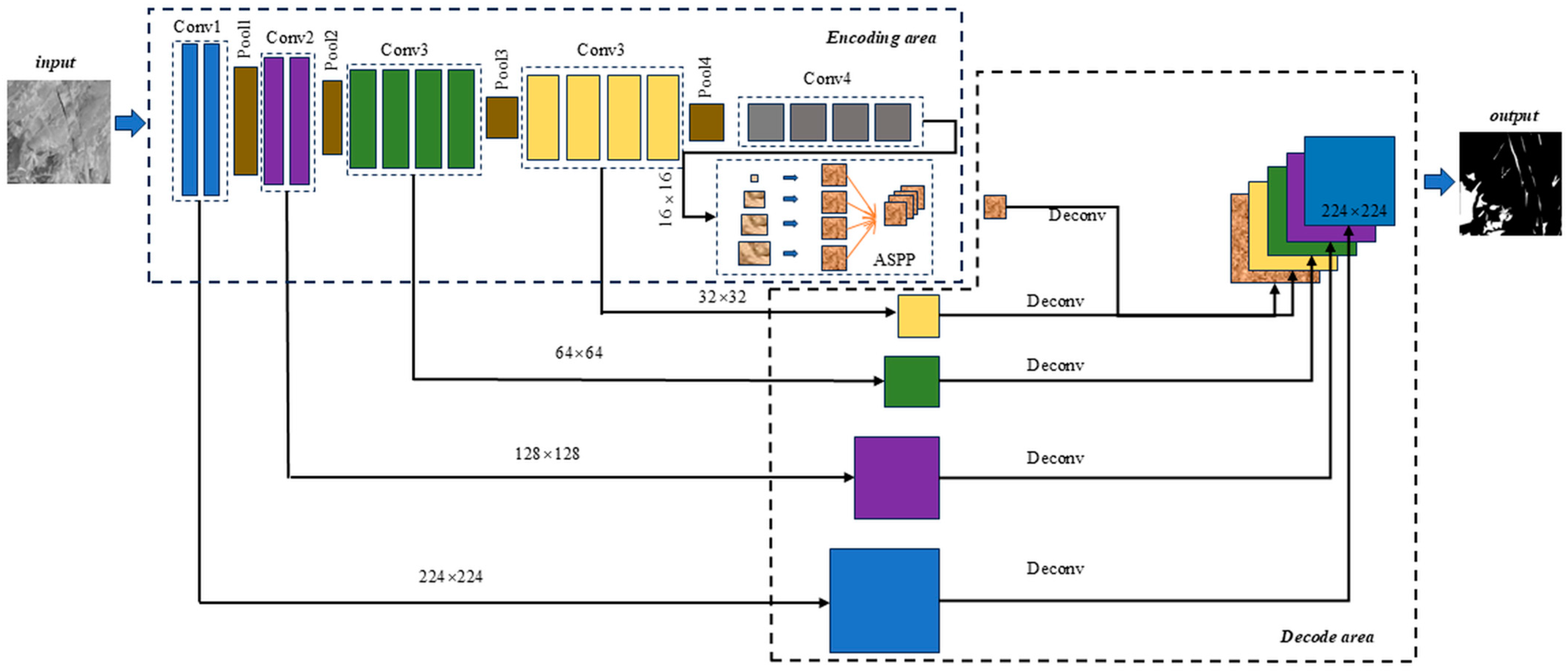
The input image is a 224 × 224 grayscale rock image with nodal fissure information. The image is preprocessed and normalized before being input into the model.
(2)
The encoder extracts multi-scale features from the image using several convolution and pooling layers. The process includes the following steps:
Conv1 and Pool1: After extracting the base texture features, the output size is reduced to 128 × 128 after the pooling operation.
Conv2 and Pool2: Deeper features are then extracted to capture the local properties of the nodes, giving an output size of 64 × 64.
Conv3 and Pool3: Higher-level features, like the overall shape and distribution of nodules, are then extracted, resulting in an output size of 32 × 32.
Conv4 and ASPP: At the final layer of the encoder, a 16 × 16 feature map is created by combining multi-scale context using a void space pyramid pooling module (ASPP).
The ASPP module expands the receptive field by using convolutions with different dilation rates. This helps the model capture nodal features at various scales, improving its ability to recognize both small and large nodules.
(3)
The decoder gradually upsamples the feature map and combines it with the encoder’s features using jump connections. This process helps restore the spatial resolution of the segmentation result. The decoder’s procedure is as follows:
Deconv1: The feature map is upsampled from 16 × 16 to 32 × 32 and combined with the matching 32 × 32 feature maps from the encoder layers.
Deconv2: The feature map is upsampled from 32 × 32 to 64 × 64 and combined with the matching 64 × 64 feature maps from the encoder.
Deconv3: The feature map is upsampled from 64 × 64 to 128 × 128 and combined with the matching 128 × 128 feature maps from the encoder.
Deconv4: The feature map is upsampled from 128 × 128 to 224 × 224, and the initial layer feature maps from the encoder are combined to preserve more edge details. Finally, the decoder creates a binary segmentation map, matching the size of the input image, using a 1 × 1 convolution. This map shows the locations of the nodules.
(4)
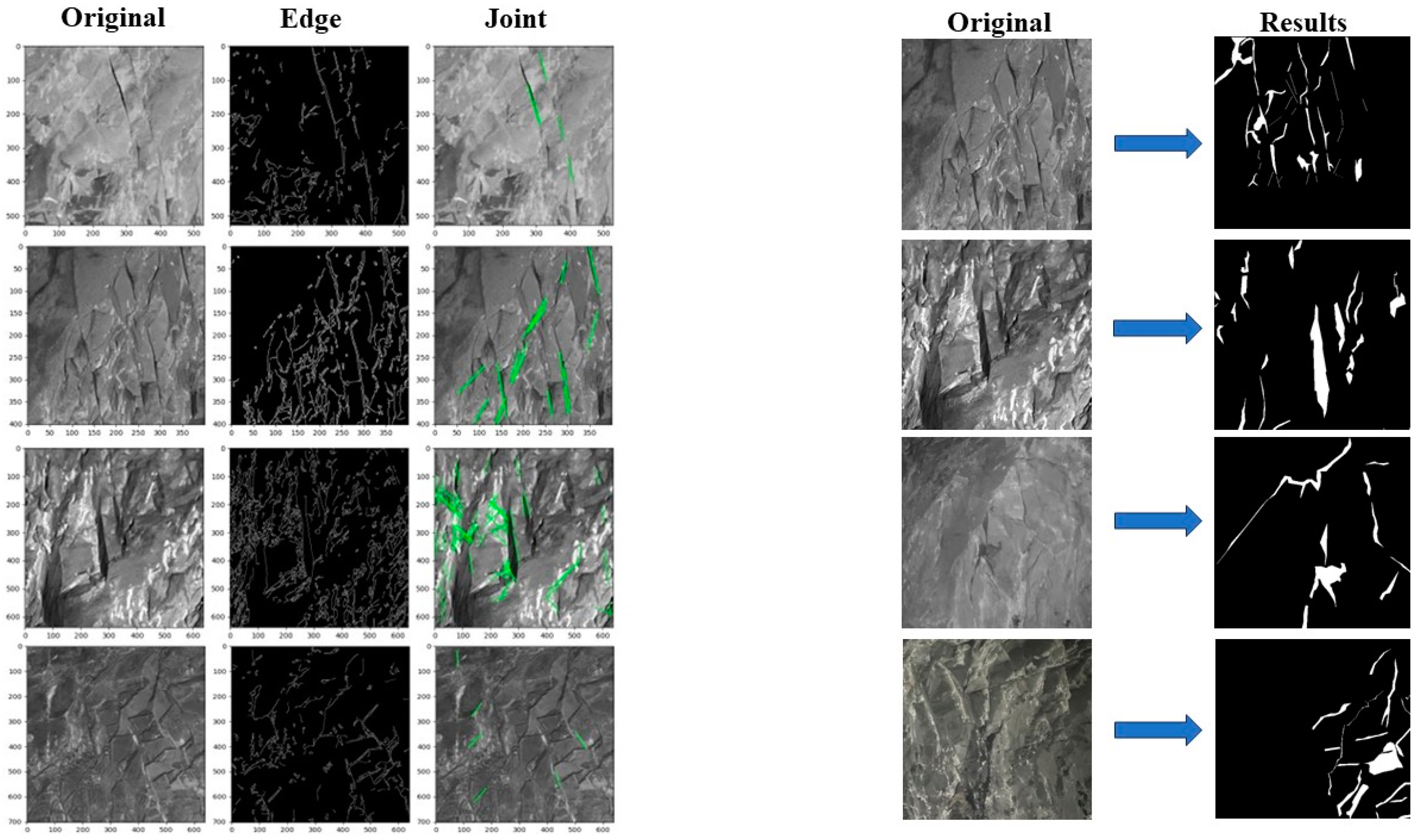
The segmentation results are output at the pixel level. Each pixel is classified as either a nodal region (target) in white or a non-nodal region (background) in black.

2.2. Model Optimization

Although FraSegNet improves nodal recognition [28], there are still areas for optimization, such as unstable training gradients, underused channel features, and incorrect learning rates. This study suggests three optimization strategies to improve training and accuracy: using ResNet101 as the backbone network, adding the SE attention mechanism, and applying a dynamic learning rate strategy.

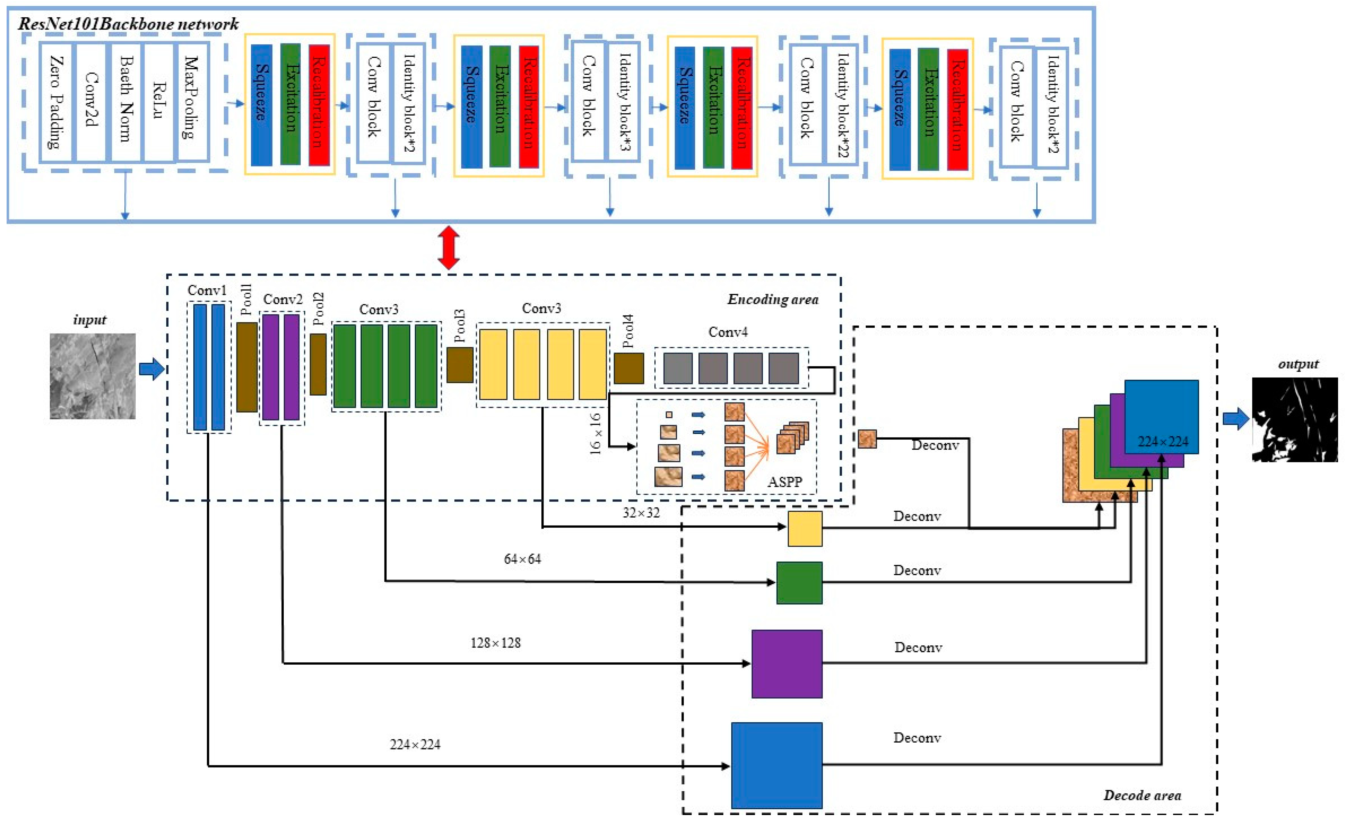
2.2.1. ResNet101 Backbone Network

In the original FraSegNet structure, the backbone network uses shallow convolutional modules for feature extraction. However, recognizing nodules requires a deep analysis of complex textures and multi-scale distributions, which shallow networks cannot capture well, especially deep semantic information. Shallow networks also have limited ability to express features, often missing detailed information, particularly in complex nodule shapes, which can result in key feature loss. ResNet101 is a 101-layer residual network that solves the gradient vanishing issue in deeper networks through residual connections. It also improves feature expression. The main backbone of ResNet101 is shown in Figure 2. The optimization method is as follows:
(1) The basic unit of ResNet101 is the residual block, which solves the gradient vanishing problem in deep networks using jump connections. These connections maintain continuity between shallow and deep features. ResNet101 has four stages, each with multiple residual modules. These modules gradually extract features, starting from low to high levels, reducing the feature map resolution while increasing feature dimensionality at each step. To speed up training and improve initial performance, ResNet101 uses ImageNet pre-trained weights as starting parameters, which are then fine-tuned on the rock body image dataset:
y = F ( x , W )
where x is the input feature.
F(x, W) is the feature mapping after convolution and nonlinear activation.
(2) In the nodule identification task, features at different scales are equally important for segmentation. So, the multi-layer feature outputs from ResNet101 are used for feature fusion: (1) Multi-scale feature extraction: Feature maps are extracted at different stages of ResNet101: Stage 1 (224 × 224 resolution): Extract low-level texture information. Stage 2 (112 × 112 resolution): Capture local structural features. Stage 3 (56 × 56 resolution): Extract mid-scale semantic information. Stage 4 (28 × 28 resolution): Aggregate global semantic features. (2) Jump connection: The multi-scale features from the encoder are passed to the decoder through jump connections. Combined with the upsampling in the decoder, this restores high-resolution segmentation results step by step.
(3) Since the feature dimensions and resolutions of ResNet101 are different from the original backbone network, the decoder of FraSegNet needs to be adjusted accordingly: (1) Increase the upsampling module in the decoder to gradually recover features from low to high resolution. (2) Merge the multi-scale features of the encoder using feature concatenation or attention mechanisms to ensure that the decoder fully uses the semantic information extracted by ResNet101.

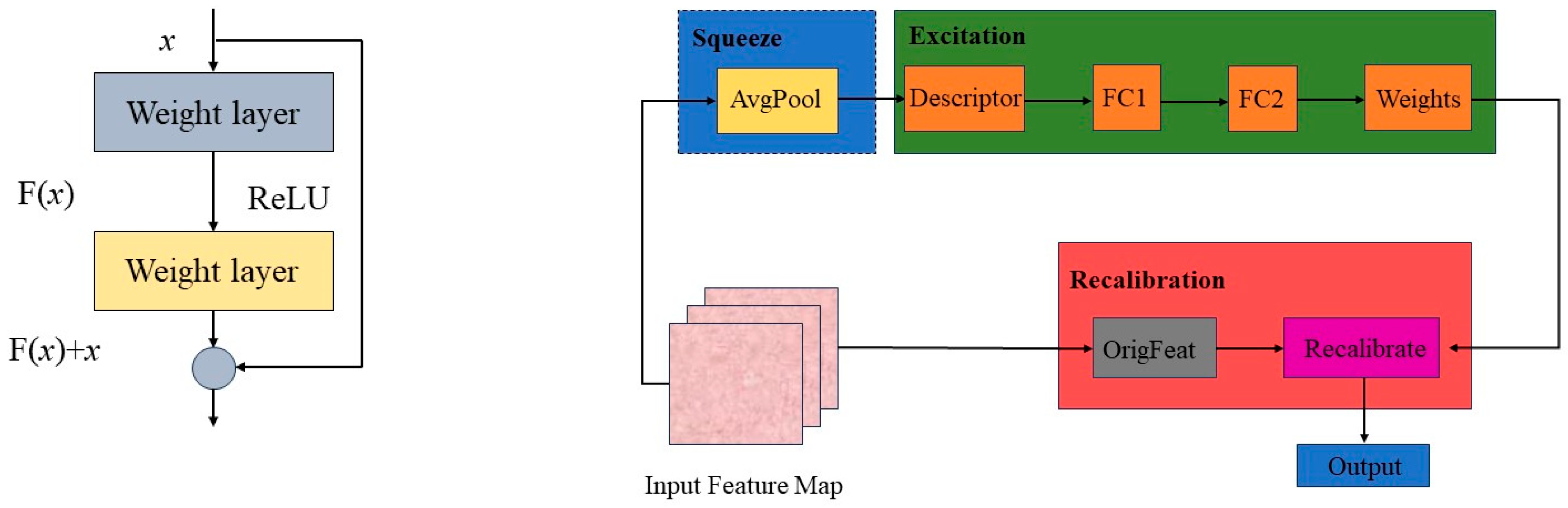
2.2.2. Introduction of the SE Attention Mechanism

In the nodule recognition task, rock body images often have rich background information (e.g., rock texture and noise) that can interfere with the model’s ability to accurately identify nodule regions. The original FraSegNet uses a uniform weighting approach for feature maps, which does not capture the importance of different channels dynamically, leading to poor differentiation between nodule and background features. The SE module improves the expression of key features and reduces redundant information by adjusting the weights of the feature channels.
The SE module has three main steps: (1) Squeeze: This operation pools the global average of each feature map, turning 2D feature maps into 1D channel descriptors to capture global spatial information. (2) Excitation: A fully connected layer learns the relationships between channels, followed by a sigmoid activation to create a channel-level attention map. (3) Recalibration: The generated channel weights are multiplied with the original feature map, adjusting the importance of each channel.
Incomplete connections in the fully connected layer during the Excitation of the SE module can lead to the following: 1. Failure of the attentional mechanism: The fully connected layer is used to learn the dependencies between channels, and if the connections are incomplete, the information of some channels may not be modeled correctly, leading to an imbalance in the allocation of attention. This may result in abnormal attention weights (too high or too low) for some channels, affecting the performance of the model. 2. Impaired gradient propagation: The fully connected layer of the SE module relies on parameter learning to adjust the channel weights, and if the connection is incomplete, the gradient may not be propagated correctly. This will affect the training of the whole model, making the SE module unable to effectively improve the feature expression ability. 3. Abnormal numerical computation: If the parameters of the fully connected layer are not initialized correctly or the connection is lost, this may lead to abnormal values such as NaN (Not a Number) or Inf (Infinity), which will affect the training and inference of the whole network. 4. Inability to correctly generate the channel attention maps: The output of the Excitation process is a channel-level attention vector that is used to weigh the input feature maps. If an error is made in the FC layer computation, it may result in the following: (i) The attention vector becomes all-zero (all channels are suppressed). (ii) The attention vector tends to be all-ones (no real adjustment effect). (iii) The attention values are not regularly distributed, resulting in the model not being able to focus on important features correctly. The structure of Squeeze-and-Excitation is shown in Figure 3.

2.2.3. Dynamic Learning Rate Strategy

A dynamic learning rate strategy addresses three main issues with FraSegNet—gradient oscillation with a high learning rate, slow training with a low learning rate, and lack of dynamic learning rate adjustment. This strategy adjusts the learning rate during training, leading to faster convergence and better final performance. The learning rate changes dynamically across training stages, speeding up convergence and improving the final results. The specific optimization method is as follows:
(1) Cosine annealing: During training, the learning rate is slowly reduced following a cosine function. At first, a higher learning rate helps with fast convergence, and later, the learning rate is gradually adjusted for better optimization.
η t = η m i n + 1 2 ( η m a x η m i n ) ( 1 + cos   ( t T π ) )
where
  • ηt is the current learning rate;
  • ηmax and ηmin are the maximum and minimum learning rates;
  • t is the current training iteration;
  • T is the total number of iterations.
(2) Warm-up strategy: The learning rate starts small and is gradually increased at the beginning of training. This helps prevent instability from sudden parameter updates.
The optimized FraSegNet network structure is shown in the Figure 4.

3. Evaluation Methods

3.1. Image Segmentation Evaluation Metrics

A combination of Intersection over Union (IoU) loss and Dice loss is used to improve segmentation accuracy and handle class imbalance:
L o s s = ν B C E   L o s s + μ I o U   L o s s + λ D i c e   L o s s
where BCE loss is used to compute the cross-entropy error between the predicted results and the ground truth labels.
Dice loss and IoU loss are employed to enhance sensitivity to small target regions.
The weight coefficients λ, μ, and ν are set to 0.5, 0.25, and 0.25, respectively.
The model performance is evaluated using these two metrics:
(1)
IoU (Intersection over Union): This metric measures the overlap between the predicted and ground truth regions. It is defined as follows:
I o U = T P T P + F P + F N
(2)
Dice Coefficient: This metric measures the similarity between the predicted segmentation and the ground truth, and is defined as follows:
D i c e = 2 × T P 2 × T P + F P + F N
The confusion matrix is also used to evaluate the performance of an image segmentation model. In segmentation, the classification result for each pixel fills the confusion matrix.
The basic form of the confusion matrix for image segmentation has four elements:
  • True Positive (TP): The number of pixels correctly predicted as the target class.
  • False Positive (FP): The number of pixels incorrectly predicted as the target class (background predicted as the target class).
  • False Negative (FN): The number of pixels incorrectly predicted as background (target class predicted as background).
  • True Negative (TN): The number of pixels correctly predicted as the background class.

3.2. Rock Mass Parameter Evaluation Metrics

The FraSegNet algorithm shows better nodal extraction accuracy and robustness after improving the backbone network, adding the attention mechanism, and using the dynamic learning rate strategy. However, to check if the improved algorithm extracts nodal features accurately, using only image segmentation metrics (e.g., IoU and F1-Score) is not enough. Verification should also be performed using actual mechanical criteria. The Barton–Bandis nodal parameter mapping and the Hoek–Brown strength criterion are proposed to validate FraSegNet’s accuracy in extracting nodal features, connecting the algorithm’s segmentation performance to the mechanical properties of the rock body.

Correlation Analysis of Nodal Cleavage Parameters Rock Mass Parameters

Enclosed rock characteristic parameters describe the distribution of structural and geometric features in the rock mass. These parameters are key indicators of the rock’s engineering properties. Common surrounding rock characterization parameters include the following: (1) Fracture Density: It is the total length of fractures per unit area, showing the level of fracture development. (2) Fracture Length: It is the linear length of a single fracture, which affects the continuity of the rock mass. (3) Fracture Width: It is the opening width of a fracture, which determines how much the rock mass’s stiffness and strength are weakened. (4) Fracture Dip Angle: It is the angle between the fracture and the horizontal plane, which affects the fracture’s sliding tendency. (5) Fracture Area: It is the total area of fractures in the two-dimensional projection, showing the distribution range of fractures.
Commonly used rock mechanics parameters include the following: (1) Density: It describes the mass distribution of the rock mass. (2) Bulk Modulus: It reflects the ability of the rock mass to deform under uniform pressure. (3) Shear Modulus: It describes the ability of the rock mass to resist shear deformation. (4) Elastic Modulus: It is the deformation capacity of the rock mass under axial stress. (5) Cohesion: It reflects the rock mass’s resistance to shear failure. (6) Friction Angle: It describes the sliding resistance of the rock mass. (7) Tensile Strength: It is the failure strength of the rock mass under tensile stress. (8) Poisson’s Ratio: It is the ratio of lateral deformation to axial deformation in the rock mass.
Higher fracture densities weaken the rock mass, reducing its cohesion, tensile strength, and elasticity. Fissures lower the strength and stiffness of the rock, increasing the risk of slippage and damage. As fissure width increases, the stiffness of the rock decreases, lowering the modulus of elasticity and shear modulus. Larger fissures allow more space for deformation, making it easier for the rock to deform and be damaged. The inclination angle of the fissures affects the rock’s tendency to slip. A larger inclination increases the risk of slippage and reduces the friction angle, affecting stability. Fissures also influence the rock’s deformation, especially under axial stress. The distribution, length, and width of the fissures affect the rock’s Poisson ratio, impacting its lateral deformation.

3.3. Barton–Bandis Parameter Mapping

In rock mechanics, the Barton–Bandis model is an empirical model used in geotechnical engineering to predict rock strength and deformation, especially for estimating rock body strength. Proposed by engineers Barton and Bandis in 1980, the model is mainly used to characterize rock strength under different environmental conditions and stress states [29,30].

3.3.1. Parameter Mapping Formula

To automate the conversion of fracture characteristics into rock mass mechanical parameters, a mapping relationship is created based on the Barton–Bandis theory and experimental analysis:
(1)
Density: Density decreases as fracture density increases, and this is shown by the following equation:
ρ = ρ 0 · exp   ( α · D )
where
  • ρ: The density of the fractured rock mass (kg/m3).
  • ρ0: The density of the intact rock (kg/m3), i.e., the original rock without fractures.
  • D: The fracture density, typically defined as the total length of fractures per unit area (m/m2).
  • α: The density decay coefficient quantifies the effect of fracture density on the overall rock mass density.
(2)
The formula for the cohesion (C) of a fractured rock mass, considering fracture density and area, is usually written as follows:
C = C 0 · exp   ( k · A J C S )
where
  • C: The cohesion of the fractured rock mass (in MPa).
  • C0: The cohesion of the intact rock (in MPa).
  • A: The fracture area (in m2), representing the total area of fractures in a given volume or unit area of rock.
  • D: The fracture density (in m/m2), defined as the total length of fractures per unit area.
  • k: The weakening coefficient quantifies the reduction in cohesion caused by the presence of fractures.
  • JCS: The peak normal stress on the fracture surface, related to the fracture’s resistance to shear along the fracture plane (in MPa).
(3)
The formula for the friction angle (φ) of a fractured rock mass, affected by the fracture dip angle (θ), is usually written as follows:
ϕ = ϕ 0 J R C · lg   ( σ n / J C S ) 1 + θ / k ϕ
where
  • Φ: The friction angle of the fractured rock mass.
  • Φ0: The initial friction angle of the intact rock.
  • JRC: The Joint Roughness Coefficient represents the roughness of the fracture surface.
  • σn: The normal stress on the fracture surface (in MPa).
  • θ: The dip angle of the fracture relative to the horizontal (in degrees).
  • kΦ: The influence coefficient accounts for the effect of fracture characteristics (such as roughness and orientation) on the friction angle.
Equations (7) and (8) describe in detail the effect of cohesion and friction angle on rock cohesion, and these parameters are the core part of the definition in the Coulomb–Mohr criterion.
(4)
The formula for the elastic modulus (E) of a fractured rock mass, considering fracture density (D) and fracture width (W), is usually written as follows:
E = E 0 · exp   ( 1 k E · D 1 + W / W C )
where
  • E: The elastic modulus of the fractured rock mass.
  • E0: The elastic modulus of the intact rock.
  • D: The fracture density, usually expressed as the total length of fractures per unit area (fracture length density).
  • W: The average fracture width.
  • Wc: The critical width of the fractures at which they close and the elastic modulus returns to that of the intact rock.
  • kE: The elastic modulus attenuation coefficient represents the rate at which the elastic modulus decreases as the fracture density increases.
The fracture closure critical width (Wc) is the threshold width at which fractures start to close, and the material behavior returns to that of the intact rock. The formula for calculating Wc usually takes into account the properties of the fractures and the rock material and is written as follows:
W c = 2 · σ n · ( 1 ν ) E
(5)
Shear modulus and bulk modulus are calculated using the elastic modulus and Poisson’s ratio of the rock mass:
G = E 2 ( 1 + ν ) ,   K = E 3 ( 1 2 ν )
(6)
Tensile Strength: The increase in fracture density and width reduces the tensile strength:
σ t = σ t 0 · exp   ( k t · D · W J C S )
where
  • σt: the tensile strength of the rock mass with fractures.
  • σt0: the tensile strength of the intact rock mass.
  • Kt: the attenuation coefficient.
Poisson’s ratio of a rock mass changes with the number of fractures. The link between Poisson’s ratio (ν) and fracture density (ρ) is shown in this equation:
ν = ν 0 · ( 1 β · D )
where
  • ν0: the Poisson’s ratio of the intact rock mass (without fractures).
  • β: the attenuation coefficient of Poisson’s ratio.
The equation includes the fracture roughness coefficient (JRC) and normal peak stress (JCS) based on the Barton–Bandis theory. It shows how fractures affect the rock’s mechanical properties by considering fracture density, width, and stress. The Table 1 and Table 2 gives the ranges for the JRC values.
Barton proposed an empirical formula to find the Joint Compressive Strength (JCS) of fractures. It is shown below:
J C S = U C S · R
where
  • UCS: Uniaxial compressive strength of the intact rock.
  • R: Fracture strength degradation factor influenced by weathering.

3.3.2. Obtaining the Attenuation Coefficients

Table 3 shows the mechanical properties of unfractured rock. Table 4 and Table 5 list the fracture and mechanical properties of eleven rock samples chosen using tunnel stratigraphic data. The attenuation coefficients come from Table 1, Table 2 and Table 3, using Equations (6)–(13), as shown in the Table 6.
The data in Table 1, Table 2, Table 3, Table 4, Table 5 and Table 6 are brought into Equations (6)–(14) to calculate the data in Table 7.

3.4. Hoek–Brown Criterion Parameter Transformation

The Hoek–Brown criterion, created by Evert Hoek and John W. Brown in 1980 [31], is a common strength model. It combines uniaxial compressive strength and geometric features to describe rock strength. This method helps in rock engineering design and is used to turn rock parameters into rock mass parameters. It gives a simple way to calculate rock mass properties based on geological conditions. Fracture data from the Barton–Bandis model can be used to find these properties. The results are then compared with those from the Hoek–Brown method to check if the model works well and ensures safety in engineering designs.

3.4.1. Hoek–Brown Model Parameter Calculation

RMR = 100 5 J d 10 log J s Adjustment   Factor
where
  • Jd: Joint density;
  • Js: Joint Spacing.
The adjustment factor in the Hoek–Brown model considers joint surface roughness, infill material properties, and hydrogeological conditions. These factors affect how the rock mass behaves, including its strength and stability. Adding the adjustment factor makes the model better at showing rock mass properties under different conditions.
The GSI value can be calculated using the formula below:
G S I = R M R 5
The Hoek–Brown model explains rock mass strength under different confining pressures. The main equation is shown below:
σ 1 = σ 3 + σ c ( m b σ 3 σ c + s ) a
where
  • σ1: Maximum principal stress;
  • σ3: Minimum principal stress (confining pressure);
  • σc: Uniaxial compressive strength of the intact rock;
  • mb: Rock mass strength parameter, representing the shear characteristics of the rock mass;
  • s: Rock mass integrity parameter;
  • a: Empirical parameter, describing the nonlinear behavior of the rock mass.
Calculation of Hoek–Brown Parameters:
The parameters mb,s, and a can be calculated using the following equations:
m b = m i · e x p   ( G S I 100 28 14 D )
s = e x p   ( G S I 100 9 3 D )
α = 0.5 + 1 6 ( exp   G S I 15 e x p   ( 20 ) )
where
  • mi: Rock material constant, determined experimentally;
  • D: Disturbance factor, reflecting the degree of engineering disturbance to the rock mass.
The Hoek–Brown model was adopted in this study because of its ability to describe nonlinear rock strength properties, especially for jointed rock bodies. Compared to the Mohr–Coulomb model, the Hoek–Brown model can better accommodate the mechanical properties of fractured rock bodies, especially the stress changes before and after rock rupture. In addition, combined with the joint parameters extracted from the Barton–Bandis model, the Hoek–Brown model is able to provide a more reasonable estimation of the mechanical parameters of the rock mass, which improves the accuracy of the stability analysis of the surrounding rock.

3.4.2. Conversion from Rock Parameters to Rock Mass Parameters

The link between rock density and rock mass density includes porosity:
ρ r o c k   m a s s = ρ r o c k ( 1 φ )
where
  • ρrock: Rock density;
  • φ: Porosity.
According to the Hoek–Brown model, the link between rock mass cohesion (crock mass) and intact rock cohesion (crock) can be found by transforming strength parameters:
c r o c k   m a s s = c r o c k · e x p   ( G S I 100 28 14 D )
where
  • D: Disturbance parameter, this article takes 0.9.
  • GSI: The Geological Strength Index is used to assess the quality of the rock mass.
In the Hoek–Brown model, the friction angle (θ) of the intact rock is connected to the strength parameter (mh) and the integrity parameter (S). The relationship is shown below:
tan θ r o c k   m a s s = tan θ r o c k · ( s · e x p   ( G S I 100 9 3 D ) )
The link between the rock’s elastic modulus (Erock) and the rock mass’s elastic modulus (Erock mass) in the Hoek–Brown model is shown below:
E r o c k   m a s s = E r o c k · ( 0.02 + 1 D 1 + exp   ( 60 + 15 D G S I 11 ) )
The link between the rock’s Poisson’s ratio (νrock) and the rock mass’s Poisson’s ratio (νrock mass) in the Hoek–Brown model is shown below:
ν r o c k   m a s s = ν r o c k + k
where
  • k: Empirical parameter is related to the rock type and joint characteristics.
The shear modulus (Grock) can be calculated using the elastic modulus (Erock) and Poisson’s ratio (νrock) with this formula:
G r o c k   m a s s = E r o c k   m a s s 2 ( 1 + ν r o c k   m a s s )
The bulk modulus (Krock) can be calculated from the elastic modulus (Erock) and Poisson’s ratio (νrock) using this formula:
K r o c k   m a s s = E r o c k   m a s s 3 ( 1 2 ν r o c k   m a s s )
The rock tensile strength (Trock) is linked to the Hoek–Brown parameters and can be shown as follows:
T r o c k = σ c i m b · ( G S I 100 ) a
where
  • σc: Compressive strength of the intact rock.
Using the nodal parameters from the optimized FraSegNet algorithm, rock mass parameters were found using the Barton–Bandis model. These were compared with the results from indoor tests using the Hoek–Brown model to check the accuracy of the extracted nodal features. This comparison helps confirm the FraSegNet algorithm’s ability to capture key geological parameters.

4. Reliability Analysis

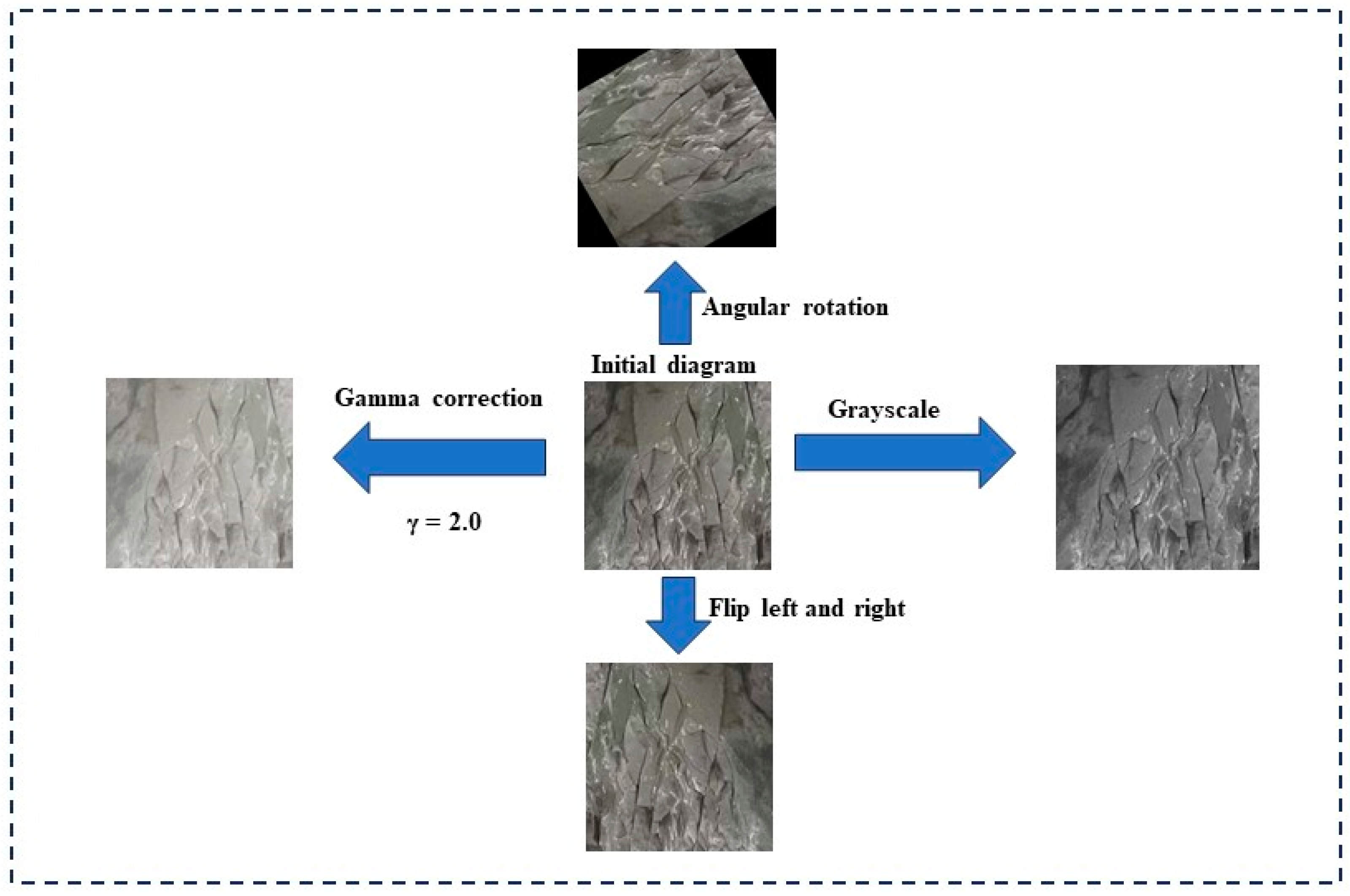
4.1. Dataset Creation

The palm face images were collected from the Huayingshan Tunnel Project in the Kangyu section of the Xiyu High-Speed Railway, captured using both smartphones and professional cameras before the first support phase. A total of 160 images were collected, representing a variety of perspectives and scales, which accurately depict the tunnel excavation scene. This diversity in image collection underscores the practicality of the nodal identification algorithm. Representative examples are illustrated in Figure 5.
The compressive strength of the rocks, as well as the values for RQD (Rock Quality Designation) and GSI (Geological Strength Index), are provided as follows: Compressive Strength: The compressive strength of the rock samples ranged from 160 MPa to 300 MPa, depending on the type of rock. This variation reflects differences in rock composition, fracture density, and other geological factors. RQD (Rock Quality Designation): The RQD values for the rock samples ranged from 52% to 73%, indicating the degree of fracturing in the rock mass. Higher RQD values suggest better-quality rock with fewer fractures. GSI (Geological Strength Index): The GSI values ranged from 42 to 35, providing a quantitative measure of the rock mass’s strength and quality, factoring in both the geological conditions and the characteristics of the rock fabric. These parameters are critical for understanding the mechanical properties of the rock mass and have been used to assess the tunnel’s excavation stability and the effectiveness of the nodal identification algorithm.
The Labelme software 4.5.7 was used to manually mark the joints in the tunnel palm face images. The labeled images were saved in two subfolders, matching the original image names, and stored in the same main directory. Since the original dataset was limited and varied, it was processed for consistency and accuracy. This included adjusting format and resolution, converting to grayscale, and augmenting the data. Common deep learning techniques like rotation, flipping (up, down, left, and right), and gamma correction were used to expand the dataset, as shown in Figure 6.
The augmented dataset includes 1000 images and 1000 labeled graphs (annotated with the Labelme software). It is split into three subsets: a training set, a testing set, and a validation set, following a 7:2:1 ratio. The training set, labeled “tra_”, has 700 images with labels; the testing set, labeled “tes_”, has 200 images with labels; and the validation set, labeled “val_”, contains 100 images with labels. Table 8 shows the number distribution of datasets.

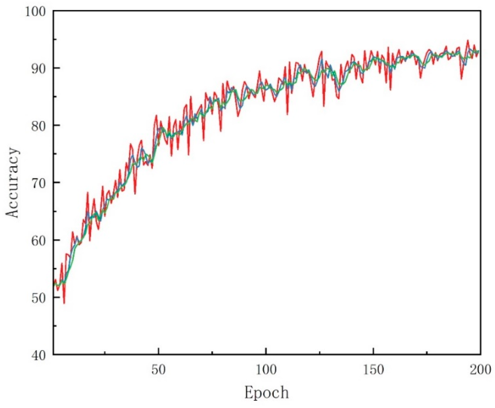
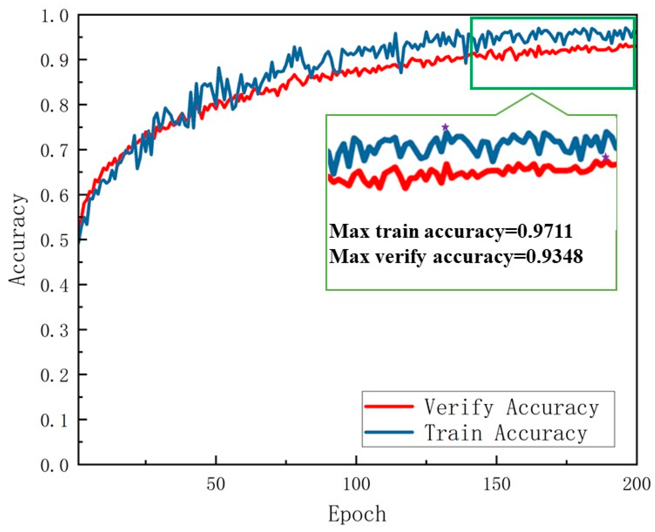
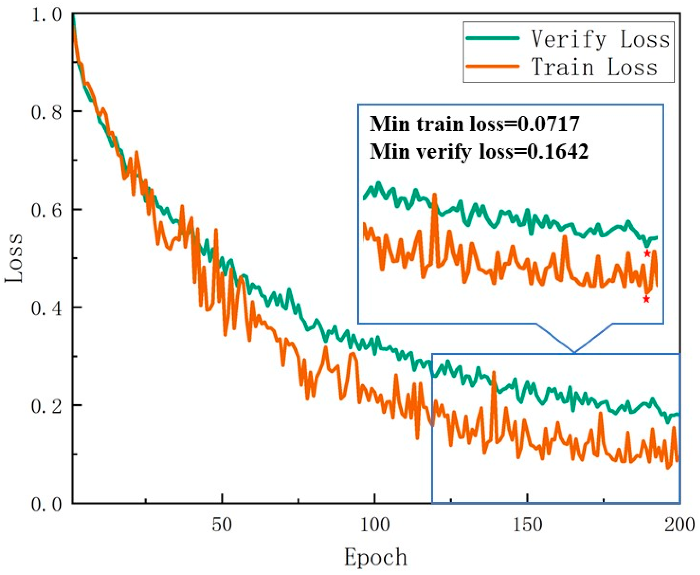
4.2. Performance Analysis Before and After Optimization

Using the same dataset for training, testing, and validation, we compared the performance of the FraSegNet model before and after optimization. Figure 7 and Table 9 illustrate significant enhancements in key performance metrics following optimization. Notably, the optimized FraSegNet model achieved improvements across multiple dimensions: increased accuracy, reduced training time, and faster testing time.
The optimized model demonstrated a marked increase in accuracy of 3.32%, resulting in more precise fracture extraction outcomes. Furthermore, the enhanced accuracy ensures that the model captures subtle fracture details with greater fidelity.
Efficiency gains were equally impressive: training time was reduced by approximately 42.3%, while testing time saw a reduction of 50%. These reductions underscore the dual benefits of the optimization process: enhanced model performance coupled with significantly improved computational efficiency.
In summary, the optimizations not only elevated the model’s accuracy but also substantially reduced the required computational resources, demonstrating a balanced enhancement in both performance and efficiency.
The optimized FraSegNet model is more robust against different levels of noise and lighting changes, as shown in Table 10. In the lighting test, the optimized model keeps higher accuracy and shows better detail and precision than the pre-optimized model. In the noise test, the optimized model handles Gaussian noise better, maintaining high accuracy in extracting nodal fissure edges even with high noise. In contrast, the pre-optimized model sees a large drop in accuracy, with blurred edges in high noise conditions. The generalization ability accuracy is shown in Figure 8.
To test the model’s ability to generalize, both the pre-optimized and optimized FraSegNet models were tested with K-fold cross-validation on three different datasets. The optimized model showed better stability across the datasets while maintaining high accuracy in nodal extraction.
Overall, the optimized FraSegNet model has clear improvements in accuracy, robustness, training efficiency, and generalization. It is better at extracting rock joints and fractures with more precision and reliability.

5. Experimental Results and Analysis

5.1. Data Analysis

The accuracy of the training and validation sets is shown using Python 3.10.12, and the accuracy curves for the nodal fissure features are shown in Figure 9. The loss rates of the training set and the validation set are shown in Figure 10.
The two charts illustrate the model’s accuracy and loss curves during both the training and validation phases. As the number of training epochs progressed, both metrics demonstrated consistent improvement, indicating effective learning and good generalization capability. Specifically, both training accuracy (reaching 0.9711 by the 150th epoch) and validation accuracy (reaching 0.9348 at the same point) exhibited steady upward trends, reflecting the model’s effective adaptation to the data. Although minor fluctuations were observed in validation accuracy, likely attributed to data complexity or overfitting concerns, the overall upward trajectory suggested robust generalization performance. The relatively small gap between the training and validation accuracies further indicated that significant overfitting was effectively mitigated.
For the loss rate, both the training and validation losses showed a consistent decline as training advanced, reflecting continuous improvement in the model’s predictive capabilities. By the final stages of training, the model achieved a training loss of 0.0717 and a validation loss of 0.1642, with these relatively low values suggesting a strong fit to the data. While minor fluctuations were present in the validation loss during intermediate and later training stages—typical behavior for deep learning models—the training loss curve maintained its smooth progression, indicating stable performance on the training set without significant oscillations.
Since feature extraction in deep learning models is often hard to interpret, this study employed the Grad-CAM algorithm [32] to generate activation heatmaps for the FraSegNet model. These visualizations provided insights into how different regions of the rock images influenced classification outcomes and verified whether the FraSegNet architecture successfully captured key features from the input data. The corresponding results are presented in Figure 11.
The first column shows the original image and the second column shows the heat map. The heat map highlights how different regions affect the predicted output, with darker areas indicating higher responses and greater contributions to the network. The results show that the optimized FraSegNet network accurately identifies the locations of dense nodal fissures.

5.2. Evaluation

This paper presents a validation method that integrates traditional metrics like IoU, the Dice coefficient, and the confusion matrix with a quantitative evaluation of rock parameters specifically tailored to address the practical demands of geoengineering applications. By incorporating the Barton–Bandis fracture parameter mapping with the Hoek–Brown strength model, the mechanical properties of the joint segmentation results can be evaluated. This combination of rock mass mechanical parameters and joint segmentation results provides a more holistic evaluation of the segmentation’s effectiveness, particularly in geoengineering, where the segmentation results are directly correlated with the rock mass’s mechanical properties. This integrated methodology significantly enhances the model’s practical applicability and relevance for real-world engineering scenarios.

5.2.1. Image Segmentation Evaluation

As shown in the figure, both the IoU and Dice coefficients steadily improve during training, showing the model’s increasing ability to optimize segmentation tasks. In the beginning, especially in the first 50 rounds, both IoU and Dice values improve quickly, indicating the model is learning basic features. This is typical for segmentation models, where early training focuses on learning basic contours and features. As training progresses (around 150 rounds), both metrics level off. Although the model is close to convergence, the rate of improvement slows, and segmentation performance stabilizes. The model achieves an IoU value of 0.9406, showing better coverage and more accurate boundary recognition of the target region. The highest Dice coefficient of 0.9877, close to the ideal 1.0, shows that the model fits the overlapping area well and handles overlaps and boundaries effectively. The loss rates of the training set and the validation set are shown in Figure 12.
To show the model’s segmentation performance, the confusion matrix is displayed in the figure, with darker colors showing higher values. This helps identify any classification bias and shows how the positive and negative classes are distributed. The confusion matrix is shown in Figure 13.
Accuracy is calculated as the ratio of correct predictions (true positives and true negatives) to the total number of samples. It is expressed as follows:
Accuracy = Predict   the   total   number   of   correct   samples Total   sample   size
The number of correctly predicted samples is the sum of the diagonal elements in the confusion matrix:
403 + 299 + 244 = 946 Accuracy = 946 1000 = 0.946 Precision P 1 = 403 403 + 8 + 1 = 0.978
The model performs well in overall classification with high accuracy, especially in recognizing joints accurately and consistently.

5.2.2. Rock Mass Parameter Characterization Evaluation

The study area was selected from the DK325+000 to DK327+100 section of the Huayingshan Tunnel. Three rock samples, labeled TS-1, TS-2, and TS-3, were collected at DK326+000. Data from the field, combined with deep learning and laboratory rock mechanics tests, helped systematically identify fissures, extract parameters, and estimate mechanical properties. This provided a scientific basis for the tunnel project’s design and construction. The detailed process of the study is outlined below. The sampling process and the location of sampling are shown in Figure 14 and Figure 15.
Fissure identification is performed using the FraSegNet deep learning model, which efficiently and accurately extracts fissure joints by training and validating collected rock body images. The model quickly identifies geometric features, such as spatial distribution, inclination, length, and width of nodules, greatly improving fissure identification efficiency and accuracy. The fracture extraction results for TS-1, TS-2, and TS-3 are shown in the figure.
Using the geometric features of the fissures extracted by FraSegNet, parameters such as length, width, dip, density, and area were calculated. The results, shown in the table, display the fracture characteristics of each rock sample in the study area. These results provide the needed inputs for estimating the mechanical parameters of the rock mass. Nodal extraction process and results by FraSegNet are shown in Figure 16. Table 11 shows the joint parameters.
By combining the extracted nodal parameters with the Barton–Bandis rock mechanics formulas, the mechanical properties of different rock samples—such as density, cohesion, friction angle, elastic modulus, shear modulus, bulk modulus, tensile strength, and Poisson’s ratio—were calculated. These results give detailed information on the rock mass properties, which are important for engineering design. They also serve as inputs for numerical simulations and stability analyses. Table 12 shows the rock mass mechanical parameters.
To study the differences in mechanical properties between rock and rock mass, the rock parameters were converted into rock mass parameters using a modified model based on joint density and area. This process used the Hoek–Brown criterion in the Rockdata software 2.2-1 [33]. The results show that fractures significantly weaken the rock mass properties, while the rock parameters more accurately reflect the material’s inherent characteristics. The revised data show that the cohesion, friction angle, and modulus of elasticity of the rock are much higher than those of the rock mass. At the same time, the shear modulus, bulk modulus, and tensile strength of the rock mass have improved. Table 13 and Table 14 show the Rock mechanical parameters and Rockmass mechanical parameters.
To assess the effectiveness of deep learning in engineering applications, the mechanical parameters of surrounding rock were analyzed and compared using the DK326+010 mileage section as a case study. The rock parameters extracted using deep learning and BartonBandis were compared with those obtained from indoor tests and converted using the Hoek–Brown criterion. The results showed minimal errors, indicating high consistency. Deviations in key parameters such as density, cohesion, friction angle, and modulus of elasticity were within the acceptable engineering range. This validation confirms that the deep learning-based method for extracting nodal parameters and estimating mechanical properties is highly accurate, reliable, and efficient, effectively replacing traditional manual methods.
The technical methods and data analysis in this study confirm that the optimized FraSegNet model identifies joints more accurately. This provides reliable technical support and serves as a valuable reference for future research on joint identification in complex engineering projects. Table 15 lists the data comparison.
In the comparison between the computer model predictions and the actual values, the following differences were observed for the various rock parameters:
Smallest Difference: The smallest difference observed across all parameters was in Poisson’s ratio, where the difference between the Barton–Bandis and Hoek–Brown models for each sample was consistently 0 (no difference), with values of 0.21 for TS-1 and 0.2 for TS-2 and TS-3. This indicates that both models gave identical results for this parameter.
Largest Difference: The largest difference observed was in elastic modulus for TS-2, with a difference of 0.04 GPa between the Barton–Bandis and Hoek–Brown models. This suggests that the models yielded slightly different results in terms of rock deformation capacity under axial stress, especially for sample TS-2. These differences illustrate the model’s performance across various mechanical properties, with certain parameters showing near-identical results, while others exhibit minor discrepancies, highlighting areas where further refinement of the models may be beneficial.
After data processing, the relative error, standard deviation, maximum error, and average error of the rock mass parameters obtained using the Barton–Bandis method and the Hoek–Brown criterion for the joints identified by FraSegNet were calculated. The average relative error between the two methods was 1.5%, well within the acceptable error range of 10%, ensuring the reliability and applicability of the results [34]. This shows that the joints identified by the FraSegNet model are highly accurate and suitable for engineering applications.

6. Conclusions

This paper presents an innovative nodal extraction method utilizing FraSegNet, integrated with the Hoek–Brown criterion, to effectively convert rock body parameters into rock mass parameters. The experimental results demonstrate that the method accurately extracts nodal information and efficiently transforms rock parameters, showcasing its substantial potential for broader applications. Future research could focus on improving the FraSegNet network’s performance in complex geological environments and refining the parameter transformation model to achieve more accurate mechanical analyses of rock bodies:
(1)
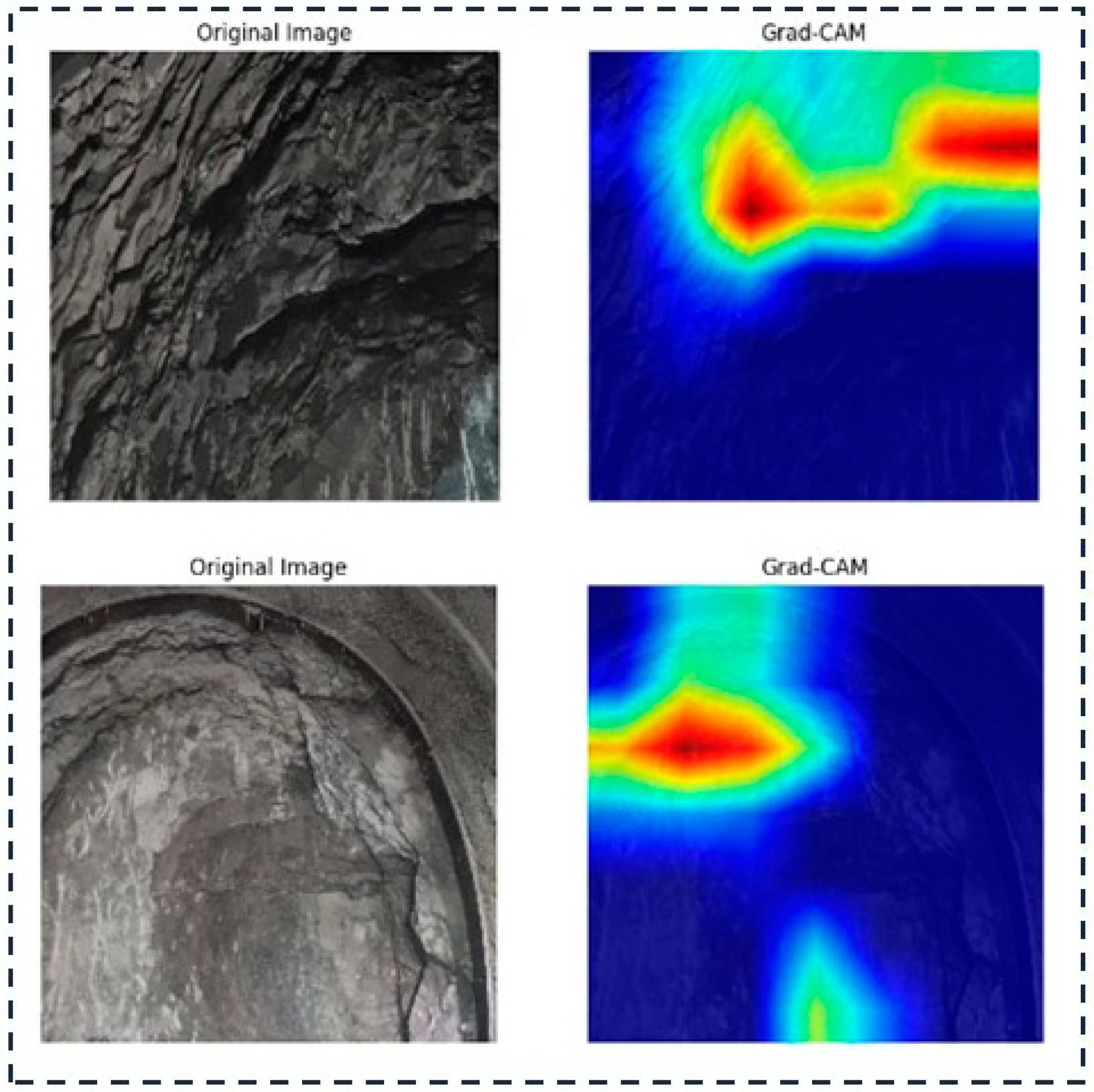
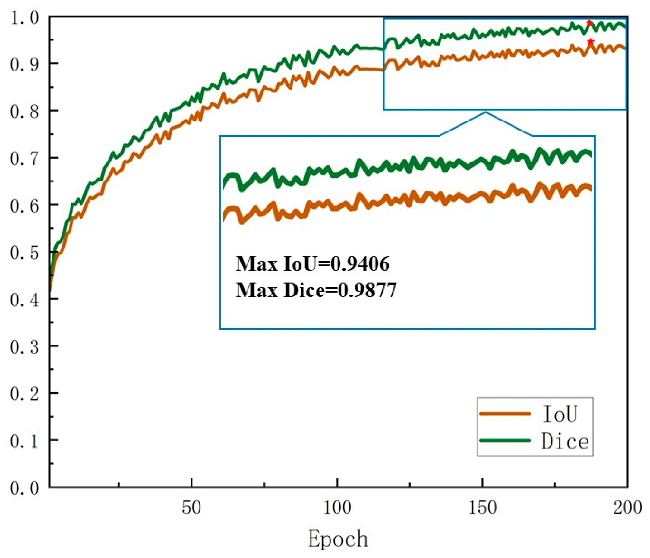
By incorporating the ResNet101 backbone, the SE attention mechanism, and a dynamic learning rate strategy, the optimized FraSegNet network enhances its feature extraction capabilities. This improvement is particularly beneficial for handling complex backgrounds and fine-grained targets. The experimental results show that the network achieves a training accuracy of 0.9711 and a minimum loss rate of 0.0717, with validation accuracy reaching 0.9348 and a minimum loss rate of 0.1642. The IoU and Dice coefficients for the automatic segmentation of nodal fissures stabilize at 0.94 and 0.98, respectively, demonstrating a notable enhancement in capturing fissure edge details compared to traditional segmentation methods. Additionally, the model excels in recognizing joints in tunnel surrounding rocks, with the confusion matrix and Grad-CAM visualization further validating its superior classification performance and ability to accurately assess dense joint areas.
(2)
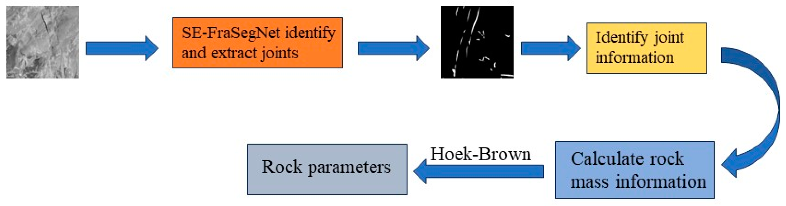
By combining the Barton–Bandis fracture parameter mapping with the Hoek–Brown strength criterion, this study establishes a clear relationship between the nodal features extracted by FraSegNet and the mechanical parameters of rock bodies. This integration provides reliable data support for future engineering applications, offering improvements in joint segmentation accuracy and a more precise reflection of rock body mechanical properties compared to traditional methods.
(3)
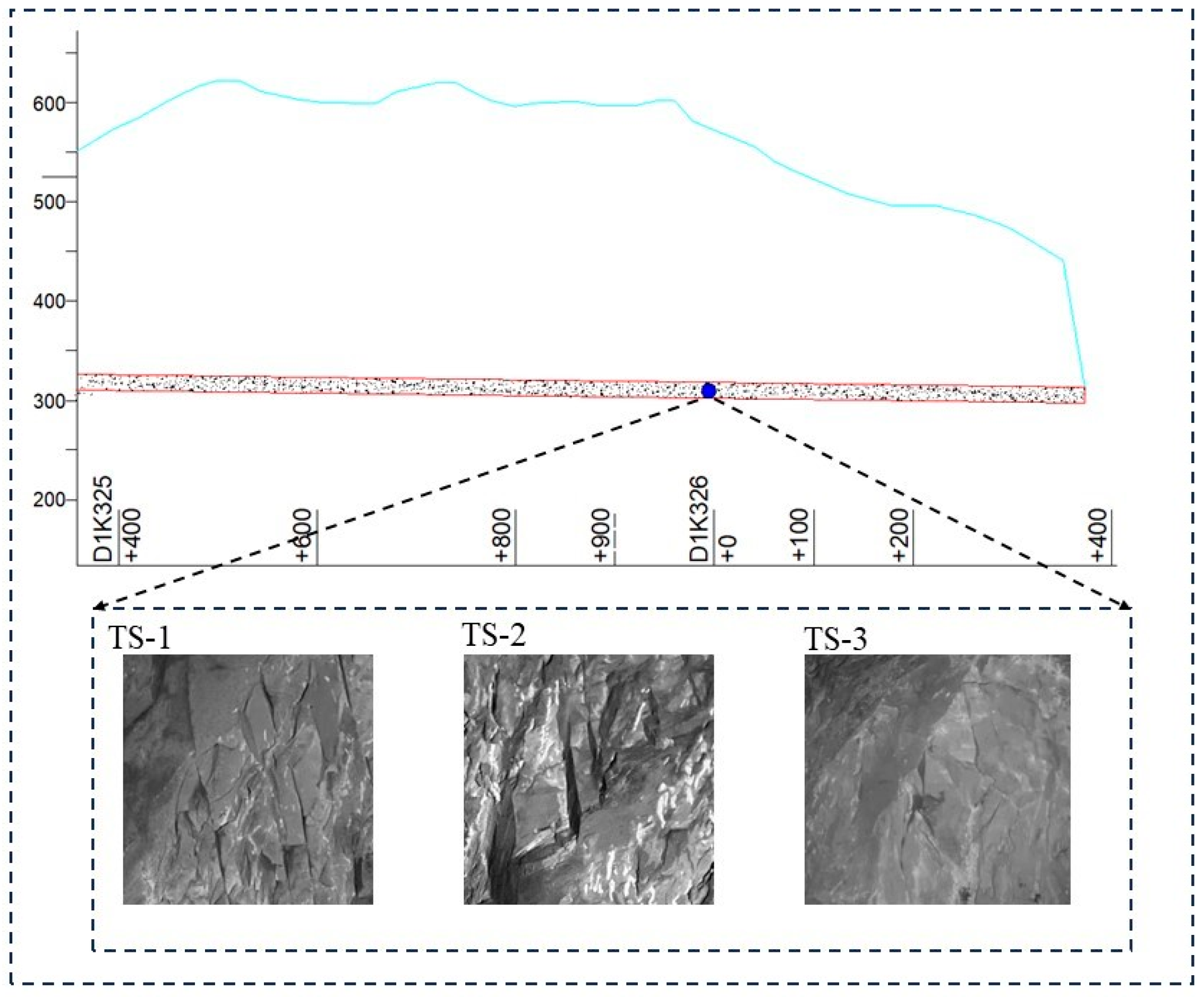
The proposed method was successfully tested in the Huayingshan Tunnel, validating its applicability and efficiency under complex geological conditions. It enhances the accuracy of rock joint and fissure identification, providing a reliable foundation for rock engineering design, stability analysis, and safety assessments. This approach holds significant value for both theoretical research and practical engineering applications.

Author Contributions

Data curation: Y.Z.; Formal analysis: Y.Z.; Funding acquisition: Y.Z.; Investigation: G.Z.; Project administration: G.Z.; Resources: G.Z.; Software: G.Z.; Supervision: G.Z.; Validation: Q.L.; Weiting-original draft: Q.L.; Visualization: X.Y.; Methodology: X.Y.; Writing-review&editing: H.Z. All authors have read and agreed to the published version of the manuscript.

Funding

1. National Natural Science Foundation of China, 52474098. 2. Natural Science Foundation of Hebei Province: Study on the dynamic disturbance effect and instability mechanism of rock failure with structural plane under true triaxial unloading. E2024209024.

Institutional Review Board Statement

Not applicable.

Informed Consent Statement

Not applicable.

Data Availability Statement

The original contributions presented in the study are included in the article. Further inquiries can be directed to the corresponding author.

Acknowledgments

We would like to thank Hebei Provincial Laboratory of Mining Industry Development with Safe Technology Priority for data support.

Conflicts of Interest

The authors declare no conflicts of interest.

References

  1. He, P.; An, J.; Shi, S.S.; Hu, J.; Wu, W.T.; Yan, Z.Q. Research on tunnel block collapse instability characteristics and support optimization design based on multi-scale modeling method of nodular rock body. J. Rock Mech. Eng. 2025, 1–15. [Google Scholar]
  2. Abbas, N.; Li, K.G.; Fissha, Y.; Khatti, J.; Geberegergis, M.B.; Cheepurupalli, N.R.; Taiwo, B.O.; Gebrehiwot, Z.; Kide, Y.; Chandrahas, N.S. Reliability analysis of support strategies in tunnel construction: Insights from geomechanical analysis of jointed rock masses. Results Earth Sci. 2024, 2, 100044. [Google Scholar] [CrossRef]
  3. Ge, C.H.; Li, P.F.; Zhang, M.J.; Li, Z. Eccentric load bearing performance of high bolt screw (HBS) active joints for prestressed internal supports in the subway excavation. Structures 2024, 70, 107876. [Google Scholar] [CrossRef]
  4. Yan, J.; Chen, J.; Zhang, Y.; Liu, Y.; Zhao, X.; Xue, J.; Zhu, C.; Mehmood, Q.; Wang, Q. Semi-automatic extraction of dangerous rock blocks from jointed rock exposures based on a discontinuity trace map. Comput. Geotech. 2023, 156, 105265. [Google Scholar] [CrossRef]
  5. Zhang, K.; Zhang, K.; Liu, W.; Xie, J. A novel DIC-based methodology for crack identification in a jointed rock mass. Mater. Des. 2023, 230, 111944. [Google Scholar] [CrossRef]
  6. Priest, S.D.; Hudson, J.A. Discontinuity spacing in rock. Int. J. Rock Mech. Min. Sci. Geomech. Abstr. 1976, 13, 135–148. [Google Scholar] [CrossRef]
  7. Zhang, L.; Einstein, H.H. Estimating the intensity of rock discontinuities. Int. J. Rock Mech. Min. Sci. 2000, 37, 819–837. [Google Scholar] [CrossRef]
  8. Wang, Y.; Zhou, J.; Chen, Q.; Chen, J.; Zhu, C.; Li, H. Automatic interpretation of geometric information of discontinuities and its influence on the stability of highly-jointed rock slopes. J. Rock Mech. Geotech. Eng. 2024. [Google Scholar] [CrossRef]
  9. He, P.; Yan, Z.; Wang, G.; Shi, S.; Zheng, C. Research on the multi-scale DFN-DEM equivalent modeling method for jointed rock masses and the collapse law of block structures. Tunn. Undergr. Space Technol. 2025, 157, 106316. [Google Scholar] [CrossRef]
  10. Ge, Y.; Yuan, S.; Chen, K.; Tang, H. Estimation of rock joint roughness using binocular stereo vision. Measurement 2024, 234, 114881. [Google Scholar] [CrossRef]
  11. Monteiro, B.A.A.; Canguçu, G.L.; Jorge, L.M.S.; Vareto, R.H.; Oliveira, B.S.; Silva, T.H.; Lima, L.A.; Machado, A.M.C.; Schwartz, W.R.; Vaz-de-Melo, P.O.S. Literature review on deep learning for the segmentation of seismic images. Earth-Sci. Rev. 2024, 258, 104955. [Google Scholar]
  12. Zhao, S.; Shadabfar, M.; Zhang, D.; Chen, J.; Huang, H. Deep learning-based classification and instance segmentation of leakage-area and scaling images of shield tunnel linings. Struct. Control. Health Monit. 2021, 1, e2732. [Google Scholar] [CrossRef]
  13. Cui, X.; Yan, E.C. A clustering algorithm based on differential evolution for the identification of rock discontinuity sets. Int. J. Rock Mech. Min. Sci. 2020, 126, 104181. [Google Scholar] [CrossRef]
  14. Lemy, F.; Hadjigeorgiou, J. Discontinuity trace map construction using photographs of rock exposures. Int. J. Rock Mech. Min. Sci. 2003, 40, 903–917. [Google Scholar] [CrossRef]
  15. Zou, Q.; Cao, Y.; Li, Q.; Mao, Q.; Wang, S. CrackTree: Automatic crack detection from pavement images. Pattern Recognit. Lett. 2012, 33, 227–238. [Google Scholar] [CrossRef]
  16. Ronneberger, O.; Fischer, P.; Brox, T. U-Net: Convolutional networks for biomedical image segmentation. In International Conference on Medical Image Computing and Computer-Assisted Intervention; Navab, N., Hornegger, J., Wells, W.M., Frangi, A., Eds.; Springer: Berlin/Heidelberg, Germany, 2015; pp. 234–241. [Google Scholar]
  17. He, K.; Zhang, X.; Ren, S.; Sun, J. Deep residual learning for image recognition. In Proceedings of the IEEE Conference on Computer Vision and Pattern Recognition, Las Vegas, NV, USA, 27–30 June 2016; pp. 770–778. [Google Scholar]
  18. Chen, L.C.; Papandreou, G.; Schroff, F.; Adam, H. Rethinking atrous convolution for semantic image segmentation. arXiv 2017, arXiv:1706.05587. [Google Scholar]
  19. Bordehore, J.L.; Riquelme, A.; Cano, M.; Tomás, R. Comparing manual and remote sensing field discontinuity collection used in kinematic stability assessment of failed rock slopes. Int. J. Rock Mech. Min. Sci. 2017, 97, 24–32. [Google Scholar] [CrossRef]
  20. Huang, H.; Zhao, S.; Zhang, D.; Chen, J. Deep learning-based instance segmentation of cracks from shield tunnel lining images. Struct. Infrastruct. Eng. 2020, 1, 1–14. [Google Scholar] [CrossRef]
  21. Xu, H.; Su, X.; Wang, Y.; Cai, H.; Cui, K.; Chen, X. Automatic bridge crack detection using a convolutional neural network. Appl. Sci. 2019, 9, 2867. [Google Scholar] [CrossRef]
  22. Dias, L.O.; Bom, C.R.; Faria, E.L.; Valentín, M.B.; Correia, M.D.; De Albuquerque, M.P.; De Albuquerque, M.P.; Coelho, J.M. Automatic detection of fractures and breakout patterns in acoustic borehole image logs using fast-region convolutional neural networks. J. Pet. Sci. Eng. 2020, 191, 107099. [Google Scholar] [CrossRef]
  23. Zhang, Y.; Chen, J.; Li, Y. Segmentation and quantitative analysis of geological fracture: A deep transfer learning approach based on borehole televiewer image. Arab. J. Geosci. 2022, 15, 300. [Google Scholar] [CrossRef]
  24. Liu, Y.; Liao, G.; Xiao, L.; Liang, Z.; Zhang, J.; Zhang, X.; Zhang, Z.; Zhou, J.; Li, G. Automatic fracture segmentation and detection from image logging using Mask R-CNN. In Proceedings of the SPWLA 63rd Annual Logging Symposium, Stavanger, Norway, 11–15 June 2022. [Google Scholar]
  25. Long, J.; Shelhamer, E.; Darrell, T. Fully convolutional networks for semantic segmentation. In Proceedings of the 28th IEEE Conference on Computer Vision and Pattern Recognition, Boston, MA, USA, 7–12 June 2015; pp. 3431–3440. [Google Scholar]
  26. Alghalandis, Y.F. ADFNE: Open source software for discrete fracture network engineering, two and three-dimensional applications. Comput. Geosci. 2017, 102, 1–11. [Google Scholar] [CrossRef]
  27. Chen, J.; Zhou, M.; Huang, H.; Zhang, D.; Peng, Z. Automated extraction and evaluation of fracture trace maps from rock tunnel face images via deep learning. Int. J. Rock Mech. Min. Sci. 2021, 142, 104745. [Google Scholar] [CrossRef]
  28. Bandis, S.; Lumsden, A.C.; Barton, N.R. Experimental studies of scale effects on the shear behavior of rock joints. Int. J. Rock Mech. Min. Sci. Geomech. Abstr. 1981, 18, 1–21. [Google Scholar] [CrossRef]
  29. Zhao, L.; Yu, C.; Cheng, X.; Zuo, S.; Jiao, K. A method for seismic stability analysis of jointed rock slopes using Barton-Bandis failure criterion. Int. J. Rock Mech. Min. Sci. 2020, 136, 104487. [Google Scholar] [CrossRef]
  30. Zhao, L.-H.; Zuo, S.; Li, L.; Lin, Y.-L.; Zhang, Y.-B. System reliability analysis of plane slide rock slope using Barton-Bandis failure criterion. Int. J. Rock Mech. Min. Sci. 2016, 88, 1–11. [Google Scholar] [CrossRef]
  31. Hoek, E.; Brown, E.T. Empirical strength criterion for rock masses. J. Geotech. Geoenviron. Eng. 1980, 106, 1013–1035. [Google Scholar] [CrossRef]
  32. Zhou, B.; Khosla, A.; Lapedriza, A.; Oliva, A.; Torralba, A. Learning deep features for discriminative localization. In Proceedings of the 2016 IEEE Conference on Computer Vision and Pattern Recognition (CVPR), Las Vegas, NV, USA, 27–30 June 2016. [Google Scholar]
  33. Hu, Y.; Sun, Z.; Ji, J. Pseudo-dynamic stability analysis of 3D rock slopes considering tensile strength-modified Hoek–Brown failure criterion: Seismic UBLA implementations. Eng. Geol. 2024, 343, 107786. [Google Scholar] [CrossRef]
  34. Taylor, J.R. An Introduction to Error Analysis: The Study of Uncertainties in Physical Measurements, 2nd ed.; University Science Books: Sausalito, CA, USA, 1997. [Google Scholar]
Figure 1. FraSegNet network structure.
Applsci 15 04314 g001
Figure 2. ResNet101 backbone network (* means multiplication in pixels).
Applsci 15 04314 g002
Figure 3. Squeeze-and-Excitation.
Applsci 15 04314 g003
Figure 4. Optimized FraSegNet network structure diagram.
Applsci 15 04314 g004
Figure 5. Typical palm face image.
Applsci 15 04314 g005
Figure 6. Schematic diagram of image data augmentation.
Applsci 15 04314 g006
Figure 7. Accuracy comparison before and after optimization (red line: optimize; blue line: initial; yellow line: the line shows the red and blue lines are at the same value).
Applsci 15 04314 g007
Figure 8. Generalization ability test.
Applsci 15 04314 g008
Figure 9. Training and validation set accuracy.
Applsci 15 04314 g009
Figure 10. Training set and validation set loss rate.
Applsci 15 04314 g010
Figure 11. Grid-CAM heatmap.
Applsci 15 04314 g011
Figure 12. IoU and Dice.
Applsci 15 04314 g012
Figure 13. Confusion matrix.
Applsci 15 04314 g013
Figure 14. Specific flow chart for extracting rock parameters.
Applsci 15 04314 g014
Figure 15. Schematic diagram of rock sample location.
Applsci 15 04314 g015
Figure 16. Nodal extraction process and results by FraSegNet.
Applsci 15 04314 g016
Table 1. Range of JRC values.
Fracture Surface RoughnessJRC Range
Very Smooth0–2
Slightly Rough4–8
Significantly Rough10–20
Extremely Rough>20
Table 2. Range of R values based on fracture surface condition.
Fracture Surface ConditionR-Value Range
No Weathering0.7–1.0
Slight Weathering0.4–0.6
Moderate Weathering0.2–0.4
Severe Weathering0.1–0.2
Table 3. Parameters of intact rock samples.
SampleDensity (g/cm3)Cohesion (MPa)Friction Angle (°)Elastic Modulus (GPa)Shear Modulus (GPa)Bulk Modulus (GPa)Tensile Strength (MPa)Poisson’s Ratio
Intact Rock Sample2.817.8442.3772.1533.2185.4312.330.27
Table 4. Parameters of rock joints and fissures.
Sample No.Fracture DensityFracture Length (m)Fracture Width (m)Fracture Dip Angle (°)Fracture Area (m2)
11.254.180.4827.425.51
22.41.140.88.791.93
31.960.990.2461.589.7
41.710.5439.617.77
50.811.590.6110.989.4
60.82.670.0944.578.96
70.622.220.633.096.02
82.231.530.2181.849.23
91.73.10.1123.290.98
101.920.780.9559.632.04
110.541.530.9728.050.55
Table 5. Parameters required for calculation.
Sample No.JCS/MPaJRCσn/MPaWc/cm
1651560.23
2671660.24
3621350.22
4741560.25
5681570.24
6691570.24
7741380.26
8651760.25
9671660.24
10631950.23
11661760.23
Table 6. Rock mass parameters.
Sample No.Density (g/cm3)Cohesion (MPa)Friction Angle (°)Elastic Modulus (GPa)Shear Modulus (GPa)Bulk Modulus (GPa)Tensile Strength (MPa)Poisson’s Ratio
12.391.0226.2238.9811.4782.672.10.26
22.274.2626.532.795.8582.2140.21
32.763.8334.596.6513.7238.629.50.25
42.363.9232.7512.018.9719.93.90.26
52.284.0937.747.0431.430.515.70.21
62.541.329.4446.3732.948.447.30.26
72.142.4322.3925.4326.4483.624.30.25
82.721.4634.2638.0632.2483.479.70.25
92.074.4535.2263.9932.7410.639.70.23
102.743.4931.2321.29.955.973.30.21
112.772.3235.4231.6729.0247.575.50.22
Table 7. Degradation coefficients of rock mass parameters.
Density0.125
Cohesion0.622
Friction Angle0.258
Elastic Modulus0.591
Tensile Strength0.521
Poisson’s Ratio0.121
Table 8. Distribution of the number of datasets.
Training SetTest SetValidation Set
Original Images700200100
Labels700200100
Table 9. Performance metrics before and after optimization.
Performance MetricPre-Optimization ModelPost-Optimization ModelImprovement
Accuracy90.21%93.25%+3.32%
Training Time37 h26 h−42.3%
Testing Speed2 images/s4 images/s−50%
RobustnessSlight DecreaseMore StableImprovement
StabilityHigh FluctuationsLow FluctuationsImprovement
Table 10. Robustness comparison.
Original ImagePre-Optimization ModelPost-Optimization Model
Increased BrightnessApplsci 15 04314 i001Applsci 15 04314 i002Applsci 15 04314 i003
Decreased BrightnessApplsci 15 04314 i004Applsci 15 04314 i005Applsci 15 04314 i006
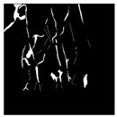
Strong Noise InterferenceApplsci 15 04314 i007Applsci 15 04314 i008Applsci 15 04314 i009
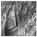
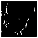
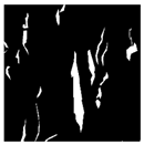
Weak Noise Interference
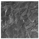
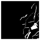
Applsci 15 04314 i010Applsci 15 04314 i011Applsci 15 04314 i012
Table 11. Joint parameters.
Rock SampleJoint Length (m)Joint Width (m)Joint Dip Angle (°)Joint DensityJoint Area (m2)
TS-114.171.544.320.0057.08
TS-26.220.6522.280.0023.11
TS-310.960.7532.110.0045.48
Table 12. Rock mass mechanical parameters.
Rock MassDensity (kg/m3)Cohesion (MPa)Friction Angle (°)Elastic Modulus (GPa)Shear Modulus (GPa)Bulk Modulus (GPa)Tensile Strength (MPa)Poisson’s Ratio
TS-124518.9639.6627.2910.4618.231.270.21
TS-224824.0532.4212.464.838.330.670.2
TS-324676.931.5621.378.2614.260.670.2
Table 13. Rock mechanical parameters.
Rock MassDensity (kg/m3)Cohesion (MPa)Friction Angle (°)Elastic Modulus (GPa)Shear Modulus (GPa)Bulk Modulus (GPa)Tensile Strength (MPa)Poisson’s Ratio
TS-1244517.639.4354.6321.0136.422.40.21
TS-224788.0637.2324.839.5516.551.120.2
TS-3246213.7531.7942.616.3828.41.270.2
Table 14. Rockmass mechanical parameters.
Rock MassDensity (kg/m3)Cohesion (MPa)Friction Angle (°)Elastic Modulus (GPa)Shear Modulus (GPa)Bulk Modulus (GPa)Tensile Strength (MPa)Poisson’s Ratio
TS-124458.839.6527.3210.51 18.211.20.21
TS-224784.0332.3512.424.788.280.660.2
TS-324626.8831.8221.38.1914.20.640.2
Table 15. Data comparison.
TS-1 Barton–BandisTS-1 Hoek–Brown TS-2 Barton–BandisTS-2 Hoek–BrownTS-3 Barton–BandisTS-3 Hoek–Brown
Density245124452482247824672462
Cohesion8.968.84.054.036.96.88
Friction Angle39.6639.4332.4232.3531.5631.79
Elastic Modulus27.2927.3212.4612.4221.3721.3
Shear Modulus10.4610.514.834.788.268.19
Bulk Modulus18.2318.218.338.2814.2614.2
Tensile Strength1.271.20.670.660.670.64
Poisson’s Ratio0.210.210.20.20.20.2
Disclaimer/Publisher’s Note: The statements, opinions and data contained in all publications are solely those of the individual author(s) and contributor(s) and not of MDPI and/or the editor(s). MDPI and/or the editor(s) disclaim responsibility for any injury to people or property resulting from any ideas, methods, instructions or products referred to in the content.

