Design of a Morphing Aircraft Based on Model Predictive Control

Abstract

Morphing aircraft can actively or passively change their shape in different flight environments and missions to ensure optimal flight performance at all flight stages, thereby enhancing environmental adaptability and meeting extensive multi-mission requirements. This paper proposes a stable flight control strategy for a variable-span aircraft based on Model Predictive Control (MPC). The Linear Parameter Varying (LPV) modeling approach is adopted to establish a longitudinal dynamic model that varies with the wingspan deformation rate. Without considering disturbances, a model predictive control strategy is designed to achieve dynamic stability control during flight. Considering the existence of composite disturbances during the morphing process, a robust model predictive control (RMPC) strategy is proposed, using set containment as the performance index. To verify the robustness of the control strategy, numerical tests are conducted under different wingspan deformation rates and disturbance intensities. The test results demonstrate that the RMPC strategy can effectively suppress external disturbances under various deformation rates, maintain stable flight speed and altitude, and ensure smooth transitions of critical flight state parameters such as angle of attack and pitch angle. These results validate the effectiveness of the proposed method.

1. Introduction

With the rapid advancement of aerospace technology, the performance requirements for aircraft have significantly increased. Traditional fixed-configuration aircraft are no longer capable of meeting the complex and diverse mission demands in both military and civilian applications [1]. In contrast, morphing aircraft, which enhance flight efficiency by dynamically adjusting their shape, have emerged as a promising solution. For instance, simulation experiments [2] have demonstrated that telescopic-wing aircraft can achieve greater roll angular velocity, maintain a larger control margin for control surfaces, and significantly improve maneuverability. This adaptability allows morphing aircraft to operate effectively across various environments and mission modes, such as cruise and maneuvering. However, the shape changes introduce significant nonlinear variations in the aircraft’s dynamic characteristics, transforming it into a nonlinear system dependent on geometric parameters. This property poses new challenges for flight control system design and has become a focal point of research [3,4,5,6,7].

To address the control challenges of morphing aircraft, various solutions have been proposed. Traditional approaches, such as gain scheduling or linear parameter-varying (LPV)-based robust control methods, combine multiple simple linear controllers to handle nonlinearity, thereby reducing system design complexity while meeting the requirements of large-envelope flight [8]. For example, the study in [9] analyzes the aerodynamic parameters and morphing relationships of variable-span aircraft, establishing a LPV model and designing a global controller using robust gain scheduling. Similarly, ref. [10] proposes a two-layer polyhedral LPV multi-objective control approach, where the first layer manages scheduling parameters and designs a gain-scheduled controller on vertex-uncertain systems, while the second layer ensures robustness in the closed-loop system. Additionally, ref. [11] introduces a class of finite-time convergent adaptive sliding mode controllers (ASMC) based on a linear time-varying parameter model to enhance system adaptability and control performance.

In the domain of nonlinear control, ref. [12] explores strategies for tailless aircraft in vertical flight, analyzing the following three controllers: an existing literature-based strategy, nonlinear dynamic inversion (NDI), and its incremental version (INDI). These controllers were implemented and tuned in simulations, validated through hardware-in-the-loop (HITL) tests, and applied in flight experiments. Furthermore, ref. [13] introduces a robust gain scheduling control strategy based on a sliding mode disturbance observer, improving closed-loop system robustness through disturbance compensation. Model predictive control (MPC) has also gained significant attention due to its excellent real-time optimization and constraint-handling capabilities, making it well-suited for controlling dynamically morphing aircraft [14,15]. For instance, ref. [16] designs a multi-model switching MPC controller for the longitudinal motion equilibrium transition of morphing aircraft, optimally coordinating morphing mechanisms, engine thrust, and elevator deflections to enhance flight performance, while ensuring state variables remain within predefined limits. Similarly, ref. [17] proposes a LPV-based MPC method for the transient deformation process of a bio-inspired folding-wing UAV, reformulating the online optimization problem into a quadratic programming (QP) problem for efficient real-time solutions. However, this study primarily focuses on pitch angle and airspeed tracking, without fully considering flight stability. To further enhance robustness, ref. [18] proposes an enhanced robust nonlinear MPC method that employs an incremental Lyapunov function to compensate for disturbance effects, and it efficiently handles constraints through online optimization. Although its computational cost is higher than that of nominal MPC, it ensures robustness and asymptotic stability in the presence of disturbances. Additionally, ref. [19] presents a novel robust MPC (RMPC) method for linear time-invariant systems with predictable disturbances and linear constraints on states and inputs, utilizing disturbance predictions in optimization to improve control performance. However, uncertainties such as sensor noise and environmental variations may limit its effectiveness.

Inspired by the aforementioned outstanding theories and discussions, this paper establishes a longitudinal nonlinear dynamic model for a variable-span aircraft based on multibody dynamics theory. The Jacobian linearization method is used, with wingspan variation selected as the scheduling parameter, to develop a LPV (Linear Parameter Varying) model for the longitudinal dynamics of the morphing aircraft. The LPV model is then discretized, and a Model Predictive Controller (MPC) is designed to ensure stable flight, assuming no system disturbances. Furthermore, considering the case where system disturbances do not decay to zero over time, this paper proposes a Robust Model Predictive Control (RMPC) strategy, using set containment as a performance metric. This approach enhances system stability and robustness against disturbances.

The remainder of this paper is organized as follows. Section 2 establishes the longitudinal nonlinear dynamic model and develops the LPV model. Section 3 designs both the MPC and RMPC controllers. Section 4 presents simulation results to validate the effectiveness of the controllers. Section 5 concludes the paper.

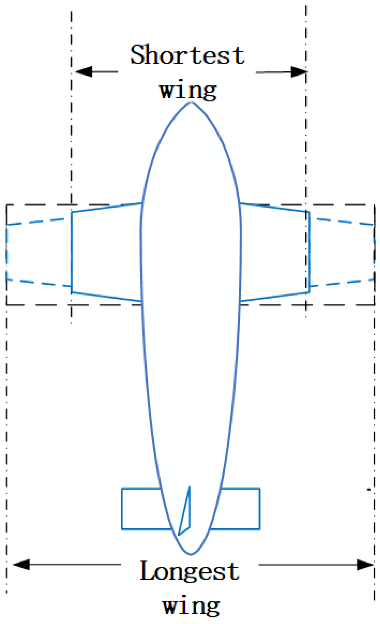
2. Mathematical Model of a Morphing Aircraft

2.1. Nonlinear Dynamic Model

The wingspan is directly related to the aspect ratio, significantly affecting the lift and drag characteristics of the aircraft. Based on the prototype aircraft, a variable-span aircraft is designed to be capable of symmetrically extending or retracting both wings during flight to adjust the wingspan. The maximum wingspan is twice the minimum wingspan, and the specific model parameters can be found in ref. [13]. Figure 1 presents a schematic diagram of the wingspan variation of a morphing aircraft.

Define the normalized description parameter of wingspan morphing for a variable-span aircraft as the wingspan morphing ratio ${\xi }_b$, expressed as follows:

$${\xi }_b={\displaystyle \frac{b-b_{min}}{b_{max}-b_{min}}}b$$

(1)

where b is the wingspan, and $b_{min}$ and $b_{max}$ are the minimum and maximum wingspans, respectively. Obviously, ${\xi }_b\in [0,1]$.

The wingspan morphing of the aircraft is a large-scale deformation with a relatively slow deformation rate. Since the sweep angle and dihedral angle of the morphing-wing aircraft are both approximately zero, the wingspan morphing does not affect the aircraft’s center of mass position, and its impact on the pitch moment of inertia is also negligible [20,21]. For aircraft with large-scale and slow morphing, the unsteady process of structural deformation has minimal deviation in the aerodynamic parameter simulation results. Therefore, the structural morphing process can be regarded as a series of continuous quasi-steady deformation states. The aerodynamic parameters under each static quasi-steady deformation state can be calculated through DATCOM simulations [9,22]. By selecting the altitude, Mach number, wingspan morphing rate, and pitch angle as operating points, the aerodynamic parameter data files obtained from DATCOM simulations for each operating point can be imported into the simulation software, allowing the visualization of phenomena through graphical representation.

As shown in Figure 2, at any operating point within the small angle-of-attack range $\alpha \in [-4^{\circ },{12}^{\circ }]$, a linear fit is applied to the lift coefficient $C_L$ and the pitching moment coefficient $C_m$, while a quadratic fit is applied to the drag coefficient $C_D$, yielding the following:

$$\left\{\begin{array}{c}{C}_L=C_{L_{\alpha =0}}+C_{L_{\alpha }}\alpha \hfill \\ C_D=C_{D_{\alpha =0}}+C_{D_{\alpha }}\alpha +C_{D_{{\alpha }^2}}{\alpha }^2\hfill \\ C_m=C_{m_{\alpha =0}}+C_{m_{\alpha }}\alpha \hfill \end{array}\right.$$

(2)

where $C_{L_{\alpha }=0}$, $C_{D_{\alpha }=0}$, and $C_{m_{\alpha }=0}$ represent the lift coefficient, drag coefficient, and pitching moment coefficient at zero angle of attack, respectively. $C_{L_{\alpha }}$, $C_{D_{\alpha }}$, and $C_{m_{\alpha }}$ denote the aerodynamic derivatives of lift, drag, and pitching moment with respect to the angle of attack, while $C_{{D_{\alpha }}^2}$ is the second-order aerodynamic derivative of drag with respect to the angle of attack.

By performing a least-squares fit of the longitudinal aerodynamic coefficients $C_L$, $C_D$, and $C_m$ at various operating points in the form of Equation (2) with respect to $\alpha$, and incorporating the longitudinal control derivatives and dynamic derivatives obtained from DATCOM simulation calculations, the overall longitudinal aerodynamic coefficient relationships can be established as follows:

$$\left\{\begin{array}{c}{C}_L=C_{L_{\alpha =0}}+C_{L_{\alpha }}\alpha +C_{L_{{\delta }_e}}{\delta }_e+C_{L_q}{\displaystyle \frac{c_{\mathrm{A}}}{2V}}q\hfill \\ C_D=C_{D_{\alpha =0}}+C_{D_{\alpha }}\alpha +C_{D_{{\alpha }^2}}{\alpha }^2\hfill \\ C_m=C_{m_{\alpha =0}}+C_{m_{\alpha }}\alpha +C_{m_{{\delta }_e}}{\delta }_e+C_{m_q}{\displaystyle \frac{c_{\mathrm{A}}}{2V}}q\hfill \end{array}\right.$$

(3)

where ${\delta }_e$ is the elevator deflection angle, q is the pitch rate, and $c_A$ is the mean aerodynamic chord of the wing. $C_{L_{{\delta }_e}}$ and $C_{m_{{\delta }_e}}$ are the aerodynamic derivatives of the lift and pitching moment with respect to elevator deflection, while $C_{L_q}$ and $C_{m_q}$ are the aerodynamic derivatives of the lift and pitching moment with respect to the pitch rate.

A variable-span aircraft follows a general morphing pattern, allowing the establishment of a conventional six-degree-of-freedom dynamic model. Therefore, the longitudinal nonlinear dynamic model of the variable-span aircraft is given as follows:

Some large-deformation aircraft, such as folding-wing and variable-sweep aircraft, require a multibody dynamics model to reasonably describe the effects of structural changes. However, conventional six-degree-of-freedom (6-DOF) dynamic models can still be used for general morphing configurations [9,23]. Based on the research objectives of this study, the following assumptions are made:

• The curvature of the Earth’s surface is neglected, adopting the so-called “flat Earth assumption”.
• The ground coordinate system is considered an inertial reference frame.
• The gravitational acceleration g is treated as a constant, ignoring variations with altitude.
• The morphing aircraft is assumed to be a rigid body, and its mass m remains constant throughout the entire flight process, including the structural morphing phase.
• The engine of the morphing aircraft is installed along the body’s longitudinal axis, and the thrust T passes through the aircraft’s center of mass with zero offset angle. This means the thrust acts only along the longitudinal axis and does not generate thrust-induced moments.
• The morphing aircraft performs level, sideslip-free flight, satisfying $\varphi =0$ and $\beta =0$, where $\varphi$ is the roll angle, $\beta$ is the sideslip angle, and p and r are the roll rate and yaw rate, respectively.

Therefore, the longitudinal nonlinear dynamic model of the morphing aircraft is formulated as follows:

$$\left\{\begin{array}{c}\dot{V}={\displaystyle \frac{1}{m}}Tcos\alpha -{\displaystyle \frac{1}{m}}D\left({\xi }_b\right)-gsin(\theta -\alpha )\hfill \\ \dot{\alpha }=-{\displaystyle \frac{1}{mV}}Tsin\alpha -{\displaystyle \frac{1}{mV}}L\left({\xi }_b\right)+q+{\displaystyle \frac{1}{V}}gcos(\theta -\alpha )\hfill \\ \dot{\theta }=q\hfill \\ \dot{q}={\displaystyle \frac{1}{I_y}}M\left({\xi }_b\right)\hfill \\ \dot{h}=Vsin(\theta -\alpha )\hfill \end{array}\right.$$

(4)

where L, D, and M represent the aerodynamic lift, drag, and pitching moment, respectively. m is the aircraft mass, g is the gravitational acceleration, and $I_y$ is the pitch moment of inertia. The thrust T is described by a simple linear relationship $T=T_{{\delta }_t}{\delta }_t$, where $T_{{\delta }_t}$ is the thrust coefficient, and ${\delta }_t$ is the throttle setting.The expressions for aerodynamic forces and moments are given as follows:

$$\left\{\begin{array}{cc}& L\left({\xi }_b\right)=Q{S}_w{C}_L({\xi }_b,h,M_a,\alpha ,{\delta }_e,q)\hfill \\ & D\left({\xi }_b\right)=Q{S}_w{C}_D({\xi }_b,h,M_a,\alpha )\hfill \\ & M\left({\xi }_b\right)=Q{S}_w{C}_m({\xi }_b,h,M_a,\alpha ,{\delta }_e,q)\hfill \end{array}\right.$$

(5)

where ${\delta }_e$ represents the elevator deflection angle. $Q=0.5\rho V^2$ is the dynamic pressure, $\rho$ is the air density, and $S_w$ is the reference wing area.

2.2. LPV Description of Nonlinear Systems

LPV systems are a class of linear systems whose models depend on measurable varying parameters and can describe the global behavior of the system along the varying parameter trajectory [24]. From Equation (5), it can be seen that, compared to conventional aircraft, the nonlinear dynamic model of the variable-span aircraft introduces the wingspan morphing ratio as an additional factor. To facilitate understanding and subsequent analysis, this nonlinear dynamic model is reformulated into the following affine nonlinear system form:

$$\left\{\begin{array}{c}\dot{\mathit{x}}\left(t\right)=f(\mathit{x}\left(t\right),{\xi }_b)+g(\mathit{x}\left(t\right),{\mathit{\xi }}_b)\mathit{u}\left(t\right)\hfill \\ \mathit{y}\left(t\right)=\mathit{x}\left(t\right)\hfill \end{array}\right.$$

(6)

where $\mathit{x}\left(t\right)={\left[\begin{array}{ccccc}V& \alpha & \theta & q& h\end{array}\right]}^{\mathrm{T}}$, which is the state vector; and $\mathit{u}\left(t\right)={\left[\begin{array}{cc}{\delta }_e& {\delta }_t\end{array}\right]}^{\mathrm{T}}$, which is the input vector.

The Jacobian linearization method is employed to construct the LPV model of the longitudinal nonlinear dynamics of the variable-span aircraft, with the wingspan morphing ratio selected as the scheduling parameter.

Neglecting compound disturbances, the modeling process proceeds as follows. First, a steady-level flight condition at an altitude of 5000 m and a velocity of 40 m/s is selected. Eleven reference equilibrium points are determined, corresponding to wingspan morphing ratios varying from 0 to 1 in increments of 0.1, and the trim states are computed. Next, the relationships between the angle of attack, elevator deflection, and thrust with respect to the wingspan morphing ratio are fitted using the least squares method to obtain analytical expressions. Finally, at each reference equilibrium point, the small-perturbation linearization matrices are computed using MATLAB R2023a and fitted as functions of the wingspan morphing ratio, establishing the nominal LPV model for the longitudinal dynamics of the aircraft.

$$\left\{\begin{array}{c}\Delta \dot{\mathit{x}}\left(t\right)=({\mathit{A}}_0+{\mathit{A}}_1{\tilde{\xi }}_b)\Delta \mathit{x}\left(t\right)+\mathit{B}\Delta \mathit{u}\left(t\right)\hfill \\ \Delta \mathit{y}\left(t\right)=\Delta \mathit{x}\left(t\right)\hfill \end{array}\right.$$

(7)

where $\Delta \mathit{x}\left(t\right)={\left[\begin{array}{ccccc}\Delta V& \Delta \alpha & \Delta \theta & \Delta q& \Delta h\end{array}\right]}^{\mathrm{T}}$, which is the state vector; and $\Delta \mathit{u}\left(t\right)={\left[\begin{array}{cc}\Delta {\delta }_e& \Delta {\delta }_t\end{array}\right]}^{\mathrm{T}}$, which is the input vector. Let ${\mathit{A}}_0$ be the nominal system matrix, ${\mathit{A}}_1$ the parameter - dependent term, and $\mathit{B}$ the control input matrix. $\Delta \mathit{x}\left(t\right),\Delta \mathit{u}\left(t\right),$ and $\Delta \mathit{y}\left(t\right)$ are expressed in incremental form, as follows:

$$\left\{\begin{array}{c}\Delta \mathit{x}\left(t\right)=\mathit{x}\left(t\right)-{\mathit{x}}_{\mathrm{e}}\left(t\right)\hfill \\ \Delta \mathit{u}\left(t\right)=\mathit{u}\left(t\right)-{\mathit{u}}_{\mathrm{e}}\left(t\right)\hfill \\ \Delta \mathit{y}\left(t\right)=\mathit{y}\left(t\right)-{\mathit{y}}_{\mathrm{e}}\left(t\right)\hfill \end{array}\right.$$

(8)

where $\mathit{x}\left(t\right),\mathit{u}\left(t\right),$ and $\mathit{y}\left(t\right)$ represent the actual values, and ${\mathit{x}}_{\mathrm{e}}\left(t\right),{\mathit{u}}_{\mathrm{e}}\left(t\right),$ and ${\mathit{y}}_{\mathrm{e}}\left(t\right)$ represent the trimmed values.

$${\mathit{x}}_{\mathrm{e}}\left(t\right)=\left[\begin{array}{c}{V}_e\hfill \\ {\alpha }_e\left({\xi }_b\right)\hfill \\ {\theta }_e\left({\xi }_b\right)\hfill \\ q_e\hfill \\ h_e\hfill \end{array}\right]=\begin{array}{c}\left[\begin{array}{c}40\\ -0.0546{\xi }_b^3+0.1626{\xi }_b^2-0.2282{\xi }_b+0.1655\\ -0.0546{\xi }_b^3+0.1626{\xi }_b^2-0.2282{\xi }_b+0.1655\\ 0\\ 5000\end{array}\right]\end{array}$$

(9)

$${\mathit{u}}_{\mathrm{e}}\left(t\right)=\left[\begin{array}{c}{\delta }_{e_e}\left({\xi }_b\right)\hfill \\ {\delta }_{t_e}\left({\xi }_b\right)\hfill \end{array}\right]=\left[\begin{array}{c}0.0071{\xi }_b^3-0.0254{\xi }_b^2-0.0969{\xi }_b-0.2687\\ -31.4718{\xi }_b^3+79.9797{\xi }_b^2-75.5495{\xi }_b+54.9813\end{array}\right]$$

(10)

Neglecting composite disturbances, the longitudinal LPV model for the stable flight of the morphing - wing aircraft is formulated as follows:

$$\left\{\begin{array}{c}\Delta \dot{\mathit{x}}\left(t\right)=\mathit{A}\left({\xi }_b\right)\Delta \mathit{x}\left(t\right)+\mathit{B}\Delta \mathit{u}\left(t\right)\hfill \\ \Delta \mathit{y}\left(t\right)=\Delta \mathit{x}\left(t\right)\hfill \end{array}\right.$$

(11)

where $\mathit{A}\left({\xi }_b\right)={\mathit{A}}_0+{\mathit{A}}_1\left({\xi }_b\right)$ represents the state matrix of this linear parameter - varying (LPV) system, which varies with the scheduling parameter ${\xi }_b$.

3. Controller Design

3.1. Model Predictive Controller Design

Model predictive control (MPC) predicts the system state and computes control commands in a receding horizon optimization manner while satisfying state constraints [25,26,27]. At each sampling instant, MPC solves a finite-horizon optimization problem to compute the optimal control sequence. For discrete-time systems, MPC reformulates Equation (3) into its discrete form, resulting in the following state-space equations: For discrete-time systems, Equation (11) is rewritten in discrete form, yielding the following state-space equation:

$$\Delta \mathit{x}(k+1)=\mathit{A}\left({\xi }_b\right)\Delta \mathit{x}\left(k\right)+\mathit{B}\Delta \mathit{u}\left(k\right)$$

(12)

The values of ${\xi }_b$ in the discrete system come from $[0,0.1,0.2,0.3,0.4,0.5,0.6,0.7,0.8,0.9,1]$. Consequently, in the discrete system, the state matrix $\mathit{A}\left({\xi }_b\right)$ can be regarded as a constant matrix. The control vector $\Delta \mathit{u}\left(k\right)$ is represented as $\mathit{u}\left(k\right)$, while the state vector $\Delta \mathit{x}\left(k\right)$ is represented as $\mathit{x}\left(k\right)$, for simplicity’s sake. The equation above can also be expressed as follows:

$$\mathit{x}(k+1)=\mathit{A}\mathit{x}\left(k\right)+\mathit{B}\mathit{u}\left(k\right)$$

(13)

Transforming the tracking problem into a stable control problem based on the error signal, we consider the initial time step as k and the prediction horizon as $N_p$. The quadratic performance index is defined as follows:

$$J={\displaystyle \frac{1}{2}}{\mathit{x}}_{\left[N_p\right]}^{\mathrm{T}}\mathit{S}{\mathit{x}}_{\left[N_p\right]}+{\displaystyle \frac{1}{2}}\sum _{k=0}^{N_p-1}\left[{\mathit{x}}_{\left[k\right]}^{\mathrm{T}}\mathit{Q}{\mathit{x}}_{\left[k\right]}+{\mathit{u}}_{\left[k\right]}^{\mathrm{T}}\mathit{R}{\mathit{u}}_{\left[k\right]}\right]$$

(14)

where $\mathit{S}$, $\mathit{Q}$, and $\mathit{R}$ represent the weight matrices for the terminal cost, running cost, and control effort cost, respectively. $N_p$ represents the prediction horizon. At time step k, the system predicts the state variable evolution within the horizon (from k to $k+N_p$), where the predicted state at time step $k+1$ is given by the following:

$${\mathit{x}}_{[k+1|k]}=\mathit{A}{\mathit{x}}_{\left[k\right|k]}+\mathit{B}{\mathit{u}}_{\left[k\right|k]}$$

(15)

The predicted state variable at time step $k+2$ is as follows:

$${\mathit{x}}_{[k+2|k]}=\mathit{A}{\mathit{x}}_{[k+1|k]}+\mathit{B}{\mathit{u}}_{[k+1|k]}$$

(16)

Substituting Equation (15) into Equation (16) yields the following:

$${\mathit{x}}_{[k+2|k]}=\mathit{A}(\mathit{A}{\mathit{x}}_{\left[k\right|k]}+\mathit{B}{\mathit{u}}_{\left[k\right|k]})+\mathit{B}{\mathit{u}}_{[k+1|k]}={\mathit{A}}^2{\mathit{x}}_{\left[k\right|k]}+\mathit{A}\mathit{B}{\mathit{u}}_{\left[k\right|k]}+\mathit{B}{\mathit{u}}_{[k+1|k]}$$

(17)

By analogy, the state at time $k+N_p$ can be obtained.

$${\mathit{x}}_{[k+N_p|k]}={\mathit{A}}^{N_p}{\mathit{x}}_{\left[k\right|k]}+{\mathit{A}}^{N_p-1}\mathit{B}{\mathit{u}}_{\left[k\right|k]}+\cdots +\mathit{A}\mathit{B}{\mathit{u}}_{[k+N_p-2|k]}+\mathit{B}{\mathit{u}}_{[k+N_p-1|k]}$$

(18)

From the above equation, the performance index J is related to the initial state ${\mathit{x}}_{\left[k\right|k]}$ and the input sequence within the prediction horizon. To simplify the system analysis, define ${\mathit{X}}_{\left[k\right]}$ and ${\mathit{U}}_{\left[k\right]}$ as follows:

$${\mathit{X}}_{\left[k\right]}\triangleq {\left[\begin{array}{c}{\mathit{x}}_{[k+1|k]}\\ {\mathit{x}}_{[k+2|k]}\\ ⋮\\ {\mathit{x}}_{[k+N_p|k]}\end{array}\right]}_{\left(n{N}_p\right)\times 1},{\mathit{U}}_{\left[k\right]}\triangleq {\left[\begin{array}{c}{\mathit{u}}_{[k\mid k]}\\ {\mathit{u}}_{[k+1\mid k]}\\ ⋮\\ {\mathit{u}}_{[k+N_p-1\mid k]}\end{array}\right]}_{\left(p{N}_p\right)\times 1}$$

where ${\mathit{X}}_{\left[k\right]}$ is an $\left(n{N}_p\right)\times 1$ dimensional vector that contains all predicted state variables within the prediction horizon at time k. Similarly, ${\mathit{U}}_{\left[k\right]}$ is an $\left(p{N}_p\right)\times 1$ dimensional vector representing the control input sequence computed at time k. Thus, a compact form can be obtained as follows:

$${\mathit{X}}_{\left[k\right]}=\mathbf{\Phi }{\mathit{x}}_{[k\mid k]}+\mathbf{\Gamma }{\mathit{U}}_{\left[k\right]}$$

(19)

where

$$\mathbf{\Phi }={\left[\begin{array}{c}{\mathit{A}}_{n\times n}\hfill \\ {\mathit{A}}^2\hfill \\ ⋮\hfill \\ {\mathit{A}}^{N_p}\hfill \end{array}\right]}_{\left(n{N}_p\right)\times n},\mathbf{\Gamma }={\left[\begin{array}{cccc}\mathit{B}& \mathbf{0}& \cdots & \mathbf{0}\\ \mathit{A}\mathit{B}& \mathit{B}& \cdots & \mathbf{0}\\ ⋮& ⋮& \ddots & ⋮\\ {\mathit{A}}^{N_p-1}\mathit{B}& {\mathit{A}}^{N_p-2}\mathit{B}& \cdots & \mathit{B}\end{array}\right]}_{\left(n{N}_p\right)\times \left(p{N}_p\right)}$$

(20)

${\mathit{U}}_{\left[k\right]}^{*}=\left[{\mathit{u}}_{[k\mid k]}^{*}\cdots {\mathit{u}}_{[k+N_p-1\mid k]}^{*}\right]$ is the input sequence. The design objective is to find the optimal control sequence ${\mathit{U}}_{\left[k\right]}^{*}$ that minimizes the performance index J in Equation (14).

Let ${\mathit{U}}_{\left[k\right]}^{*}$ represent the performance index J, which can be formulated in the standard quadratic programming form as follows:

$$\underset{\mathit{u}}{min}J={\displaystyle \frac{1}{2}}{\mathit{u}}^T\mathit{H}\mathit{u}+{\mathit{u}}^T\mathbf{g}$$

(21)

At time step k, when the prediction horizon is $N_p$, Equation (14) can be rewritten as follows:

$$J={\displaystyle \frac{1}{2}}{\mathit{x}}_{[k+N_p|k]}^{\mathrm{T}}\mathit{S}{\mathit{x}}_{[k+N_p|k]}+{\displaystyle \frac{1}{2}}\sum _{i=0}^{N_p-1}[{\mathit{x}}_{[k+i|k]}^{\mathrm{T}}\mathit{Q}{\mathit{x}}_{[k+i|k]}+{\mathit{u}}_{[k+i|k]}^{\mathrm{T}}\mathit{R}{\mathit{u}}_{[k+i|k]}]$$

(22)

Rewriting the summation in matrix multiplication form and substituting $\mathit{X}$ and $\mathit{U}$, considering that both $\mathit{Q}$ and $\mathit{R}$ are symmetric, yields the following:

$$J={\displaystyle \frac{1}{2}}{\mathit{x}}_{\left[k\right|k]}^{\mathrm{T}}\mathit{Q}{\mathit{x}}_{\left[k\right|k]}+{\displaystyle \frac{1}{2}}{\mathit{X}}_{\left[k\right]}^{\mathrm{T}}\mathbf{\Omega }{\mathit{X}}_{\left[k\right]}+{\displaystyle \frac{1}{2}}{\mathit{U}}_{\left[k\right]}^{\mathrm{T}}\mathbf{\Psi }{\mathit{U}}_{\left[k\right]}$$

(23)

where $\mathbf{\Omega }$ and $\mathbf{\Psi }$ are given by the following:

$$\mathbf{\Omega }\triangleq {\left[\begin{array}{ccc}\mathit{Q}& \cdots & \mathbf{0}\\ ⋮& \mathit{Q}& ⋮\\ \mathbf{0}& \cdots & \mathit{S}\end{array}\right]}_{\left(n{N}_p\right)\times \left(n{N}_p\right)}\mathbf{\Psi }\triangleq {\left[\begin{array}{ccc}\mathit{R}& \cdots & \mathbf{0}\\ ⋮& \ddots & ⋮\\ \mathbf{0}& \cdots & \mathit{R}\end{array}\right]}_{\left(p{N}_p\right)\times \left(p{N}_p\right)}$$

(24)

Further transforming the expression to express ${\mathit{X}}_{\left[k\right]}$ in terms of ${\mathit{U}}_{\left[k\right]}$, while ignoring the terms that are independent of ${\mathit{U}}_{\left[k\right]}$, results in the new performance index, expressed as follows:

$$\begin{array}{cc}\hfill J& ={\mathit{U}}_{\left[k\right]}^{\mathrm{T}}{\mathbf{\Gamma }}^{\mathrm{T}}\mathbf{\Omega }\mathbf{\Phi }{\mathit{x}}_{[k\mid k]}+{\displaystyle \frac{1}{2}}{\mathit{U}}_{\left[k\right]}^{\mathrm{T}}({\mathbf{\Gamma }}^{\mathrm{T}}\mathbf{\Omega }\mathbf{\Gamma }+\mathbf{\Psi }){\mathit{U}}_{\left[k\right]}\hfill \end{array}$$

(25)

Redefining $\mathit{F}={\mathbf{\Gamma }}^T\mathbf{\Omega }\mathbf{\Phi }$, $\mathit{H}={\mathbf{\Gamma }}^T\mathbf{\Omega }\mathbf{\Phi }+\mathbf{\Psi }$, results in the following:

$$J={\mathit{U}}_{\left[k\right]}^{\mathrm{T}}\mathit{F}{\mathit{x}}_{[k\mid k]}+{\displaystyle \frac{1}{2}}{\mathit{U}}_{\left[k\right]}^{\mathrm{T}}\mathit{H}{\mathit{U}}_{\left[k\right]}$$

(26)

After substituting the various weight matrices, the optimal solution ${\mathit{U}}_{\left[k\right]}^{*}$ is obtained. By applying only the first element of the predicted sequence to the system, MPC receding horizon control is achieved. Next, linear constraints are added to the model’s predictive control, similarly to the previous process.

$${\mathcal{M}}_{{\left[k+i\right]}_{m\times n}}{\mathit{x}}_{{\left[k+i\right]}_{n\times 1}}+{\mathcal{F}}_{{\left[k+i\right]}_{m\times p}}{\mathit{u}}_{{\left[k+i\right]}_{p\times 1}}\le {\mathit{\beta }}_{{\left[k+i\right]}_{m\times 1}},i=0,1,2,\cdots ,N_p-1$$

(27)

$${\mathcal{M}}_{N_{P_{l\times n}}}{\mathit{x}}_{{[k+N_p]}_{n\times 1}}\le {\mathit{\beta }}_{N_{P_{l\times 1}}}$$

(28)

To obtain the optimal control sequence, the control problem needs to be transformed into the standard form of quadratic programming. To incorporate state and input constraints, Equation (27) must be converted into the standard constraint form expressed in terms of ${\mathit{U}}_k$. The constraint conditions in (27) can be expressed as follows:

$$\begin{array}{c}{\mathcal{M}}_{\left[k\right]}{\mathit{x}}_{\left[k\right|k]}+{\mathcal{F}}_{\left[k\right]}{\mathit{u}}_{\left[k\right|k]}\le {\mathit{\beta }}_{\left[k\right]}\hfill \\ {\mathcal{M}}_{[k+1]}{\mathit{x}}_{[k+1|k]}+{\mathcal{F}}_{[k+1]}{\mathit{u}}_{[k+1|k]}\le {\mathit{\beta }}_{[k+1]}\hfill \\ ⋮\hfill \\ {\mathit{M}}_{[k+N_p-1]}{\mathit{x}}_{[k+N_p-1|k]}+{\mathit{F}}_{[k+N_p-1]}{\mathit{u}}_{[k+N_p-1|k]}\le {\mathit{\beta }}_{[k+N_p-1]}\hfill \\ {\mathit{M}}_{N_p}{\mathit{x}}_{[k+N_p]}\le {\mathit{\beta }}_{N_p}\hfill \end{array}$$

(29)

By rewriting Equation (29) into a compact matrix form, the following expression can be obtained:

$$\begin{array}{c}\left[\begin{array}{c}{\mathcal{M}}_{\left[k\right]}\\ \mathbf{0}\\ ⋮\\ \mathbf{0}\end{array}\right]{\mathit{x}}_{[k\mid k]}+\left[\begin{array}{cccc}\mathbf{0}& \cdots & \cdots & \mathbf{0}\\ {\mathcal{M}}_{[k+1]}& \mathbf{0}& \cdots & ⋮\\ \mathbf{0}& {\mathcal{M}}_{[k+2]}& \mathbf{0}& ⋮\\ ⋮& \mathbf{0}& \ddots & \mathbf{0}\\ \mathbf{0}& \cdots & \mathbf{0}& {\mathcal{M}}_{N_p}\end{array}\right]·\left[\begin{array}{c}{\mathit{x}}_{[k+1\mid k]}\\ {\mathit{x}}_{[k+2\mid k]}\\ ⋮\\ {\mathit{x}}_{[k+N_p\mid k]}\end{array}\right]\hfill \\ +\left[\begin{array}{cccc}{\mathcal{F}}_{\left[k\right]}& \mathbf{0}& \cdots & \mathbf{0}\\ \mathbf{0}& {\mathcal{F}}_{[k+1]}& \mathbf{0}& \cdots & ⋮\\ ⋮& \mathbf{0}& \ddots & \mathbf{0}\\ ⋮& \cdots & \mathbf{0}& {\mathcal{F}}_{[k+N_p-1]}\\ \mathbf{0}& \cdots & \cdots & \mathbf{0}\end{array}\right]·\left[\begin{array}{c}{\mathit{u}}_{[k\mid k]}\\ {\mathit{u}}_{[k+1\mid k]}\\ ⋮\\ {\mathit{u}}_{[k+N_p-1\mid k]}\end{array}\right]\le \left[\begin{array}{c}{\mathit{\beta }}_{\left[k\right]}\\ {\mathit{\beta }}_{[k+1]}\\ ⋮\\ {\mathit{\beta }}_{N_p}\end{array}\right]\hfill \end{array}$$

(30)

where in Formulas (27) and (28),

$$\begin{array}{c}\hfill \begin{array}{c}\hfill {\mathit{X}}_{\left[k\right]}\triangleq {\left[\begin{array}{cccc}{\mathit{x}}_{[k+1|k]}& {\mathit{x}}_{[k+2|k]}& \cdots & {\mathit{x}}_{[k+N_p|k]}\end{array}\right]}_{\left(n{N}_p\right)\times 1}^T\end{array}\\ \hfill \begin{array}{c}\hfill {\mathit{U}}_{\left[k\right]}\triangleq {\left[\begin{array}{cccc}{\mathit{u}}_{\left[k\right|k]}& {\mathit{u}}_{[k+1|k]}& \cdots & {\mathit{u}}_{[k+N_p-1|k]}\end{array}\right]}_{\left(p{N}_p\right)\times 1}^T\end{array}\\ \hfill \begin{array}{c}\hfill \overline{\mathcal{M}}\triangleq {\left[\begin{array}{cccc}{\mathcal{M}}_{{\left[k\right]}_{m\times n}}& {\mathbf{0}}_{m\times n}& \cdots & {\mathbf{0}}_{l\times n}\end{array}\right]}_{(m{N}_p+l)\times n}^T\end{array}\\ \hfill \begin{array}{c}\hfill \stackrel{=}{\mathcal{M}}\triangleq \left[\begin{array}{cccc}{\mathbf{0}}_{m\times n}& \cdots & \cdots & \mathbf{0}\\ {\mathcal{M}}_{{[k+1]}_{m\times n}}& \mathbf{0}& \cdots & ⋮\\ {\mathbf{0}}_{m\times n}& {\mathcal{M}}_{{[k+2]}_{m\times n}}& \mathbf{0}& ⋮\\ ⋮& \mathbf{0}& \ddots & \mathbf{0}\\ {\mathbf{0}}_{l\times n}& \cdots & \mathbf{0}& {\mathcal{M}}_{N_{v_{l\times n}}}\end{array}\right]\end{array}\\ \hfill \begin{array}{c}\hfill \stackrel{=}{\mathcal{F}}\triangleq \left[\begin{array}{cccc}{\mathcal{F}}_{{\left[k\right]}_{m\times p}}& \mathbf{0}& \cdots & \mathbf{0}\\ {\mathbf{0}}_{m\times p}& {\mathcal{F}}_{[k+1]}& \cdots & ⋮\\ ⋮& \mathbf{0}& \ddots & \mathbf{0}\\ ⋮& \cdots & \mathbf{0}& {\mathcal{F}}_{[k+N_p-1]}\\ {\mathbf{0}}_{l\times p}& \cdots & \cdots & {\mathbf{0}}_{l\times p}\end{array}\right]\end{array}\\ \hfill \begin{array}{c}\hfill \overline{\mathit{\beta }}\triangleq {\left[\begin{array}{cccc}{\mathit{\beta }}_{{\left[k\right]}_{m\times 1}}& {\mathit{\beta }}_{{[k+1]}_{m\times 1}}& \cdots & {\mathit{\beta }}_{N_{P_{l\times 1}}}\end{array}\right]}_{(m{N}_p+l)\times 1}^T\end{array}\end{array}$$

(31)

where $\stackrel{=}{\mathcal{M}}$ is a $(m{N}_p+l)\times \left(n{N}_p\right)$ matrix, and $\stackrel{=}{\mathcal{F}}$ is a $(m{N}_p+l)\times \left(p{N}_p\right)$ matrix. Equation (30) can be simplified as follows:

$$\overline{\mathcal{M}}{\mathit{x}}_{[k\mid k]}+\stackrel{=}{\mathcal{M}}{\mathit{X}}_{\left[k\right]}+\stackrel{=}{\mathcal{F}}{\mathit{U}}_{\left[k\right]}\le \overline{\mathit{\beta }}$$

(32)

Substituting Equation (19) into Equation (32) and via rearranging, the following expression is obtained:

$$\begin{array}{cc}\hfill & \overline{\mathcal{M}}{\mathit{x}}_{\left[k\right|k]}+\stackrel{=}{\mathcal{M}}(\mathbf{\Phi }{\mathit{x}}_{\left[k\right|k]}+\mathbf{\Gamma }{\mathit{U}}_{\left[k\right]})+\overline{\mathcal{F}}{\mathit{U}}_{\left[k\right]}\le \overline{\mathit{\beta }}\hfill \\ \hfill \Rightarrow & (\overline{\mathcal{M}}\mathbf{\Gamma }+\overline{\mathcal{F}}){\mathit{U}}_{\left[k\right]}\le \overline{\mathit{\beta }}-(\overline{\mathcal{M}}+\overline{\mathcal{M}}\mathbf{\Phi }){\mathit{x}}_{\left[k\right|k]}\hfill \end{array}$$

(33)

where ${\mathit{x}}_{\left[k\right|k]}$ is the initial state variable at time k, which is known. Further simplifying Equation (33), $\mathit{M}\triangleq \stackrel{=}{\mathcal{M}}\mathbf{\Gamma }+\stackrel{=}{\mathcal{F}},\mathit{b}\triangleq -(\overline{\mathcal{M}}+\stackrel{=}{\mathcal{M}}\mathbf{\Phi })$, then, Equation (24) can be rewritten as follows:

$$\mathit{M}{\mathit{U}}_{\left[k\right]}\le \overline{\mathit{\beta }}+\mathit{b}{\mathit{x}}_{[k\mid k]}$$

(34)

Equations (26) and (34) together form a constrained quadratic programming problem. In Equation (34), only the control sequence to be solved, ${\mathit{U}}_{\left[k\right]}$, and the initial value at time k, ${\mathit{x}}_{\left[k\right|k]}$, are included. Therefore, the expression on the right-hand side of the inequality can be considered as a known quantity. The objective is to find the optimal control sequence ${\mathit{U}}_{\left[k\right]}^{*}$, that is, to obtain the solution of Equation (26), subject to the constraints given in Equation (34).

3.2. Design of a Robust Model Predictive Control Strategy Using Set Containment as an Optimization Metric

The system disturbances in Equation (11) can be rewritten as follows:

$$\left\{\begin{array}{c}\Delta \dot{\mathit{x}}\left(t\right)=\mathit{A}\left({\xi }_b\right)\Delta \mathit{x}\left(t\right)+\mathit{B}\Delta \mathit{u}\left(t\right)+\mathit{d}\left(t\right)\hfill \\ \Delta \mathit{y}\left(t\right)=\Delta \mathit{x}\left(t\right)\hfill \end{array}\right.$$

(35)

where $\mathit{d}\left(t\right)$ represents the system disturbance.

Inspired by the literature [28,29,30], this section designs a robust predictive controller based on an approximate reachable set prediction. Building upon this work, this section proposes a robust model predictive controller (RMPC) based on the approximate predictive reachable set. The controller employs the inclusion degree of the terminal state constraint set within the reachable set as an optimization criterion and adopts a strategy of gradually shortening the prediction horizon. This approach ensures that states within the attraction domain are guided to the terminal state constraint set within a finite number of steps. Once the state enters the terminal state constraint set, predictive control continues to be applied to ensure that the system state remains within the set. Consider the following discrete model with bounded disturbances:

$$x_{k+1}=f\left(x_k,u_k\right)+w_k$$

(36)

where $w_k\in R^w$ represents the system disturbances, and the nonlinear mapping f satisfies $f(0,0)=0.$ The state and input constraints of the system are given by $x\left(k\right)\in X,u\left(k\right)\in U,$ where both X and U are compact convex sets containing the origin. The system disturbance $w_k\in W$ does not decay to zero over time but is bounded in the 2-norm, ${w_k}_2\le \overline{W}$, where W is the upper bound of its 2-norm.

Now, consider the following assumptions:

Assumption 1.

The system state is known exactly.

Assumption 2.

There exists a neighborhood of the origin, denoted as $\Omega \subseteq X$, that satisfies the following robust control invariant set (RCIS) condition: for all $\forall x\in \Omega$, there exists a control input $u\in U$ such that for all disturbances $\forall w\in W$, $f\left(x,u\right)+w\in \Omega$.

The set $\Omega$ is referred to as the Robust Control Invariant Set (RCIS). When the system disturbance does not gradually decay to zero over time, it is impossible to stabilize the system state at the origin. Instead, the control objective shifts to maintaining the state within a neighborhood of the origin.Taking the inclusion degree of the predicted reachable set as the optimization metric, a control strategy with a gradually decreasing prediction horizon is adopted, and ${\Omega }_f$ is used as the terminal state constraint set for predictive control. At the initial time step, the optimization problem for predictive control can be formulated as follows:

$$\begin{array}{cc}\hfill \underset{\mathit{u}(i,x_0)\in U}{min}J\left(\mathit{u},x_0\right)=& \sum _{i=0}^{N-1}{D}_s\left(X_i\left(x_0,\mathit{u}\left(x_0\right)\right),\Omega \right)+\delta D_s\left(X_N\left(x_0,\mathit{u}\left(x_0\right)\right),\Omega \right)\hfill \\ \hfill \mathrm{s}.\mathrm{t}.X_{i+1}\left(x_0,\mathit{u}\left(x_0\right)\right)=& f\left(X_i\left(x_0,\mathit{u}\left(x_0\right)\right),\mathit{u}\left(x_0\right)\right)+W\hfill \\ \hfill X_i\left(x_0,\mathit{u}\left(x_0\right)\right)\subseteq & X\hfill \\ \hfill X_N\left(x_0,\mathit{u}\left(x_0\right)\right)\subseteq & \Omega \hfill \end{array}$$

(37)

where $\delta >0$ is a tunable weighting coefficient. Define $J^{*}\left(x_0\right)$ as the minimum value of $J\left(\mathit{u},x_0\right)$, and let ${\mathit{u}}^{*}\left(x_0\right)$ be the optimal control input sequence, expressed as follows: ${\mathit{u}}^{*}\left(x_0\right)=\left\{u^{*}\left(0,x_0\right),\cdots ,u^{*}\left(N-1,x_0\right)\right\}$. $\overrightarrow{\mathit{X}}=\left\{\begin{array}{c}{x}_0,X_1\left(x_0,{\mathit{u}}^{*}\left(x_0\right)\right),\cdots ,X_N\left(x_0,{\mathit{u}}^{*}\left(x_0\right)\right)\end{array}\right\}$ is the optimal predicted reachable set sequence. In practical control implementation, only $u^{*}(0,x_0)$ is applied to the actual system, while the control input for the next time step is determined by solving the optimization problem at the next time step. This process is repeated to obtain the receding horizon control law ${\mathit{u}}_{\mathrm{RH}}=\left\{u^{*}\left(0,x_0\right),u^{*}\left(0,x_1\right),\cdots \right\}$.

Define $\Phi =\{x\mid P_0\left(x\right)\mathrm{has}\mathrm{a}\mathrm{solution}\}$ as the set of all states $\forall x\in \Phi$ for which the corresponding predictive control optimization problem in Equation (37) is solvable. However, this is not an invariant set, meaning that at time $k=1,2,\cdots ,N-1$, the corresponding optimization problem $x_1=f\left(x_0,u^{*}\left(0,x_0\right)\right)+w_0$ may not always have a solution. Therefore, a compensation strategy with gradually decreasing control is adopted.

At time step $k=1,2,\cdots ,N-1$.

$$\begin{array}{cc}\hfill \underset{u(i,x_k)\in U}{min}J(\mathit{u},x_k)& =\sum _{i=0}^{N-1-k}{D}_s\left(X_i\left(x_k,\mathit{u}\left(x_k\right)\right),\Omega \right)+\delta D_s\left(X_{N-k}\left(x_k,\mathit{u}\left(x_k\right)\right),\Omega \right)\hfill \\ & \mathrm{s}.\mathrm{t}.X_{i+1}\left(x_k,\mathit{u}\left(x_k\right)\right)=f\left(X_i\left(x_k,\mathit{u}\left(x_k\right)\right),u\left(i,x_k\right)\right)+W\hfill \\ & X_i\left(x_k,\mathit{u}\left(x_k\right)\right)\subseteq X\hfill \\ & X_{N-k}\left(x_k,\mathit{u}\left(x_k\right)\right)\subseteq \Omega \hfill \end{array}$$

(38)

When $k\ge N$,

$$\begin{array}{cc}\hfill \underset{u\left(0,x_k\right)\in U}{min}J\left(u,x_k\right)=& D_s\left(x_k,\Omega \right)+\delta D_s\left(X_1\left(x_k,u\left(0,x_k\right)\right),\Omega \right)\hfill \\ \hfill \mathrm{s}.\mathrm{t}.X_1\left(x_k,u\left(0,x_k\right)\right)=& f\left(x_k,u\left(0,x_k\right)\right)+W\hfill \\ \hfill X_1\left(x_k,u\left(0,x_k\right)\right)\subseteq & \Omega \hfill \end{array}$$

(39)

At time N, $x_{\left[N\right]}$ has entered $\Omega$ (as stated in Theorem 1). Therefore, Equation (33) essentially represents the optimization problem for points within $\Omega$. At this time, the prediction horizon is reduced to a single step. Within $\Omega$, the control objective shifts to minimizing $D_s\left(X_1\left(x_k,u\left(0,x_k\right)\right),\Omega \right)$. When $D_s\left(0,\Omega \right)=0$, it indicates that the controller makes the one-step predicted reachable set as close as possible to the origin.

Theorem 1.

For any $\forall x_0\in \Phi$, applying the receding horizon control law ${\mathit{u}}_{RH}$, $x_0$ can reach Ω in N steps and remain within Ω thereafter.

Proof of Theorem 1.

Since at $k=1$, the prediction horizon is $N-1$, and $\{u^{*}\left(1,x_0\right),\cdots ,$$u^{*}\left(N-1,x_0\right)\}$ is a feasible solution to the optimization problem $P_1\left(x_1\right)$, the problem $P_k\left(x\right)$ has a solution. Similarly, for $k=2,3,\cdots ,N$, the optimization problem $P_1\left(x_1\right)$ remains solvable. When $k=N$, $x_N$ enters $\Omega$.

By Assumption 2, for $\forall x\in \Omega$, there exists $u\in U$, such that $f(x,u)+w\in \Omega$. Therefore, when $k\ge N$, the optimization problem described in Equation (39) has a solution, and $x_k$ will always remain within $\Omega$. This completes the proof. □

Next, the predicted reachable set and terminal state set are computed. For convenience in description, the system is reformulated as follows:

$$x_{k+1}^i=f_i\left(x_k,u_k\right)+w_k,i=1,2,\cdots ,n$$

(40)

Compute the predicted reachable set. Assuming the current state is A and the control input is u, the predicted reachable set at the next time step can be expressed as $f\left(A,u\right)+W$. Computing the exact predicted reachable set $f\left(A,u\right)+W$ is challenging, so an approximate predicted reachable set $\Psi \left(A,u\right)+W$ is used instead. The approximate set $\Psi \left(A,u\right)+W$ must satisfy the following two conditions:

S1:

$f\left(A,u\right)+W\subseteq \Psi \left(A,u\right)+W$.

S2:

For all $x\in \Omega$, there exists a control input $u\in U$ such that $f(x,u)+w\in \Omega$.

A simple polytope is selected to describe the reachable set, which is expressed as follows:

$$\begin{array}{c}\hfill \Psi (A,u)+W=\left\{\left(x^1,\dots ,x^n\right)\mid x_{min}^1\le x^1\le x_{max}^1,\dots ,x_{min}^n\le x^n\le x_{max}^n\right\}\end{array}$$

(41)

where $x^i,i=1,2,\cdots ,n$ represents the i-th component of the state vector x, and $x_{min}^i$ and $x_{max}^i$ denote the lower and upper bounds of the i-th component, respectively. The values of $\Psi \left(A,u\right)+W$ are determined jointly by $x_{min}^i$ and $x_{max}^i$, and the calculation methods for $x_{min}^i$ and $x_{max}^i$ are as follows:

$$\begin{array}{cc}\hfill & x_{\min }^i=\underset{x\in A,w\in W}{min}{f}_i\left(x,u\right)+w\hfill \\ \hfill & x_{\max }^i=\underset{x\in A,w\in W}{max}{f}_i\left(x,u\right)+w\hfill \end{array}$$

(42)

where $i=1,2,\cdots ,n$, $f_i$ represents the mapping relationship with $x_i$. Using this method, the approximate predicted reachable set satisfies conditions S1 and S2.

Compute the terminal state set. The terminal state set is approximated as a simple polytope, which is expressed as follows:

$$\Omega =\left\{\left(x^1,\cdots ,x^n\right)\mid x_{min,\Omega }^i\le x^i\le x_{max,\Omega }^i,i=1,2,\cdots ,n\right\}$$

(43)

where $X_{min,\Omega }^i$ and ${\chi }_{max,\Omega }^i$ are obtained by solving the following optimization problem:

$$\begin{array}{cc}\hfill \underset{x\in A,w\in W}{max}& \left(\left(x_{max,\Omega }^1-x_{min,\Omega }^1\right)\times \cdots \times \left(x_{max,\Omega }^n-x_{min,\Omega }^n\right)\right)\hfill \\ \hfill s.t.\widehat{\Omega }=& \left\{\left(x^1,\cdots ,x^n\right)\mid x_{min,\Omega }^i\le x^i\le x_{max,\Omega }^i\right\}\hfill \\ \hfill x_{min,\Omega }^i\le & \underset{x\in \widehat{\Omega },w\in W}{min}\underset{u\in U}{max}{f}_i\left(x,u\right)+w\hfill \\ \hfill x_{max,\Omega }^i\ge & \underset{x\in \widehat{\Omega },w\in W}{max}\underset{u\in U}{min}{f}_i\left(x,u\right)+w\hfill \\ \hfill x_{min,\Omega }^i\le & x_{max,\Omega }^i,i=1,2,\cdots ,n\hfill \end{array}$$

(44)

The optimization objective of Equation (44) is to maximize the volume of the polytope. The second and third constraints state that for any point x within $\Omega$, there exists $u\in U$ such that the one-step predicted reachable set $\Psi \left(x,u\right)+W$ ensures the invariant set property of $\Omega$. The final constraint states that $\Omega$ must contain the origin, as the ideal goal of the controller design is to drive the state as close to the origin as possible.

4. Numerical Simulation

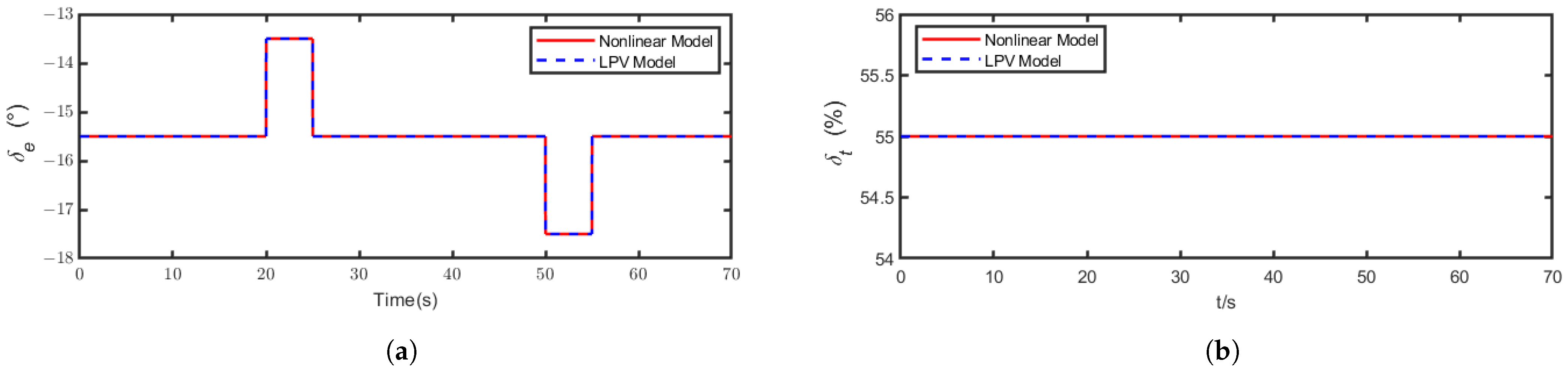
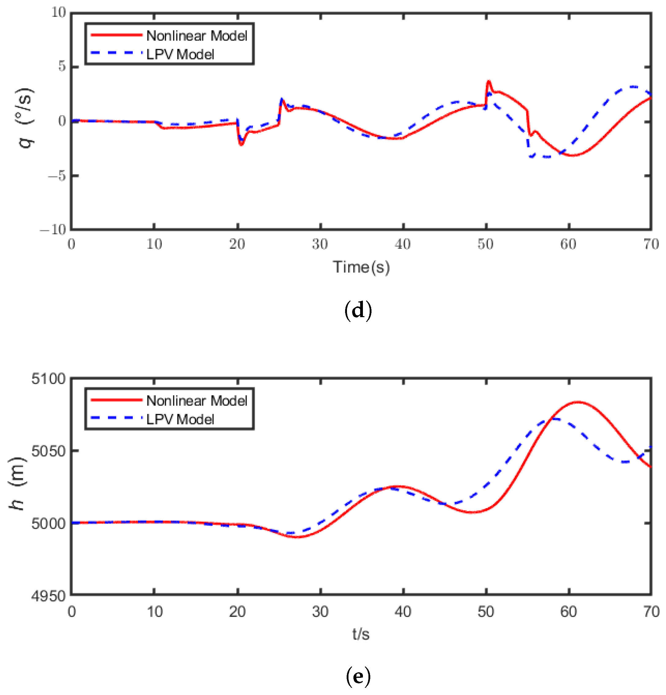
4.1. Mathematical Model Simulation

Since the LPV model is derived from the linearized small-disturbance model through interpolation and fitting operations, in order to verify whether the longitudinal LPV model for stable flight can effectively describe the nonlinear model’s dynamic characteristics and analyze the motion trends during morphing flight, a basic reference for subsequent controller design is provided. Therefore, a simulation verification process is designed in the numerical simulation section below.

Figure 3 shows the wingspan deformation of the longitudinal LPV model and the original longitudinal nonlinear dynamic model during the deformation simulation process. The red line in the figure represents the response curve of the nonlinear dynamic model, while the blue line represents the response curve of the LPV model. A scenario is designed where the same short-term control inputs and external disturbances are applied during the same wingspan deformation process. The variable-span aircraft is initially set to fly at a height of 5000 m and a speed of 40 m/s, with an initial wingspan morphing ratio of 0. At $t=10$ s, wingspan morphing begins, and the aircraft’s wingspan gradually transforms from the shortest (${\xi }_b=0$) to the longest (${\xi }_b=1$) by $t=40$ s, after which the wingspan morphing ratio remains constant. Additionally, during the morphing flight process, from $t=20$ to $t=25$ s and from $t=50$ to $t=55$ s, a +1° and −1° elevator deflections are added to the initial trim control. At the same time, a periodic disturbance is applied in the lift and drag directions starting at 30 s, with a disturbance period of 6.28 s and peak values of 50 N in each direction. A periodic disturbance of 50 N·m is also applied in the pitching moment direction.

The same elevator deflection and throttle opening are applied during the simulation, as shown in Figure 4. Figure 5 shows the simulation response of all system states.

As seen in Figure 5, in the case of applying the same elevator deflection angle and throttle setting, the flight states of the nonlinear dynamic model and the longitudinal LPV model of the morphing wing aircraft are very similar, with almost identical motion trends. Over time, both the angle of attack and pitch angle motion responses gradually diverge, causing the flight speed and altitude to deviate from the reference state designed by the LPV model, resulting in an accumulation of errors. This indicates that the open-loop control performance is not satisfactory, and a suitable controller needs to be added in the subsequent design. Overall, the LPV model still effectively describes the nonlinear model’s motion characteristics along the varying parameter trajectory and will be used as the benchmark model for the subsequent design.

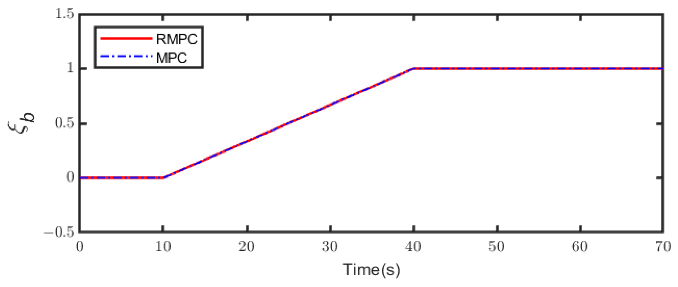
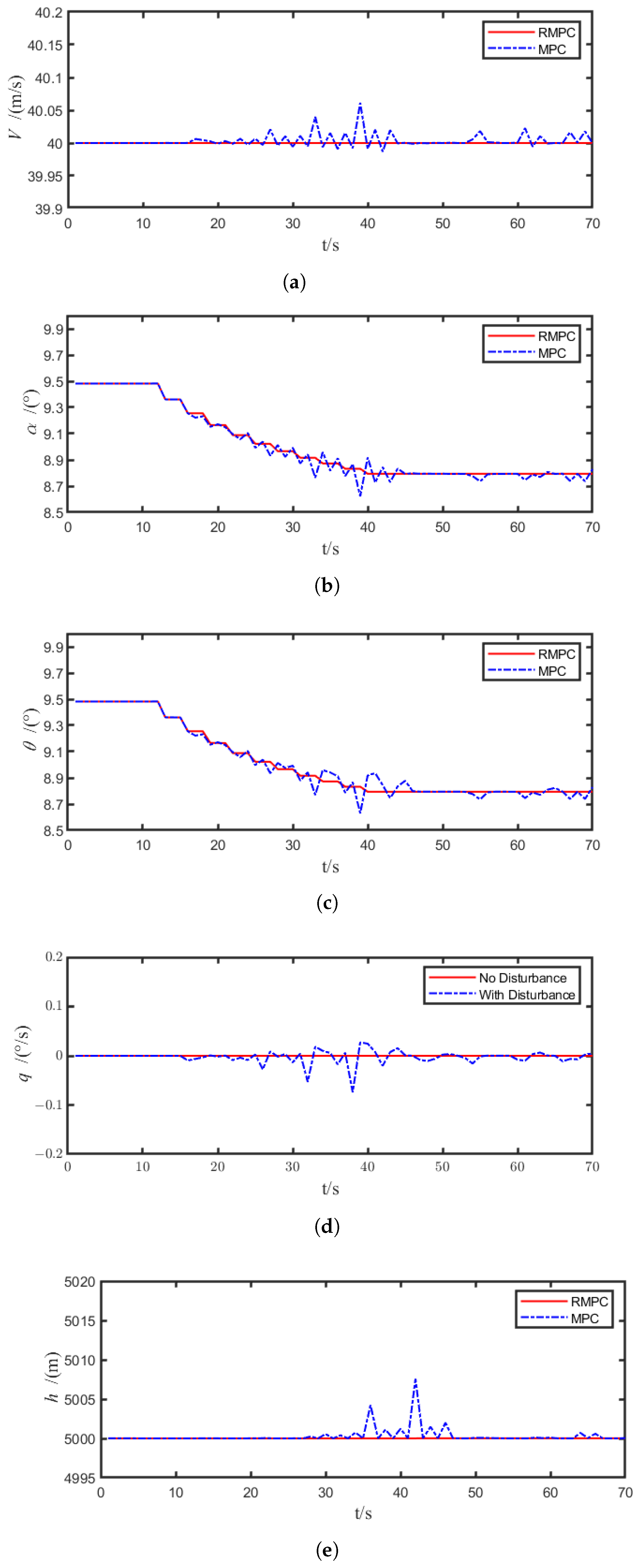
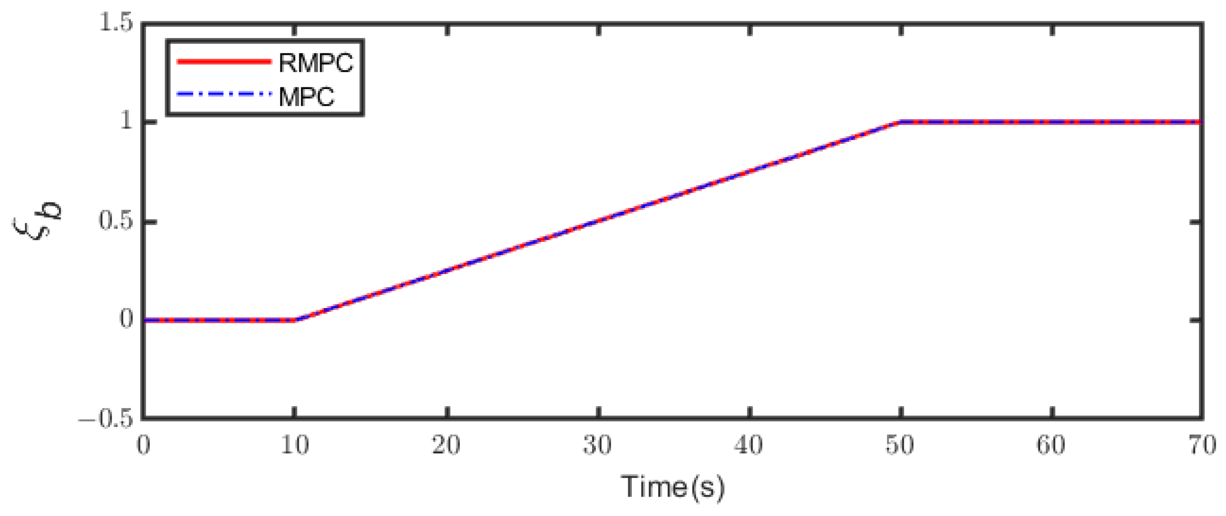
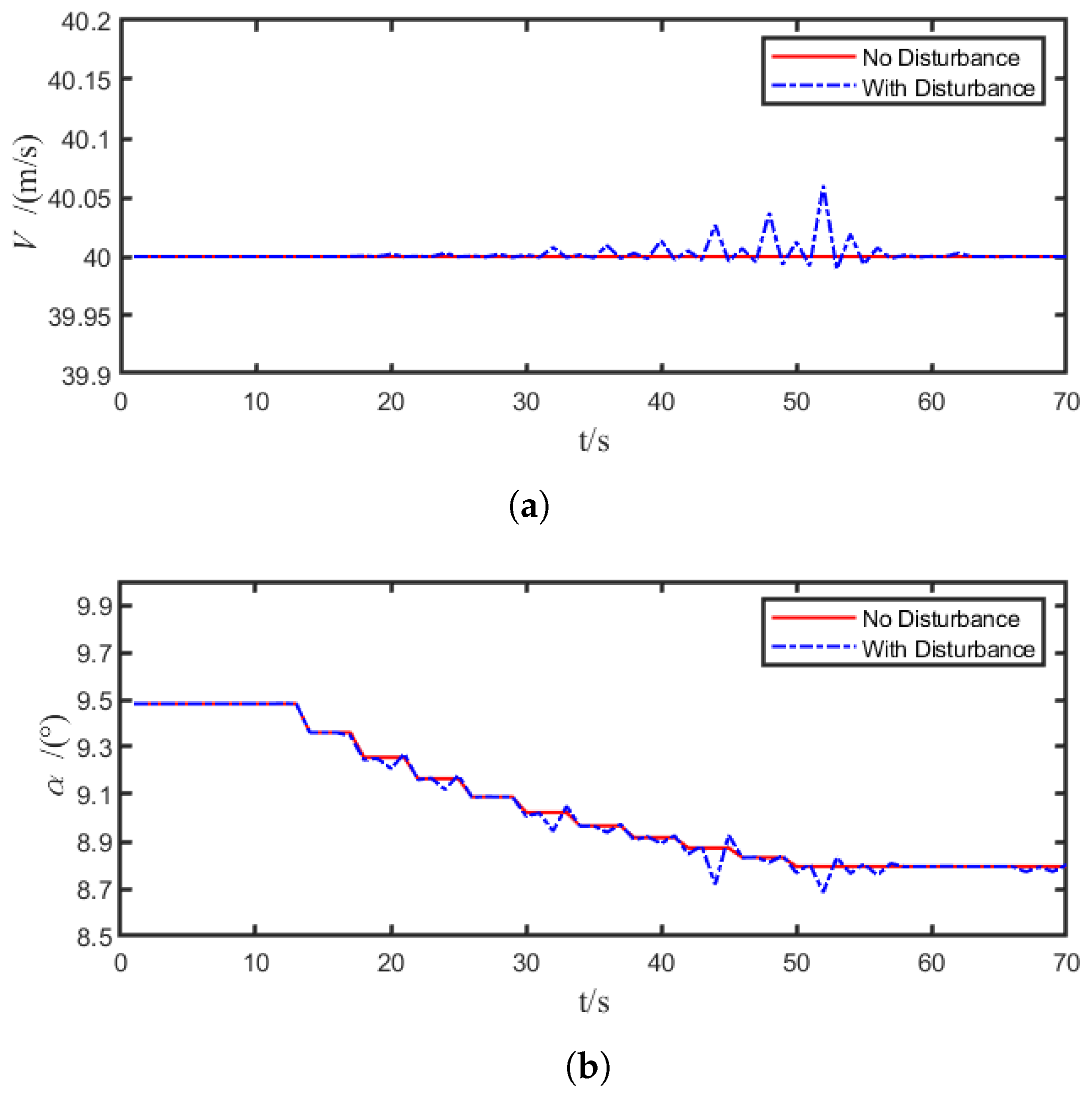
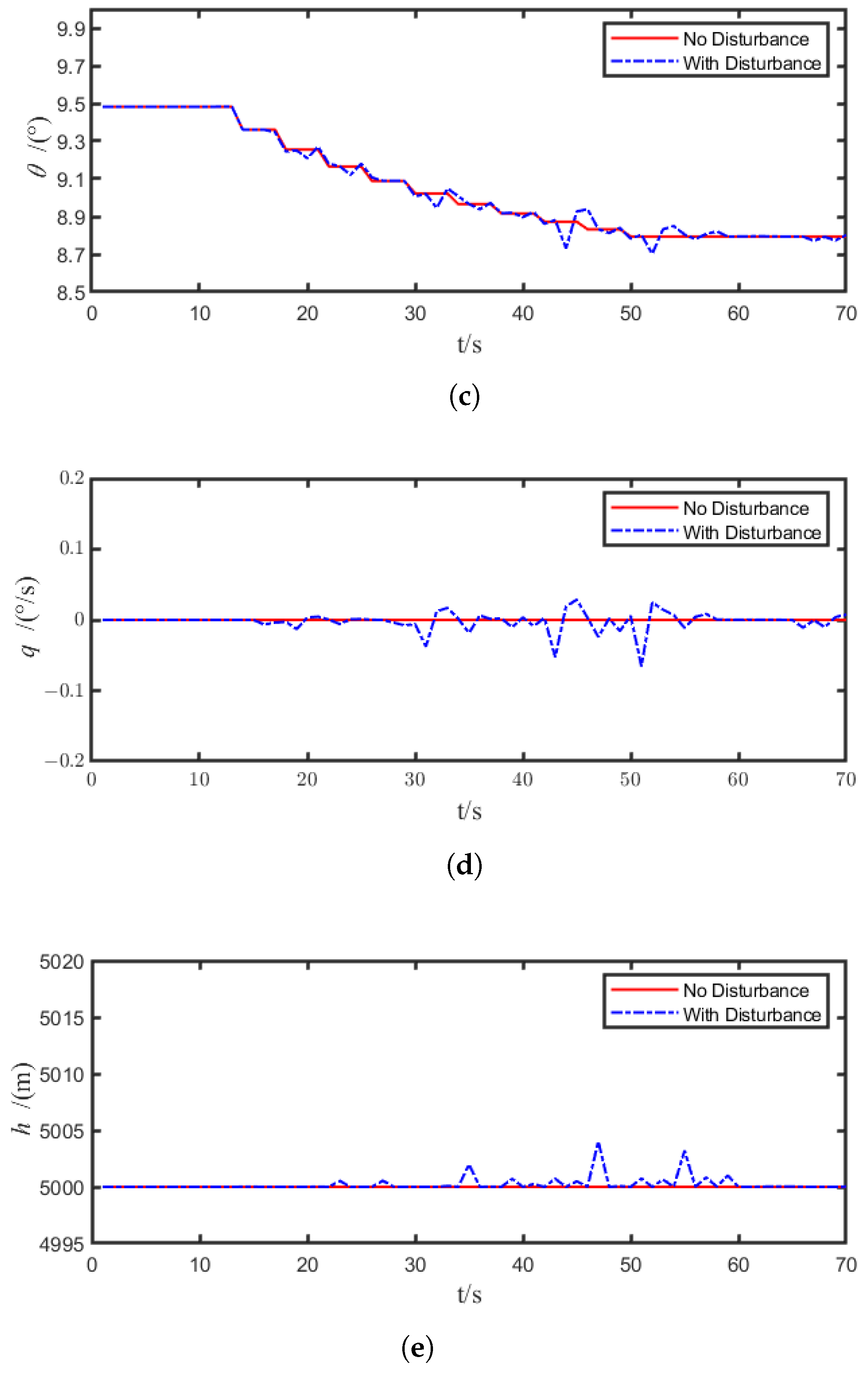
4.2. Controller Performance Verification

The control performance of the two model predictive controllers is validated through simulation. The following simulation experiment is designed: Initially, the wingspan morphing ratio is 0, and the variable-span aircraft is flying level at a height of 5000 m and a speed of 40 m/s. Starting from $t=10$ s, wingspan morphing begins, gradually increasing the wingspan morphing ratio. By $t=40$ s, the wingspan morphing ratio reaches 1, and remains constant thereafter. Periodic disturbances are applied simultaneously with the initiation of the wingspan deformation, with a disturbance period of 6.28 s and peak values of 100 N and 100 N·m for the disturbance force and moment, respectively, until the simulation ends at 70 s. Through calculation and testing, the design parameters of the MPC controller were determined. The selection of the control input weight matrix R needs to balance solvability and control performance. When R is chosen as the identity matrix, all control inputs are strictly constrained, which can lead to an unsolvable optimization problem. Therefore, the constraint on the second control input is relaxed. The state weight matrix Q should be greater than R, so that the system prioritizes optimizing the state rather than strictly controlling the input. When the terminal cost matrix S is large, the optimizer strongly constrains the terminal state, which may result in an unsolvable problem. Conversely, if S is too small, the optimization problem may become infeasible. To ensure that the controller remains solvable, constraint conditions are designed around the equilibrium points throughout the entire wingspan morphing process. The final weight matrices and constraint conditions are determined as follows:

$$\mathit{R}=\left[\begin{array}{cc}1& 0\\ 0& 0.01\end{array}\right],\mathit{Q}=\left[\begin{array}{ccccc}10& 0& 0& 0& 0\\ 0& 10& 0& 0& 0\\ 0& 0& 10& 0& 0\\ 0& 0& 0& 10& 0\\ 0& 0& 0& 0& 10\end{array}\right],\mathit{S}=\left[\begin{array}{ccccc}5& 0& 0& 0& 0\\ 0& 5& 0& 0& 0\\ 0& 0& 5& 0& 0\\ 0& 0& 0& 5& 0\\ 0& 0& 0& 0& 5\end{array}\right]$$

(45)

$${\mathit{u}}_{low}=\left[\begin{array}{c}{u}_{low1}\\ u_{low2}\end{array}\right]=\left[\begin{array}{c}-40\\ 0\end{array}\right],{\mathit{u}}_{high}=\left[\begin{array}{c}{u}_{high1}\\ u_{high2}\end{array}\right]=\left[\begin{array}{c}40\\ 100\end{array}\right]$$

(46)

$${\mathit{x}}_{low}=\left[\begin{array}{c}{x}_{low1}\\ x_{low2}\\ x_{low3}\\ x_{low4}\\ x_{low5}\end{array}\right]=\left[\begin{array}{c}0\\ -4\\ -10\\ -10\\ 0\end{array}\right],{\mathit{x}}_{high}=\left[\begin{array}{c}{x}_{high1}\\ x_{high2}\\ x_{high3}\\ x_{high4}\\ x_{high5}\end{array}\right]=\left[\begin{array}{c}60\\ 12\\ 15\\ 10\\ 5005\end{array}\right]$$

(47)

$$\mathit{\beta }={\left[\begin{array}{c}-u_{low1},-u_{low2},u_{high1},u_{high2},-x_{low1},-x_{low2},-x_{low3},-x_{low4},-x_{low5},x_{high1},x_{high2},x_{high3},x_{high4},x_{high5}\end{array}\right]}^T$$

(48)

Figure 6, Figure 7 and Figure 8 show that the red solid line represents the Robust Model Predictive Controller (RMPC), while the blue dashed line represents the MPC.The optimal control ${\mathit{U}}_{\left[k\right]}^{*}$ can be obtained through software, and the simulation control effect is shown by the red solid line in Figure 8.

When solving the RMPC, the wingspan deformation rate $\rho$ varies during this process. Therefore, the steady-state operating points of the parameter-varying system are determined based on Equations (9) and (10). To prevent the system from deviating beyond the controllable range and avoid overly tight or overly relaxed constraints leading to unsolvability or instability, constraints are selected near the equilibrium points to ensure that RMPC can always find a suitable control input under all possible wingspan variations.Taking ${\xi }_b=0$ as an example, the system’s state and input constraints are chosen as follows:

$$\left[\begin{array}{c}35\hfill \\ 9.0\hfill \\ 9.0\hfill \\ -0.6\hfill \\ 4995\hfill \end{array}\right]\le \left[\begin{array}{c}{v}_c\hfill \\ {\alpha }_c\hfill \\ {\theta }_c\hfill \\ q_c\hfill \\ h_c\hfill \end{array}\right]\le \left[\begin{array}{c}45\hfill \\ 9.7\hfill \\ 9.7\hfill \\ 0.6\hfill \\ 5005\hfill \end{array}\right],\left[\begin{array}{c}-16.0\hfill \\ 53.7\hfill \end{array}\right]\le \left[\begin{array}{c}{\delta }_e\hfill \\ {\delta }_t\hfill \end{array}\right]\le \left[\begin{array}{c}-15.0\hfill \\ 56.2\hfill \end{array}\right]$$

(49)

The boundary constraints of the disturbance force and disturbance moment are $\mid w_F\mid \le 100\mathrm{N}$ and $\left|w_M\right|\le 100\mathrm{N}/\left(\mathrm{m}\right)$. Under these disturbance constraints, the resulting terminal state set is as follows:

$$\Omega =\left\{(v,\alpha ,\theta ,q,h)\right|x_{min,\Omega }^i\le x^i\le x_{max,\Omega }^i\}$$

(50)

$$\left\{\begin{array}{c}{\mathit{x}}_{min,Omega}^i={[39.7,9.4,9.4,-0.1,4999.7]}^T\hfill \\ {\mathit{x}}_{max,\Omega }^i={[40.2,9.5,9.5,0.1,5001]}^T\hfill \end{array}\right.$$

(51)

Taking the prediction horizon as $N=10$, with a weighting coefficient of $\delta =3$, and a sampling time of $T_s=1$ s, the control effect is shown by the blue dashed line in Figure 8.

To test the robustness of the controller, a verification experiment is set, where the rate of deformation of the aircraft was reduced and the disturbance amplitude was increased. The wingspan deformation rate still changes from 0 to 1, and the deformation time period of the aircraft was extended from the original 10–40 s to 10–50 s. Periodic disturbances were introduced simultaneously with the wingspan deformation, with a disturbance period of 6.28 s and peak values of the disturbance force and disturbance moment increased from 100 to 120. The simulation results are shown in the figure below. Figure 9, Figure 10 and Figure 11 show that the red solid line represents the Robust Model Predictive Controller (RMPC), while the blue dashed line represents the MPC.

The true results show that when the wingspan is low and system disturbances are considered, the Model Predictive Controller (MPC) can effectively adjust during the deformation process of the variable-wingspan aircraft. It adjusts the control inputs in time to achieve stable flight. However, as the wingspan increases, the flight speed and altitude deviate from the initial state to some extent, and there are oscillations in the attitude angle. This indicates that the designed MPC has good control performance when system disturbances are not considered but has poor disturbance rejection capability. By observing the robust model predictive controller, and comparing the control performance under different deformation rates and disturbance amplitudes, it can be found that when the wingspan deformation rate is relatively small and subject to composite disturbances, the robust predictive control exhibits good control performance. It can quickly implement regulatory control, with system states fluctuating within a small range, ensuring the stable flight of the morphing aircraft. As the wingspan deformation rate increases, the impact of disturbances on the system reaches its peak. However, under the action of the robust controller, the disturbances are effectively suppressed, allowing the morphing aircraft to respond quickly to various commands and achieve stable flight. This demonstrates that the designed RMPC ensures the robustness and global stability of the morphing flight process of the morphing aircraft.

5. Conclusions

When wingspan deformation is small and system disturbances are considered, the model predictive controller (MPC) can effectively adjust the control inputs during the morphing process of the aircraft, enabling stable flight. However, as wingspan deformation increases, the flight speed and altitude deviate to a certain extent from the initial state, and oscillations appear in the attitude angles. This indicates that the designed MPC performs well in terms of control when system disturbances are not considered, but it has poor disturbance rejection capability.

Observing the robust model predictive controller (RMPC), by comparing the control performance under different deformation rates and disturbance amplitudes, it can be seen that when the wingspan deformation is small and composite disturbances exist, RMPC exhibits better control performance. It can quickly implement regulatory control, keeping system states fluctuating within a small range, thereby ensuring the stable flight of the morphing aircraft. As wingspan deformation increases, the effect of disturbances on the system reaches its maximum. However, under the action of the robust controller, the disturbances are effectively suppressed. Even in different disturbance environments, the morphing aircraft can still respond quickly to various commands and achieve stable flight. This demonstrates that the designed RMPC ensures the robustness and global stability of the morphing flight process.

References

1. Guo, T.; Zhu, C.; Feng, L.; Duan, Y.; Chen, H. Aerodynamic-driven morphing aircraft and its aerodynamic design. Chin. J. Aeronaut. 2024, 37, 103377. [Google Scholar] [CrossRef]
2. Yang, T.; Zhang, X.; Wu, L.; Ai, J. Flight Dynamic Modeling and Control for a Telescopic Wing Morphing Aircraft via Asymmetric Wing Morphing. Aerosp. Sci. Technol. 2017, 70, 328–338. [Google Scholar] [CrossRef]
3. Guo, T.; Zhu, C.; Feng, L.; Duan, Y.; Chen, H. Aerodynamic-driven morphing aircraft and its overall design. Chin. J. Aeronaut. 2024, 38, 103322. [Google Scholar] [CrossRef]
4. Chu, L.; Li, Q.; Gu, F.; Du, X.; He, Y.; Du, Y. Design, Modeling, and Control of Morphing Aircraft: A Review. Chin. J. Aeronaut. 2022, 35, 220–246. [Google Scholar] [CrossRef]
5. Pazooki, M.S.; Pazooki, J.S.; Moghadasi, R.; Ahmadi, M.; Amini, D.; Zekri, Y.; Friswell, M.I. A Review of Control Strategies Used for Morphing Aircraft Applications. Chin. J. Aeronaut. 2024, 37, 436–463. [Google Scholar] [CrossRef]
6. Weisshaar, T.A. Morphing Aircraft Systems: Historical Perspectives and Future Challenges. J. Aircr. 2013, 50, 337–353. [Google Scholar] [CrossRef]
7. Yuan, L.; Wang, L.; Xu, J. Adaptive Fault-Tolerant Controller for Morphing Aircraft Based on the L2 Gain and a Neural Network. Aerosp. Sci. Technol. 2023, 132, 107985. [Google Scholar] [CrossRef]
8. Wang, S.; Chao, T.; Han, Y.; Du, H. Research Progress on Morphing Aircraft Morphing Strategies and Control Methods. Tactical Missile Technol. 2024, 4, 1–15. [Google Scholar] [CrossRef]
9. Yin, M.; Lu, Y.; He, Z. LPV Modeling and Robust Gain-Scheduling Control of Morphing Aircraft. J. Nanjing Univ. Aeronaut. Astronaut. 2013, 45, 202–208. [Google Scholar] [CrossRef]
10. Yang, Q.; Hu, L.; Zhang, Y.; Lü, X.; Li, X.; Cai, G. Attitude Control of Morphing Aircraft Based on Uncertain LPV System. J. Ordnance Equip. Eng. 2023, 44, 127–133. [Google Scholar]
11. Wu, Q.; Liu, Z.; Ding, B.; Zhu, L. Design of Sliding Mode Controller with Self-adaption for a Morphing Aircraft. In Proceedings of the 2018 Chinese Automation Congress (CAC), Xi’an, China, 30 November–2 December 2018; pp. 122–127. [Google Scholar] [CrossRef]
12. Athayde, A.; Moutinho, A.; Azinheira, J.R. Experimental Nonlinear and Incremental Control Stabilization of a Tail-Sitter UAV with Hardware-in-the-Loop Validation. Robotics 2024, 13, 51. [Google Scholar] [CrossRef]
13. Yin, M. Research on Coordinated Control of Morphing and Flight for Morphing Aircraft. J. Aircr. Control 2016. [Google Scholar]
14. Zhao, M.; Li, S. Switched Robust Predictive Control for Constrained Nonlinear Systems. Control Theory Appl. 2010, 27, 4–495. [Google Scholar]
15. Zanon, M.N.; Mandić, D.R.; Domahidi, A.; Morari, M.; Jones, C.N. On Real-Time Robust Model Predictive Control. Automatica 2014, 50, 683–694. [Google Scholar] [CrossRef]
16. Xu, W.; Li, Y.; Pei, B.; Yu, Z. Coordinated Optimization Control of Morphing Aircraft Based on Multi-Model MPC. Syst. Eng. Electron. 2023, 45, 2902–2911. [Google Scholar]
17. Shao, P.; Dong, Y.; Li, J.; Qu, G. Model Predictive Control Method for a Foldable-Wing Biomimetic Morphing UAV Based on an LPV System. J. Xi’an Aeronaut. Univ. 2020, 38, 3–10. [Google Scholar]
18. Koehler, J.; Soloperto, R.; Müller, M.A.; Allgöwer, F. A Computationally Efficient Robust Model Predictive Control Framework for Uncertain Nonlinear Systems. IEEE Trans. Autom. Control 2021, 66, 794–801. [Google Scholar] [CrossRef]
19. Lin, X.; Görges, D. Robust Model Predictive Control of Linear Systems with Predictable Disturbance with Application to Multiobjective Adaptive Cruise Control. IEEE Trans. Control Syst. Technol. 2019, 28, 1460–1475. [Google Scholar] [CrossRef]
20. Wang, E.; Lu, H.; Zhang, J.; Wang, C.; Qiao, J. A Novel Adaptive Coordinated Tracking Control Scheme for a Morphing Aircraft with Telescopic Wings. Chin. J. Aeronaut. 2024, 37, 148–162. [Google Scholar] [CrossRef]
21. Chen, S.; Jia, M.; Liu, Y.; Gao, Z.; Xiang, X. Deformation modes and key technologies of aerodynamic layout design for morphing aircraft: Review. Acta Aeronaut. Astronaut. Sin. 2024, 45, 629595. [Google Scholar] [CrossRef]
22. Xu, W.; Li, Y.; Pei, B.; Yu, Z. Coordinated Intelligent Control of the Flight Control System and Shape Change of Variable Sweep Morphing Aircraft Based on Dueling-DQN. Aerosp. Sci. Technol. 2022, 130, 107898. [Google Scholar] [CrossRef]
23. Cai, G.; Yang, Q.; Mu, C.; Li, X. Design of Linear Parameter-Varying Controller for Morphing Aircraft Using Inexact Scheduling Parameters. IET Control Theory Appl. 2023, 17, 493–503. [Google Scholar] [CrossRef]
24. González Cisneros, P.S.; Werner, H. Nonlinear Model Predictive Control for Models in Quasi-Linear Parameter Varying Form. Int. J. Robust Nonlinear Control 2020, 30, 3945–3959. [Google Scholar] [CrossRef]
25. Ge, J.; Guo, J.; Wang, H.; Zhang, B.; Wan, Y.; Tang, S. Hypersonic Morphing Aircraft Adaptive Model Predictive Control. J. Beijing Univ. Aeronaut. Astronaut. 2024, 1–19. [Google Scholar] [CrossRef]
26. Minniti, M.V.; Grandia, R.; Farshidian, F.; Hutter, M. Adaptive CLF-MPC with Application to Quadrupedal Robots. IEEE Robot. Autom. Lett. 2022, 7, 565–572. [Google Scholar] [CrossRef]
27. Shao, P.; Dong, Y.; Ma, S. Model Predictive Control Based on Linear Parameter-Varying Model for a Bio-Inspired Morphing Wing UAV. In Proceedings of the 2021 International Conference on Robotics and Control Engineering, Beijing, China, 16–18 April 2021; pp. 59–63. [Google Scholar] [CrossRef]
28. Limon, D.; Bravo, J.M.; Alamo, T.; Camacho, E.F. Robust MPC of Constrained Nonlinear Systems Based on Interval Arithmetic. IEE Proc.-Control Theory Appl. 2005, 152, 325–332. [Google Scholar] [CrossRef]
29. Santos, T.L.M.; Cunha, V.M. Robust MPC for Linear Systems with Bounded Disturbances Based on Admissible Equilibria Sets. Int. J. Robust Nonlinear Control 2021, 31, 2690–2711. [Google Scholar] [CrossRef]
30. Liu, Z.; Ozay, N. On the Convergence of the Backward Reachable Sets of Robust Controlled Invariant Sets for Discrete-Time Linear Systems. In Proceedings of the 2022 IEEE 61st Conference on Decision and Control (CDC), Cancun, Mexico, 6–9 December 2022; pp. 4270–4275. [Google Scholar] [CrossRef]
Figure 1. Schematic diagram of wingspan morphing for a variable-span aircraft.
Applsci 15 04380 g001
Figure 2. This illustrates the relationship between longitudinal aerodynamic coefficients and angle of attack under different wingspan deformation rates for a morphing wing aircraft at an altitude of 5000 m and a Mach number of Ma = 0.12 . (a), (b), and (c), respectively, describe the relationships between the pitch angle and the lift coefficient, drag coefficient, and pitching moment coefficient.
Applsci 15 04380 g002
Figure 3. Wingspan morphing ratio during simulation verification process.
Applsci 15 04380 g003
Figure 4. Input variable values during the simulation verification process: (a) elevator angle, and (b) throttle setting.
Applsci 15 04380 g004
Figure 5. Flight response curves during the morphing process in the simulation verification process: (a) flight speed, (b) angle of attack, (c) pitch angle, (d) pitch rate, and (e) flight altitude.
Applsci 15 04380 g005aApplsci 15 04380 g005b
Figure 6. Wing span morphing ratio during the controller performance verification.
Applsci 15 04380 g006
Figure 7. Input variable values during the controller performance verification: (a) elevator angle, and (b) throttle setting.
Applsci 15 04380 g007
Figure 8. Flight response curves during the morphing process in the controller performance verification: (a) flight speed, (b) angle of attack, (c) pitch angle, (d) pitch rate, and (e) flight altitude.
Applsci 15 04380 g008
Figure 9. Verification experiment for the wingspan morphing ratio during the controller performance verification.
Applsci 15 04380 g009
Figure 10. Verification experiment for the input variable values during the controller performance verification: (a) elevator angle, and (b) throttle setting.
Applsci 15 04380 g010
Figure 11. Verification experiment flight response curves during the morphing process in the controller performance verification: (a) flight speed, (b) angle of attack, (c) pitch angle, (d) pitch rate, and (e) flight altitude.
Applsci 15 04380 g011aApplsci 15 04380 g011b
Disclaimer/Publisher’s Note: The statements, opinions and data contained in all publications are solely those of the individual author(s) and contributor(s) and not of MDPI and/or the editor(s). MDPI and/or the editor(s) disclaim responsibility for any injury to people or property resulting from any ideas, methods, instructions or products referred to in the content.