Abstract
As the population continues to grow, the need for increased food production has become increasingly evident. However, the agricultural workforce is decreasing due to industrialization. To address this gap, numerous research efforts are underway to adopt robots for harvesting. While significant progress has been made, especially in fruit harvesting using robotic systems, there are still inefficiencies and areas where human intervention is necessary. This paper proposes an algorithm for selecting the position of a mobile manipulator for fruit harvesting using an inverse reachability map to achieve automation and enhance efficiency. Additionally, a method for collision-free path planning in joint space using the model predictive artificial potential field (MPAPF) algorithm is proposed. The effectiveness of the proposed position selection and path planning algorithms was validated through harvesting simulations and a collision-free path was validated in experiments.
1. Introduction
With the continuous increase in the global population, food production must also be increased. However, modern society is facing challenges in food production due to the decline in the agricultural workforce caused by industrialization. To address these issues, agricultural automation technology is advancing and innovations in the field of harvesting robots are expected to contribute to improving global food productivity [1,2,3].
Fruit harvesting with robots requires the precise identification of tree and target fruit locations. However, the irregular growth patterns of trees and fruits make them difficult to detect. Furthermore, it is crucial to avoid damaging branches or other harvestable items during the harvesting process. Fruit harvesting using robotic systems requires a computer vision system to detect target objects and the surrounding environment, along with a harvesting method for the manipulator that avoids causing damage to other parts of the tree [4]. To address these challenges, significant research has been conducted. Related works are roughly divided into two main areas: computer vision systems for detecting target fruits and obstacles, and collision-free path planning for the robotic manipulator to avoid damaging fruits and trees.
In robotic fruit harvesting, RGB-D cameras or Lidar sensors are mainly used. RGB-D cameras are commonly used for fruit recognition based on color information or for measuring the position of fruits [5,6,7,8,9]. Although RGB-D cameras are sensitive to surrounding lighting conditions, their advantages in cost and computational efficiency make them suitable for practical applications in agriculture [10]. For overall mapping of orchards or precise fruit shape measurements, Lidar is used [11,12,13,14,15,16,17]. High costs made it difficult to use in agriculture in the past, but advancements have made it more affordable and accessible. To overcome individual limitations and enhance overall accuracy, research that integrates multiple vision systems is underway.
Trees grow randomly in nature, and fruits typically cluster together. Because of these characteristics, a harvesting robot may collide with tree branches and nearby fruits. Therefore, it is crucial to consider the surrounding environment when generating robot paths to minimize damage to the tree, its branches, and nearby fruits during harvesting. Commonly used path planning algorithms for robot arm include the A*, rapidly exploring random tree (RRT) and artificial potential field (APF) algorithms. The A* algorithm has the advantage of reaching the destination while avoiding obstacles and finding the shortest path, but it has a drawback in that generating paths in three-dimensional space becomes computationally expensive due to an excessive number of grid points [18].
RRT generates paths by growing a tree through random sampling, leading to non-smooth paths and detours in three-dimensional spaces. The branches that are extended from detours can lead to inefficiency in path planning or computation time. The efficiency of path generation directly impacts the operational efficiency of harvesting robots. Thus, it requires modification to minimize computation time. An algorithm called AtBi-RRT was proposed in [19], based on the Bi-RRT algorithm [20], to accelerate path decision speed by simultaneously growing trees from the initial and the target positions, along with the application of a target gravity concept and an adaptive parameter adjustment method. The proposed algorithm was used in collision-free motion for a litchi-picking robot, with improved planning time. Another algorithm called tGSRT, incorporating the concept of target gravity for increased speed and a GA for path optimization, was proposed in [21] for litchi-picking robot path planning.
APF offers the advantages of simplicity and high speed computation, but it easily stuck in local minima and has oscillations in the generated paths. An algorithm called TO-RRT was proposed in [22], combining RRT and APF, utilizing a node-first search strategy to prevent the local minima problems caused by APF and employing the regression superposition algorithm to minimize computation time. The proposed algorithm was used for a citrus-picking robot. In [23], the IAPF was proposed, which is based on an artificial potential function incorporated with a sigmoid function element to avoid local minima.
Despite various developments in orchard mapping, fruit detection, path planning and automated systems over the past 30 years, currently developed harvesting robots are considered less practical than manual harvesting in most applications [24]. Significant research has been conducted on fruit harvesting robots; however, the question of where a harvesting robot should be positioned to efficiently harvest a fruit or a cluster of fruits has been overlooked. In [25], a fully integrated system was implemented for autonomous citrus harvesting, but positioning it for harvesting specific target fruits still relied on manual intervention. The positioning of harvesting robots has not been sufficiently studied, as it often relies on manual placement by humans [26], is constrained by pre-defined and highly structured environments, such as planar orchards [27], or excludes target fruits that are inaccessible due to fixed robot bases locations and limited approach angles [28]. Placing robots in appropriate positions not only reduces the risk of harvesting failure and collisions with obstacles but also shortens path generation time [29]. Furthermore, it is inefficient to move the entire robot each time harvesting takes place, in contrast to manipulating the harvest from a fixed position [30]. The efficiency of the harvesting process can be increased by maximizing the number of fruits harvested from a single location with arm motions alone.
This paper proposes a new approach to selecting an optimal position of a harvesting robot and the orientation of end-effector for harvesting multiple fruits based on an inverse reachability map. Pre-determining the position of the mobile manipulator and the orientation of the end-effector enables efficient harvesting of as many fruits as possible from a single position, without the need to move the entire system. With the proposed scheme, the success rate of harvesting can be increased, since it takes into account the manipulator workspace and obstacles in advance.
This paper also proposes an algorithm for collision-free path planning for robot systems called the model predictive artificial potential field (MPAPF). Typically, path planning for a manipulator using APF involves calculating the gradient of the potential function acting on the end-effector and computing the torques applied to each joint using the manipulator Jacobian matrix. Alternatively, a grid-based method is employed, moving the end-effector to the point with the lowest potential value in the vicinity. These methods have a limitation in that it is difficult to account for the manipulator workspace or joint limits because the path planning is performed in the end-effector space. In MPAPF, by planning the path in joint space, singularities can be avoided and joint limits can be easily considered. Furthermore, the potential field is formed for multiple points on the manipulator, so MPAPF can avoid collisions between the entire manipulator and obstacles. Additionally, the risk of falling into a local minimum is reduced due to the complexity of the potential field. The positioning and path planning assumes that the locations of the tree and fruit are known in advance. The entire harvesting process was implemented in a simulator with a model of an orchard, and collision-free paths in complex environments were verified in experiments. The main contributions of this paper as follows:
- A new method to select the position of the robot base and the orientation for approaching a target fruit of the end-effector is proposed for increased efficiency and reduced risk of failure in harvesting.
- A novel joint-space collision-free path planning method, the model predictive artificial potential field (MPAPF), is proposed to avoid singularity and to consider the joint limits and geometry of the manipulator. By optimizing potential values over multiple steps, it also reduces the risk of local minima.
The remainder of this paper is structured as follows: Section 2 covers the method of selecting a position using the inverse reachability map. Section 3 explains the collision-free path planning method using the MPAPF algorithm. Section 4 validates the algorithm with applications in harvesting simulations. Section 5 demonstrates experiments with collision-free paths and the conclusions are provided in Section 6.
2. Position and Orientation Selection
2.1. Reachability Map
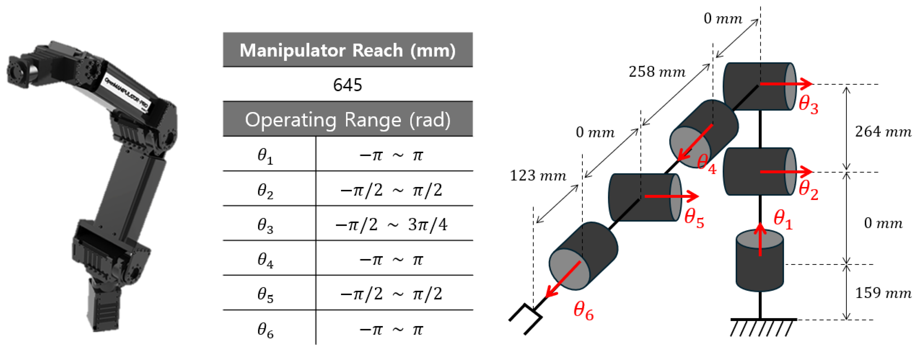
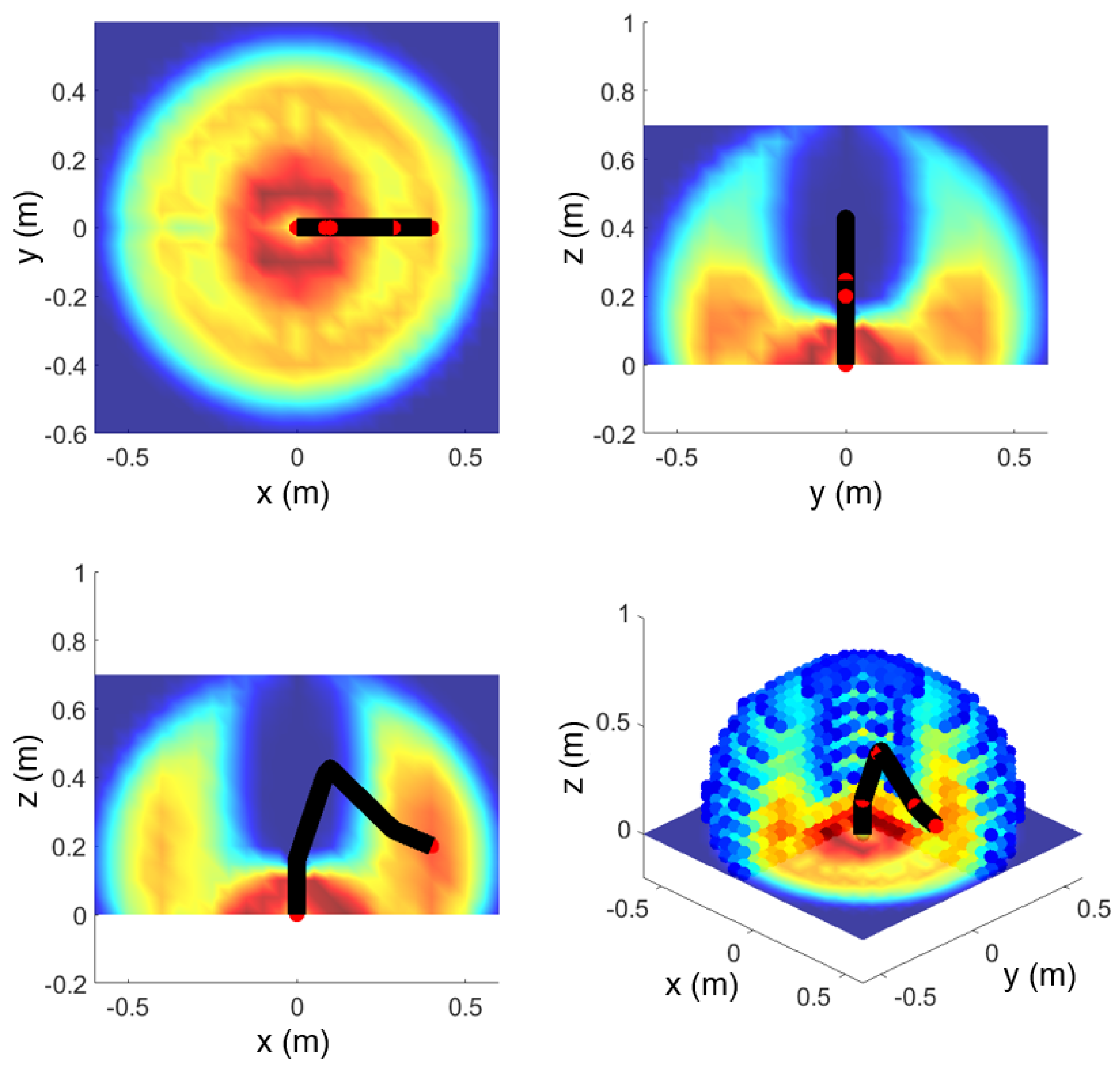
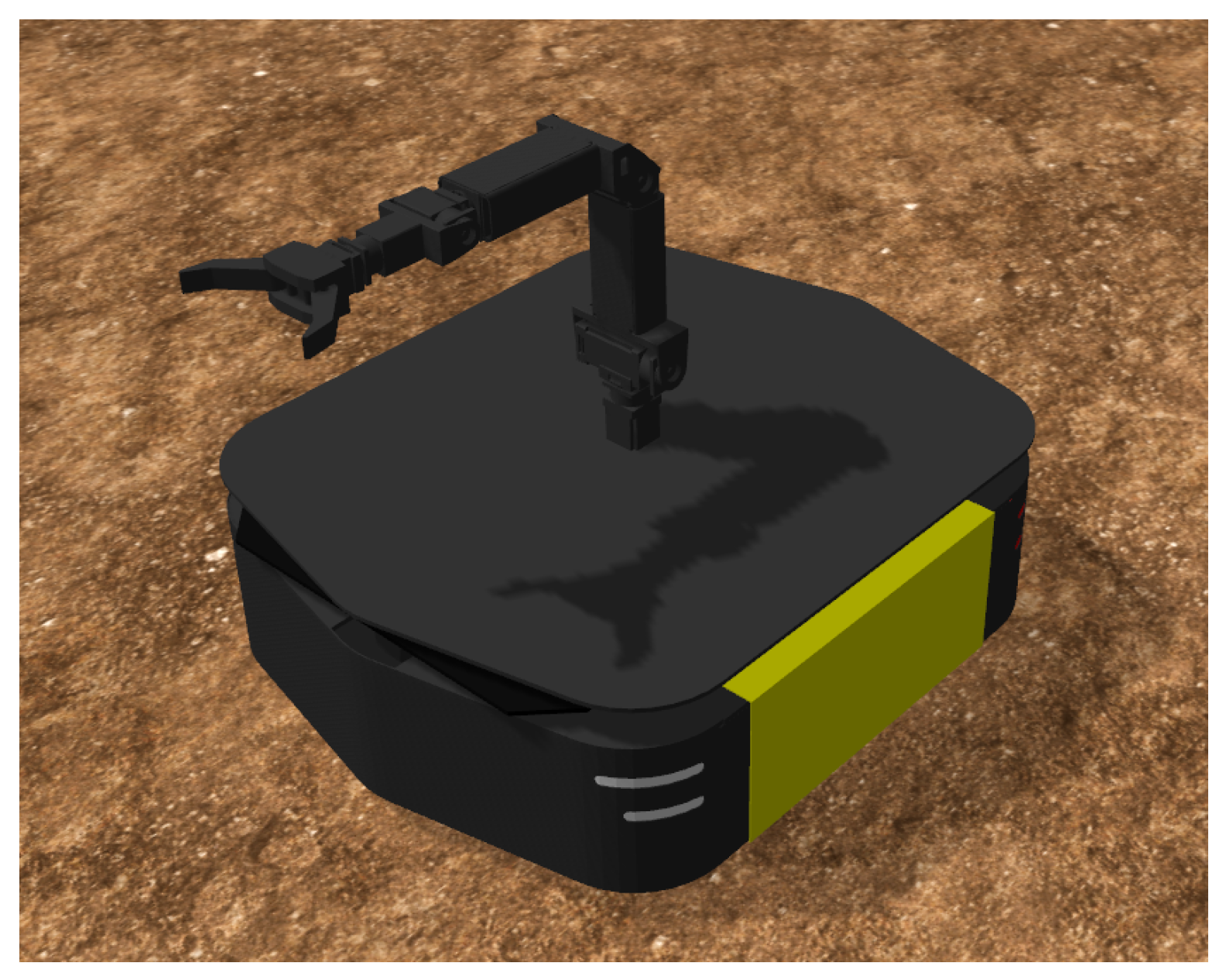
The reachability map was generated by voxelizing the space and solving the inverse kinematics for all orientations where the end-effector can approach the respective voxel, adding up the reachability scores only when solutions within the joint limits exist. A pseudo-code for computing a reachability map is shown in Algorithm 1. The reachability map for a manipulator—Open-Manipulator Pro, manufactured by Robotis (shown in Figure 1)—is depicted in Figure 2, where red and blue respectively represent the maximum and the minimum values of the reachability score, with yellow in the middle. The space was voxelized using a grid size of 50 mm, covering 1.4(W) × 1.4(D) × 0.7(H) in meters, since the manipulator reach is 645 mm. The orientation for approaching the voxels was set to spacing for each axis within the range of to .
| Algorithm 1 Reachability Map Construction |
|
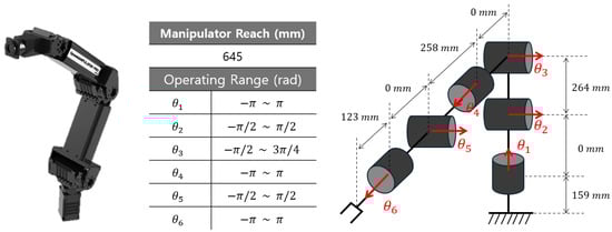
Figure 1.
Open−Manipulator Pro used in this work and its specification.
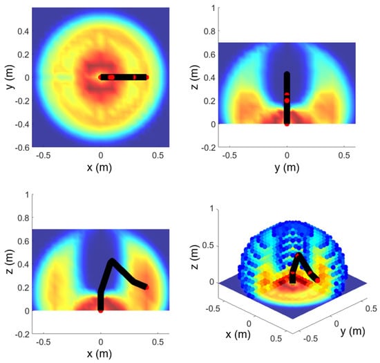
Figure 2.
Reachability map of Open−Manipulator Pro. Red and blue respectively represent the maximum and the minimum values of the reachability score, with yellow in the middle.
A reachability map is a collection of where and denote the positions of the end-effector and the manipulator base, respectively. denotes the manipulator workspace and denotes the manipulability, an indicator on how easily the manipulator moves in all directions. In this work, the one proposed in [31] is used:
where and denote the minimum and the maximum eigenvalues and denotes the manipulator Jacobian at joint angle , with the inverse kinematics .
2.2. Inverse Reachability Map
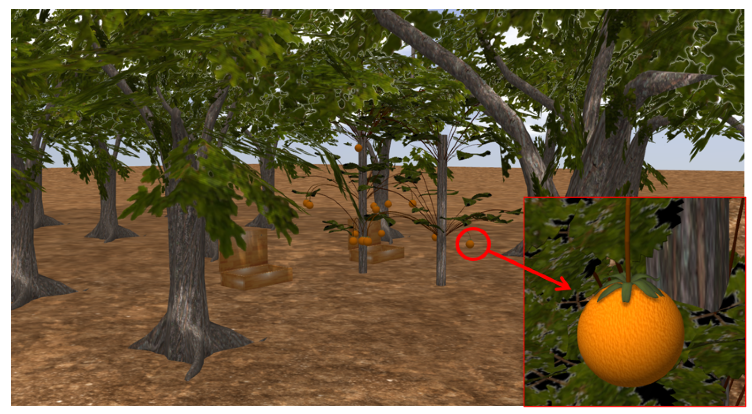
While the reachability map shows the reachable area of the end-effector with a fixed robot base, the inverse reachability map demonstrates where to position the robot base so that the end-effector can reach a specific target point. The target fruits focused in this paper are Kanpei, a citrus cultivar, which are cultivated by suspending them separately on support structures during growth to prevent them from falling due to their weight or branches breaking, as shown in Figure 3. Since their pedicels grow upward, the roll and pitch angles of the end-effector of the harvesting robot are assumed to be zero. In addition, because the robot base cannot be lifted up and down, it is assumed that its vertical coordinate is also zero.
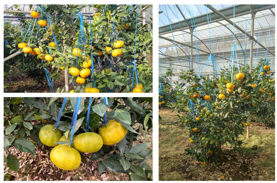
Figure 3.
Kanpei cultivation environment.
Similar to generating the reachability map, the inverse reachability map is generated by voxelizing the space and varying the yaw angle of the end-effector position while solving the inverse kinematics. If the obtained joint angles satisfy the joint limits, the forward kinematics is solved using the obtained inverse kinematics solution to calculate the positions of the joints and check for collisions between the manipulator and obstacles. If there are no collisions, the manipulability score is calculated and stored. The same procedure is repeated for multiple targets, voxelizing the space around the centroid of the location of each target in a similar manner. Directly summing the individual maps could lead to issues where certain positions might have the highest score, despite there being no feasible solution for some fruit. To mitigate this, we assign negative values to positions where no solution exists and utilize the summed inverse reachability scores. If there is no common solution, different positions were selected for fruits. A pseudo-code for computing an inverse reachability map is shown in Algorithm 2. Once positions are determined, the end-effector orientation is selected with the highest single reachability score by varying the approach angle to the target location.
| Algorithm 2 Inverse Reachability Map Construction |
|
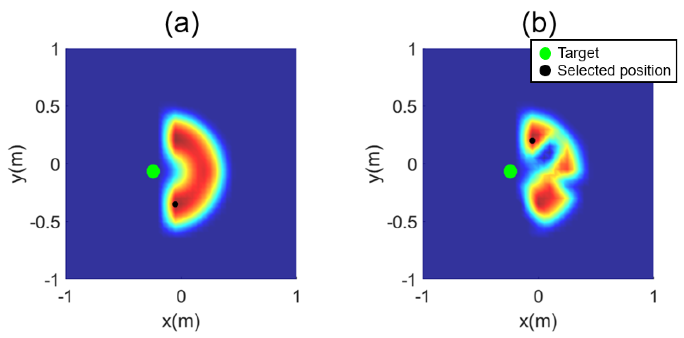
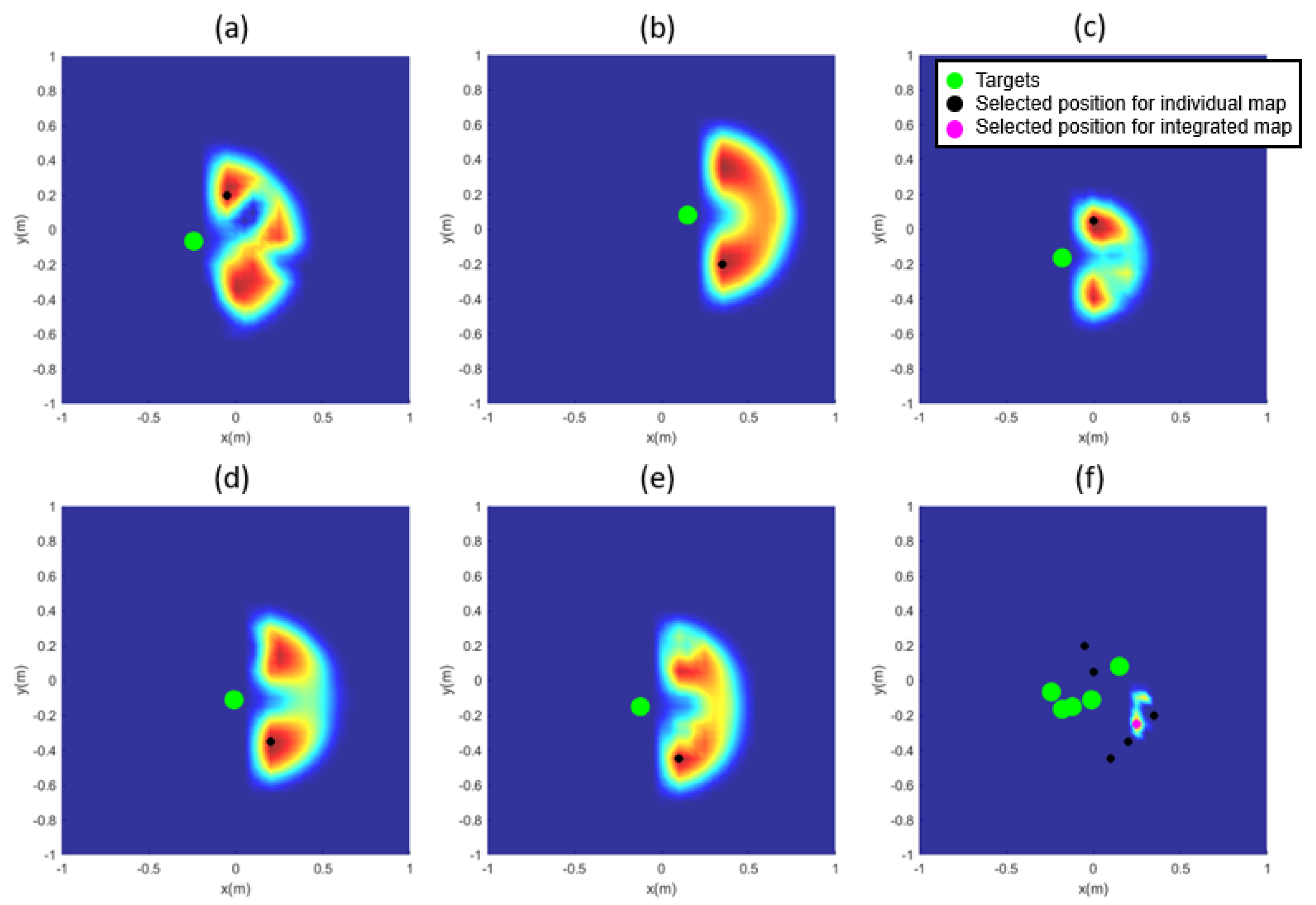
Figure 4 depicts an example of an inverse reachability map for a random target. When there are no obstacles for the same target fruit, the map appears symmetrically, as shown in Figure 4a. However, when obstacles exist, the IRM appears restricted, as shown in Figure 4b. The target fruit is depicted as a green circle, and the position with the highest score is marked with a black circle, where red and blue respectively represent the maximum and the minimum values of the inverse reachability score, with yellow in the middle. Examples of the map for 15 obstacles and five target fruits are presented in Figure 5. The space was voxelized using a grid size of 50 mm, with the centroid of the targets as its center. Voxelized space spans 1.4(W) × 1.4(D) in meters. The orientation for approaching a target fruit of the end-effector ranges from to , with a grid size of radians.
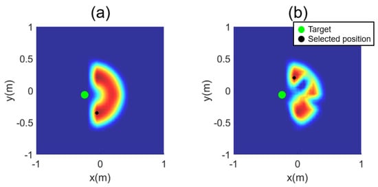
Figure 4.
Inverse reachability map: (a) without obstacles; (b) with obstacles.
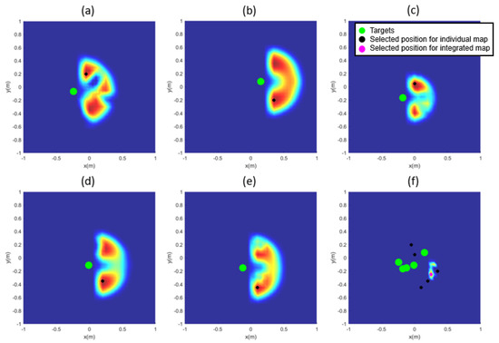
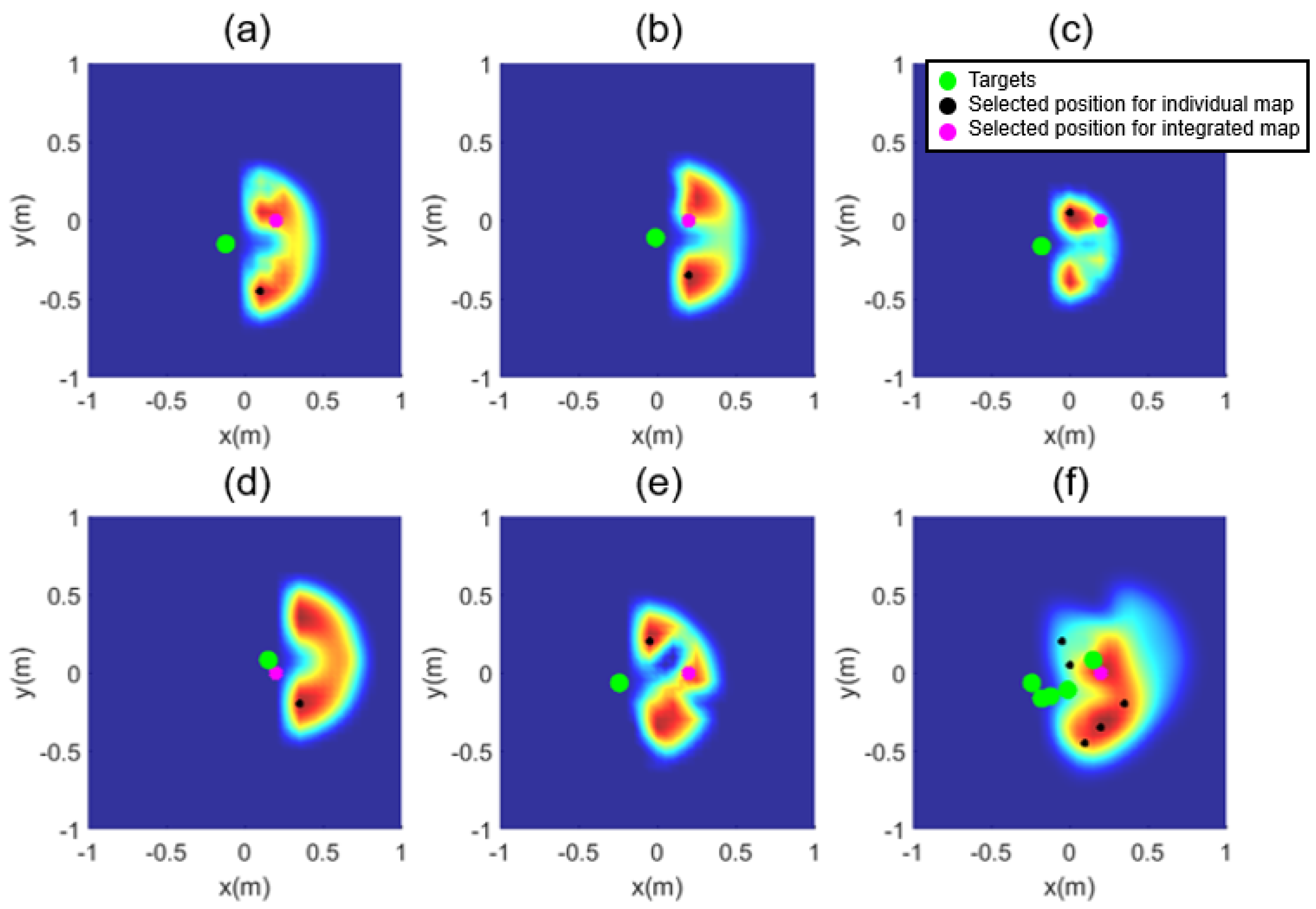
Figure 5.
Inverse reachability map: (a–e) for each target and (f) for the aggregate target.
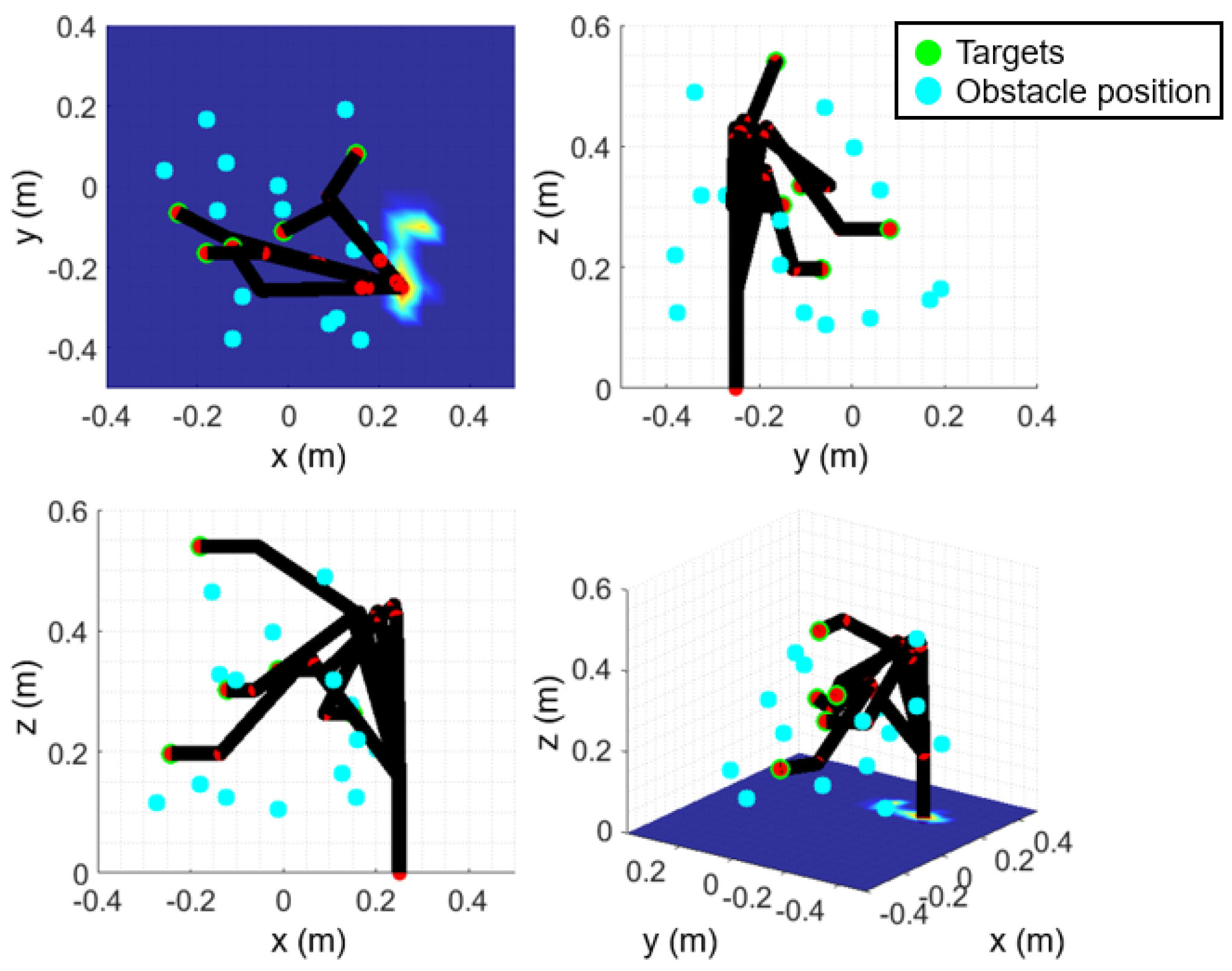
Figure 5a–e represent an inverse reachability map for each of the five target fruits, and Figure 5f shows the integrated inverse reachability map for all the five target fruits. The target fruits are depicted as green circles, and the positions with the highest score in individual maps are marked with black circles. In Figure 5f, the magenta circle denotes the position with the highest score. Figure 6 denotes the appearance of the manipulator reaching each target object at the selected position and the orientation of the end-effector, where the cyan circles denote obstacles. If the positions of obstacles in the orchard environment and the locations of the target fruits are known in advance, this algorithm can be applied to select the position of the mobile manipulator and fruit-harvesting orientation of the end-effector, enabling the harvesting of multiple fruits. Figure 7 shows the result of directly summing the individual maps. As in Figure 5, the highest score is indicated in magenta. As seen in Figure 7d, summing the individual maps without assigning negative values can result in the highest score appearing at locations that are not reachable for some targets.
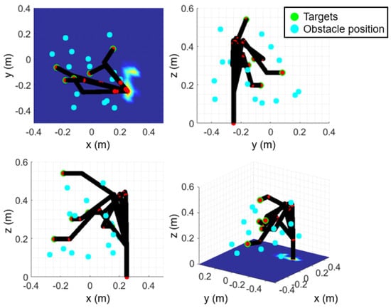
Figure 6.
All the postures of the manipulator at the selected position with the selected orientation.

Figure 7.
Inverse Reachability map without assigning negative values: (a–e) for each target and (f) for the aggregate target.
3. Collision-Free Path Planning
3.1. Artificial Potential Field
Artificial potential field (APF) is a path planning method that uses a virtual potential field, inducing attraction towards the destination and repulsion near obstacles. Compared to other path planning methods, APF is widely used due to its simplicity and low computational requirements. The repulsive potential field for obstacle i, , was constructed based on a quadratic form [32]:
where represents the position of joint, represents the position of obstacle i, is the euclidean distance between and , is the safety distance for obstacle i, and is the repulsive gain.
3.2. Model Predictive Artificial Potential Field
This paper introduces model predictive artificial potential field (MPAPF), a method that formulates a nonlinear optimization problem to plan paths in joint space using APF. This MPAPF path planning method has the advantage of avoiding the problem of generated paths exiting the manipulator workspace or not accurately considering joint limits. Additionally, collision checks are performed for joint positions as well, ensuring that all points of the manipulator do not collide with the obstacle. Using the APF values of states for multiple steps reduces the risk of local minima compared to APF methods. In the case of APF, the path may get stuck in a local minimum if there is no nearby position with a lower potential value than the current one. However, MPAPF finds a path by minimizing the cumulative potential value over multiple steps, allowing it to move to a higher-potential position if that helps it to escape from a local minimum.
The states at any discrete time instant within the prediction horizon n with sampling time and the angular velocity at time instant k, , are expressed as follows:
Equation (3) can be simply expressed as follows:
where
where m is the number of joints, is the joint angle at time instant k and is an identity matrix.
If are known, the positions of the joints, , can be determined by the forward kinematics. A nonlinear minimization problem can be formulated as follows using the joint positions and angles, along with the positions of the obstacles:
where
where and are constants representing the gains of each function, f is the obstacle avoidance function, g is the target attraction function, and o is the number of obstacles. denotes joint angles when reaching the target from the selected position. Function f uses a repulsive potential function, Equation (2), to avoid obstacles and g acts as an attractive potential to move all joints to the target angle.
In the manipulator used in this paper, each joint has different limits. To ensure that all the joints stay within lower and upper limits during the path planning process, , the following constraints were added to the optimization problem:
The nonlinear optimization problem formulated in Equation (6) was implemented in Python 3.7.6 using the SciPy 1.4.1 optimization library [33].
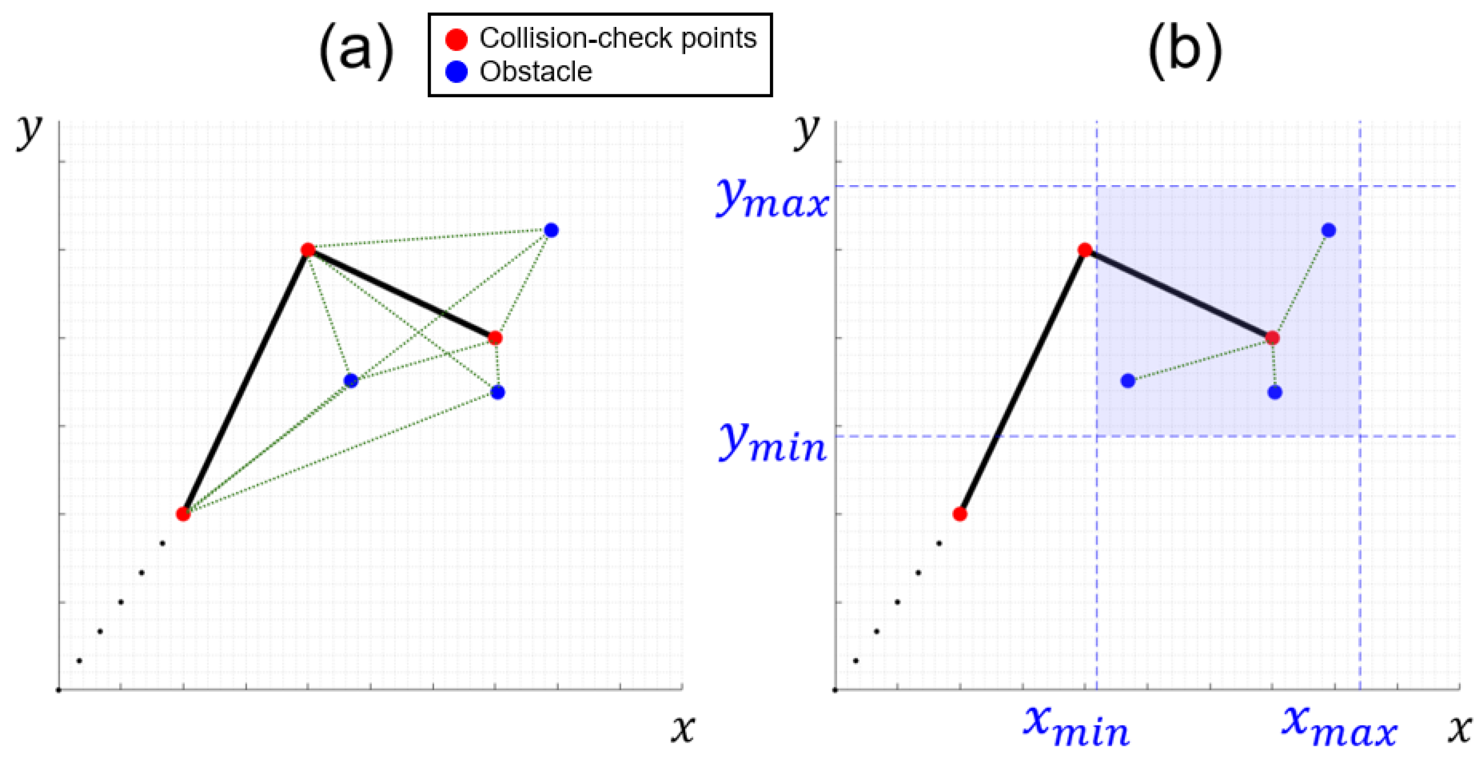
The computational time increases significantly as the number of obstacles increases due to collision checking for all joints and the nonlinearity of the objective function. To mitigate this, feasible groups of obstacles are represented as clusters. For example, in the case of a collision check problem with joints and obstacles, shown in Figure 8, collision checks are conducted between the joints of the manipulator, which are represented by red circles while the obstacles are represented by blue circles. In a problem with three joints and obstacles, Figure 8a requires nine collision checks between all the joints and obstacles. In contrast, it is sufficient to perform three collision checks only between the end-effector and the obstacles located within the clustered range, as shown in Figure 8b. The range of clusters is defined so that the repulsive potential is generated only when a joint is within this range, thereby reducing the amount of computations and thus minimizing the computational time. In this paper, the cluster range is defined by extending the minimum and maximum obstacle coordinates along each axis by the safety distance used in the repulsive potential. The path planning method using MPAPF was validated through simulation in Section 4 and experiments in Section 5.
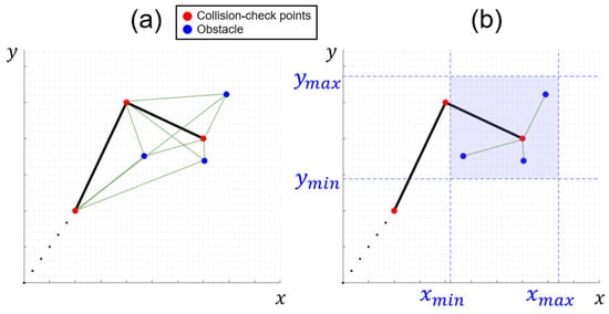
Figure 8.
Example of collision check: (a) point cloud; (b) clustered.
3.3. Comparison to Other Algorithms
Common algorithms used in path planning for robotic manipulators include APF, RRT* and A*. The APF algorithm offers simplicity and fast computation for reaching a goal point but struggles with the inherent issue of local minima. The RRT* algorithm is flexible and adaptable to various environments by randomly expanding a tree, but it can produce inefficient paths and increase computation time due to detours. The A* algorithm guarantees an optimal path but has computational complexity, with excessive grids when dimensionality increases or grid size decreases.
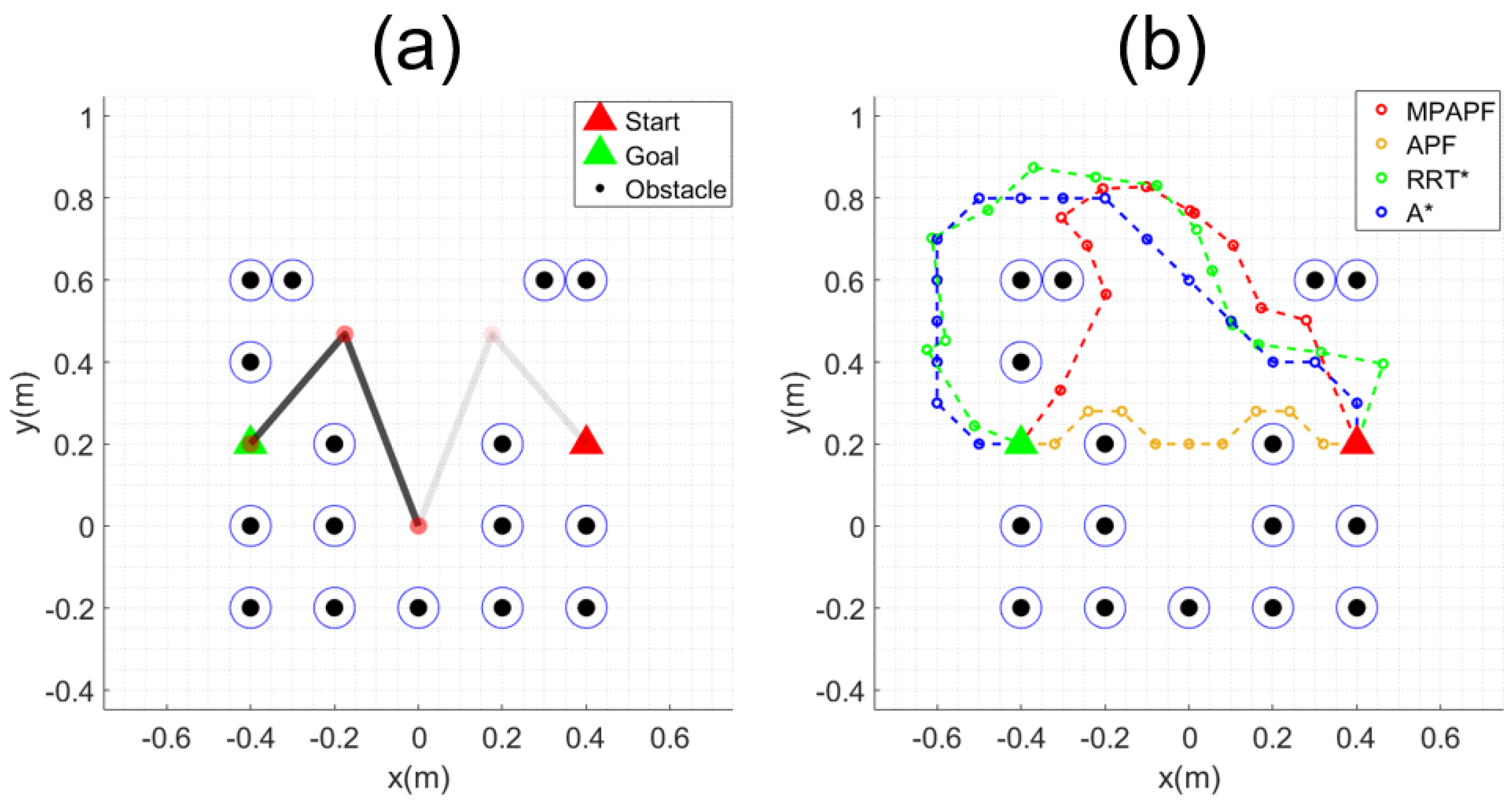
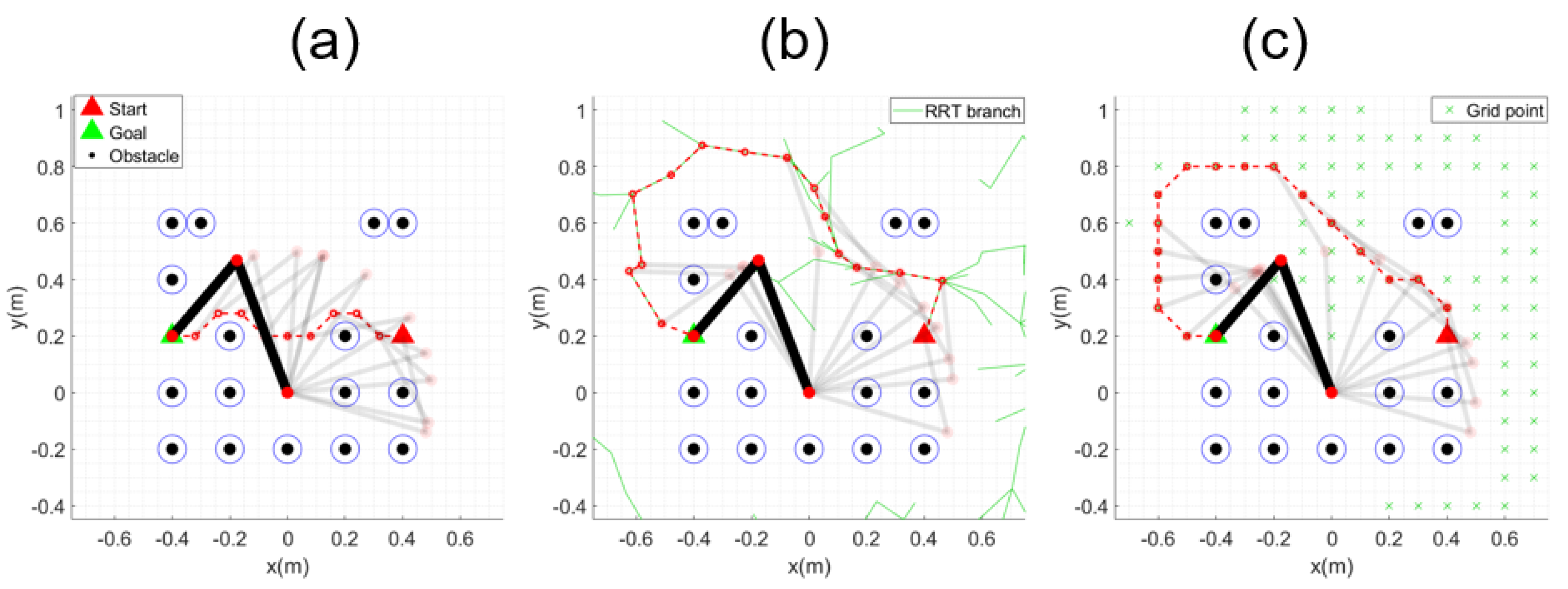
Examples of path planning using the MPAF, APF, RRT* and A* algorithms are illustrated in Figure 9b, where a 2-link manipulator moves from the starting point, represented by a red triangle, to the goal point, represented by a green triangle, in an environment with obstacles represented by black circles, as shown in Figure 9a.
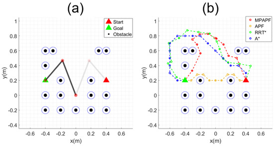
Figure 9.
Example of 2−link manipulator: (a) start and goal configuration; (b) generated path.
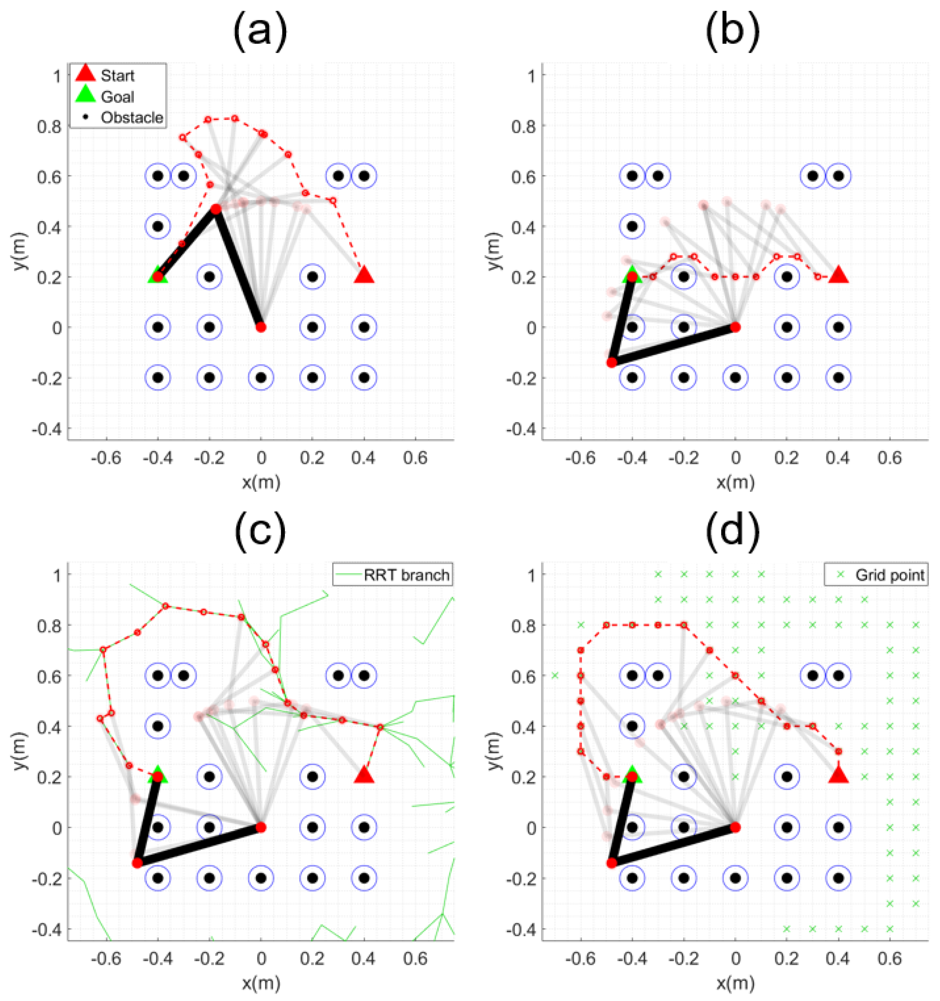
The movement trajectory of the manipulator for all the paths obtained in Figure 9b is shown in Figure 10. All algorithms except MPAPF either fail to find a solution due to exceeding the workspace or lead to collisions, as it is impossible to change from the initial elbow-up configuration to the goal elbow-down configuration. Collisions occur even when using the elbow-down configuration as the initial pose, as shown in Figure 11. Table 1 presents the results corresponding to Figure 10 and Figure 11. The safety distance was set to 0.05 m, and the table shows the minimum distances between each link center and the surrounding obstacles. Collisions occurred in all algorithms except MPAPF. In particular, when using RRT* and A*, the generated paths extend beyond the manipulator’s workspace, indicating that these methods are invalid for this task.
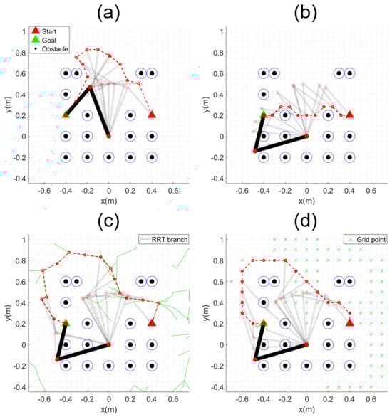
Figure 10.
Example of path planning: (a) MPAPF; (b) APF; (c) RRT*; (d) A*. The dotted red lines are the generated paths, and the transparent traces represent intermediate steps.
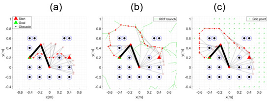
Figure 11.
Example of multiple solution: (a) APF; (b) RRT*; (c) A*. The dotted red lines are the generated paths, and the transparent traces represent intermediate steps.

Table 1.
Minimum distance and validity check for each algorithm.
The generated paths must be converted to joint-space paths through post-processing. The velocity trajectory and the inverse Jacobian matrix are generally used to convert paths to joint space, since multiple solutions may exist when solving inverse kinematics directly for the generated path points. Even in this approach, the Jacobian matrix may not have an inverse depending on configuration of the manipulator leading to constraints in posture adjustment [34]. The Jacobian matrix may not be a square matrix when redundancies exist in the manipulator, making it difficult to achieve accurate conversion. Further, all of these algorithms, except for MPAPF, are point-based path planning methods and therefore cannot consider the geometry of the manipulator. Only the end-effector is considered fundamentally, leaving collisions at other points on the manipulator, joint limits, and the manipulator workspace entirely unaccounted for.
In contrast to point-based path planning algorithms, MPAPF allows the geometry of the manipulator to be considered through forward kinematics, enabling collision checking at all points on the manipulator and posture changes. A smooth path is generated without post-processing, as shown in Figure 10a, and since inverse kinematics is not used during path planning, the problem of multiple solutions does not need to be addressed.
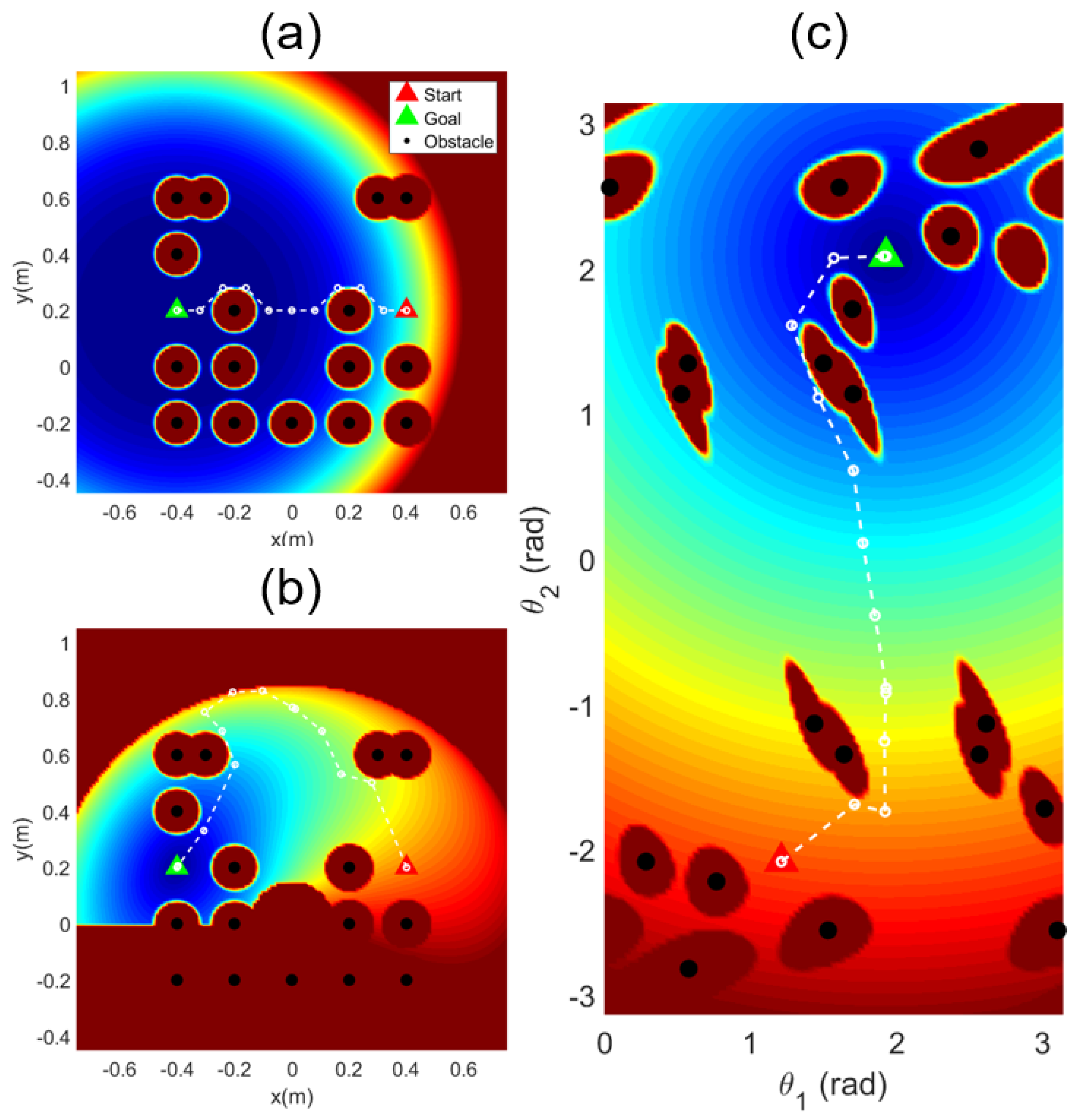
The example potential maps using simple APF and MPAPF are shown in Figure 12. Red and blue respectively represent the maximum and minimum values of the potential field, with yellow in the middle. Virtual obstacles [35] or forces [36] to modify the potential map near local minima were proposed to address the local minimum problem. However, these methods can only help in local areas and a repetitive problem may occur where the object could return to the same spot. The potential map with MPAPF is formed in the joint space. The structure of the potential map with MPAPF is complicatedly transformed, as shown in Figure 12c, which helps reduce the probability of local minima. The paths are computed to minimize the sum of potential values over several discrete-time steps, allowing for movement toward areas with higher potential values if needed. This characteristic further reduces the risk of being trapped in local minima. Since the potential map expands depending on the number of joints, the complexity of the map increases as the number of joints increases. Figure 12b is for visualization purposes to illustrate the potential map in the -space workspace, so it may differ from the actual potential map.
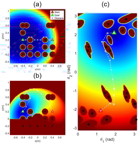
Figure 12.
Example of potential map: (a) APF; (b) MPAPF in xy-space; (c) MPAPF in joint space.
4. Simulation
4.1. Simulation Setup
To validate the proposed methods, we constructed a simulator modeling a Kanpei orchard similar to real-world conditions. The simulator was built using GAZEBO and ROS kinetic on Ubuntu 16.04, running on a system with a 64-bit Intel(R) Core(TM) i7-7700K CPU running at 4.20 GHz. All The algorithms were implemented in Python.
The mobile manipulator consisted of Robotis’ RH-P12 gripper mounted on an Open-Manipulator pro, which was placed on Clearpath Robotics’ Ridgeback UGV equipped with Omni-directional wheels, as shown in Figure 13. The Kanpei trees were strategically placed inside obstacles formed by other trees to complicate the approach for the mobile manipulator. The fruits were modeled to resemble their real counterparts, with a diameter of approximately 10 cm. The modeling of Kanpei trees and the orchard is illustrated in Figure 14.
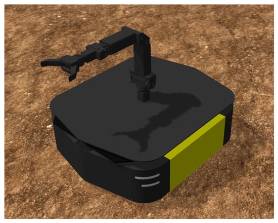
Figure 13.
Mobile manipulator;Ridgeback UGV with Open−Manipulator pro and RH−P12 gripper.
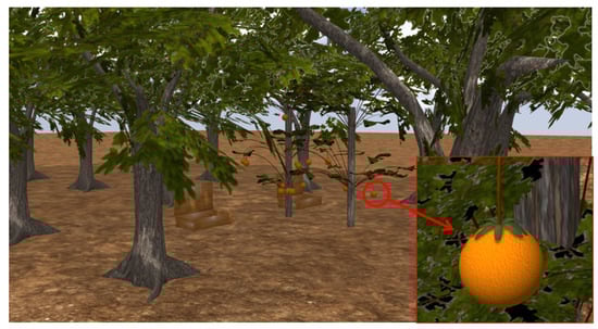
Figure 14.
Simulator model of orchard and kanpei.
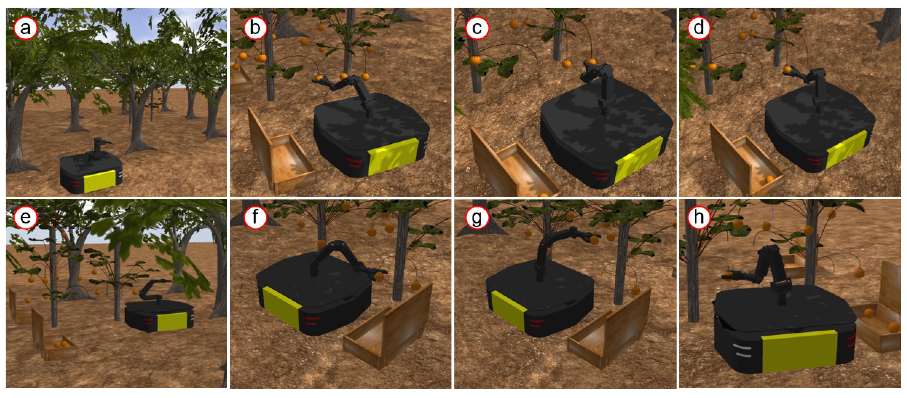
It was assumed that the positions of all the trees and fruits were known through orchard mapping via a vision system. The harvesting scenario has two parts: First, the closest three fruits to the initial position of the robot were selected for harvesting. Fixed positions of UGV and the orientation for approaching a target fruit of the end-effector for the target fruits were selected using IRM. Then, the UGV path to the selected position and harvesting paths of the manipulator for each fruit from that position were generated using MPAPF and executed. Second, the same procedure was repeated for harvesting three fruits placed behind trees. Harvesting paths of the manipulator were generated only from initial basket placement to fruits and repeated to return to the initial in reverse.
4.2. Simulation Result
The simulation results using the implemented simulator and algorithms are illustrated in Figure 15. The first part is shown in Figure 15a–d, and the second part in Figure 15e–h. The mobile base moves to the selected position, as shown in Figure 15a, and then the manipulator harvests the target fruits, as shown in Figure 15b–d. The same procedure was repeated for other targets, as shown in Figure 15e–h. The generated paths for the UGV are shown in Figure 16. In each simulation part, the initial positions are represented in red, the selected final positions from IRM in green, and the mapped obstacle trees in brown circles. The intermediate paths from the initial position to the selected final position were generated by MPAPF and are represented in blue. The computation times for position and orientation selections were 2.064 and 1.831 s for the first and second parts, respectively. The path planning computation times were 0.114 and 0.04 s for the first and second parts, respectively. Ten and six path points were generated, and the paths were set up for the mobile base to pass through the points sequentially without generating trajectories.
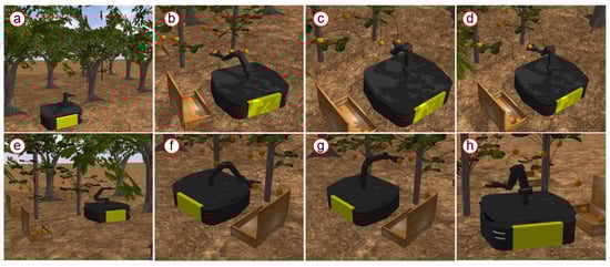
Figure 15.
The progress of the harvest process simulation: (a) approach from initial position to selected location; (b–d) harvesting fruits; (e) approach to another selected location; (f–h) harvesting fruits.
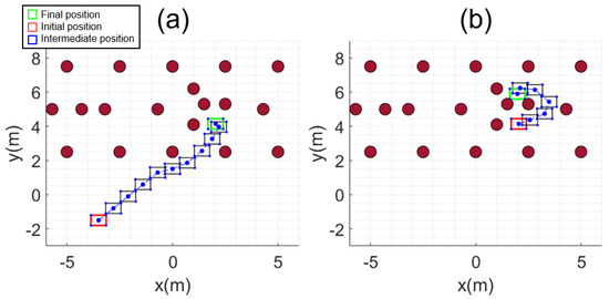
Figure 16.
Path of mobile base: (a) first part; (b) second part.
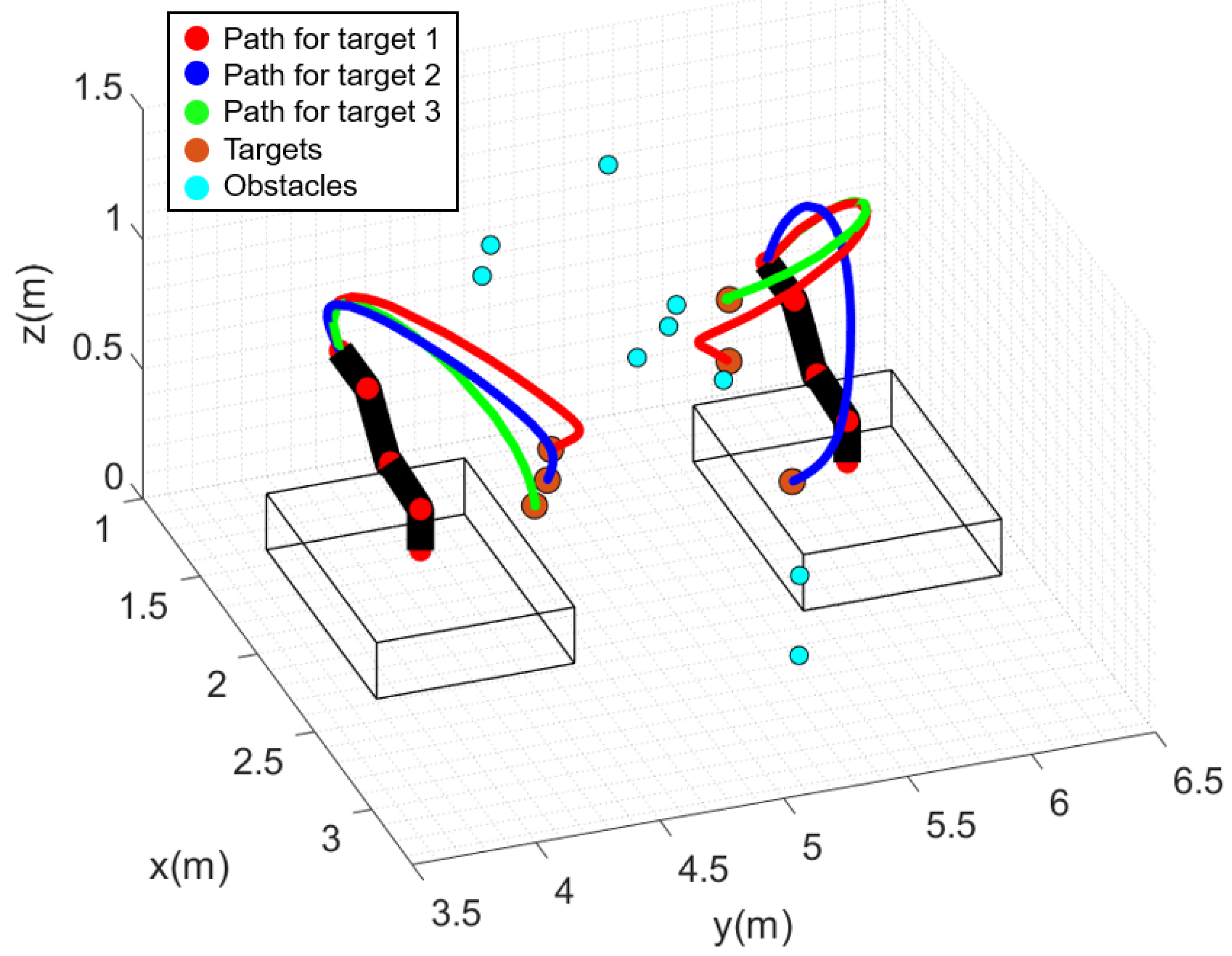
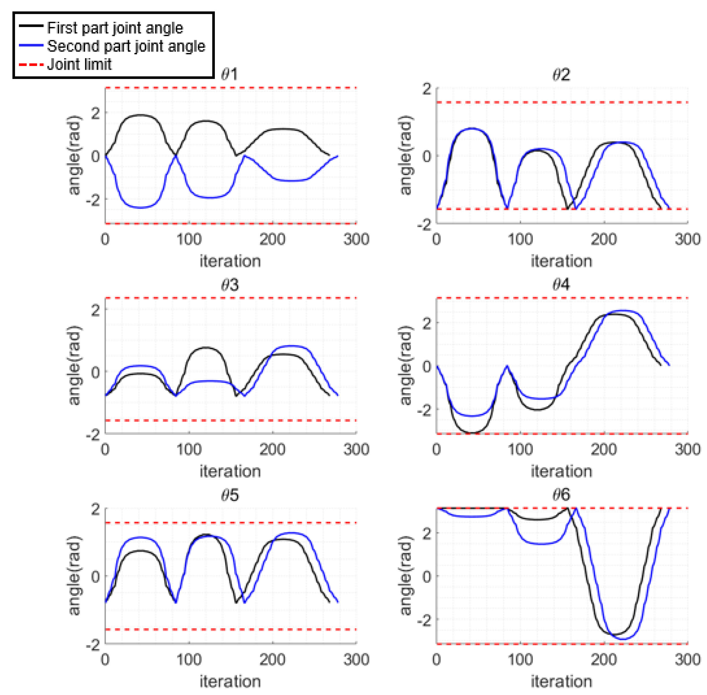
The harvesting paths of the manipulator for each part of harvesting are shown in Figure 17. The paths for harvesting three fruits in each part are shown in red, green, and blue, respectively. The target fruits are represented by the orange circles, while other obstacle fruits are represented by cyan circles. Each generated path ensures collision-free reaching of the target fruits without movement of the base. The computation times for the paths were 2.985, 2.623, 3.923, 2.815, 2.847 and 4.054 s, and the number of path points generated were 84, 74, 110, 84, 82 and 112 for the path planning of each of the six target fruits. The joint angles of the manipulator are shown in Figure 18, where the black and blue solid lines represent the joint angles for the first and second part, respectively, and the red dashed line indicates the joint limits. All the paths were generated to ensure that the joint angles did not exceed their limits.
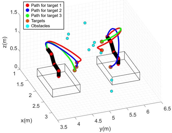
Figure 17.
Harvesting paths of the manipulator for each simulation part.

Figure 18.
Joint angles of manipulator at each part of harvesting.
5. Experiment
5.1. Experiment Setup
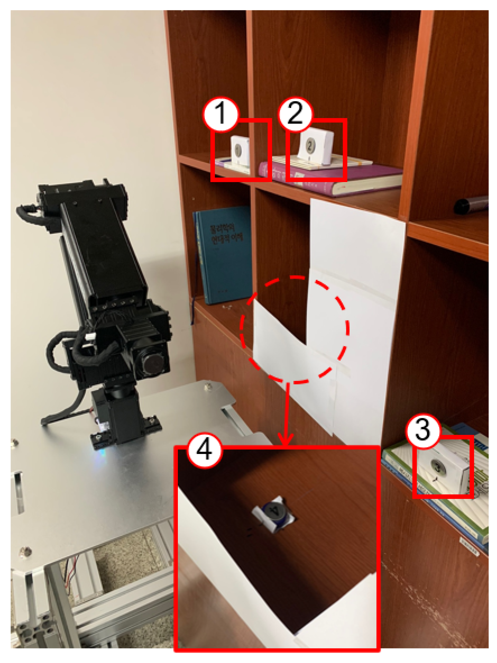
To validate the collision-free path planning using the proposed MPAPF, experiments were conducted in a complex situation only for collision-free path planning. The manipulator was fixed at an arbitrary position without a mobile base due to the limitations of the experimental environment. As shown in Figure 19, the experiment environment consisted of a shelf with four targets, one of which was placed behind a partition to make it difficult to approach.

Figure 19.
Experiment environment. Four targets are shown inside the red boxes and the circled numbers indicate their picking sequence.
The experiments were conducted under the assumption that the positions of obstacles and targets were known without sensors for detecting the environment. Both the shelf and the partition were represented in the form of point clouds. As mentioned in Section 3, in order to reduce computation time, all shelf parts and partition were represented as clusters. The distance threshold between obstacle clusters and joints was set to 100 mm and the safety distance for the repulsive potential was set to 50 mm. All point clouds were structured at intervals of 50 mm and 110 points for the shelf and 44 points for the partitions, respectively. The position selection algorithm was not applied and only the experiment verification of collision-free path planning was conducted. The target object arrival orientations were arbitrarily set. The paths from the initial posture to each target were generated using MPAPF and were organized to return to the initial position in reverse. The same manipulator and system were used in the experiment as in the simulator. The experiment was conducted by directly inputting the joint trajectory calculated on the PC into the manipulator through U2D2 communication converter by Robotis. The manipulator was equipped with an integrated device—DYNAMIXEL by Robotis—which allows the user to input an angle value, enabling the robot to follow it without requiring a controller or driver. The overall environment system diagram is shown in Figure 20.
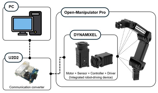
Figure 20.
System diagram.
5.2. Experiment Result
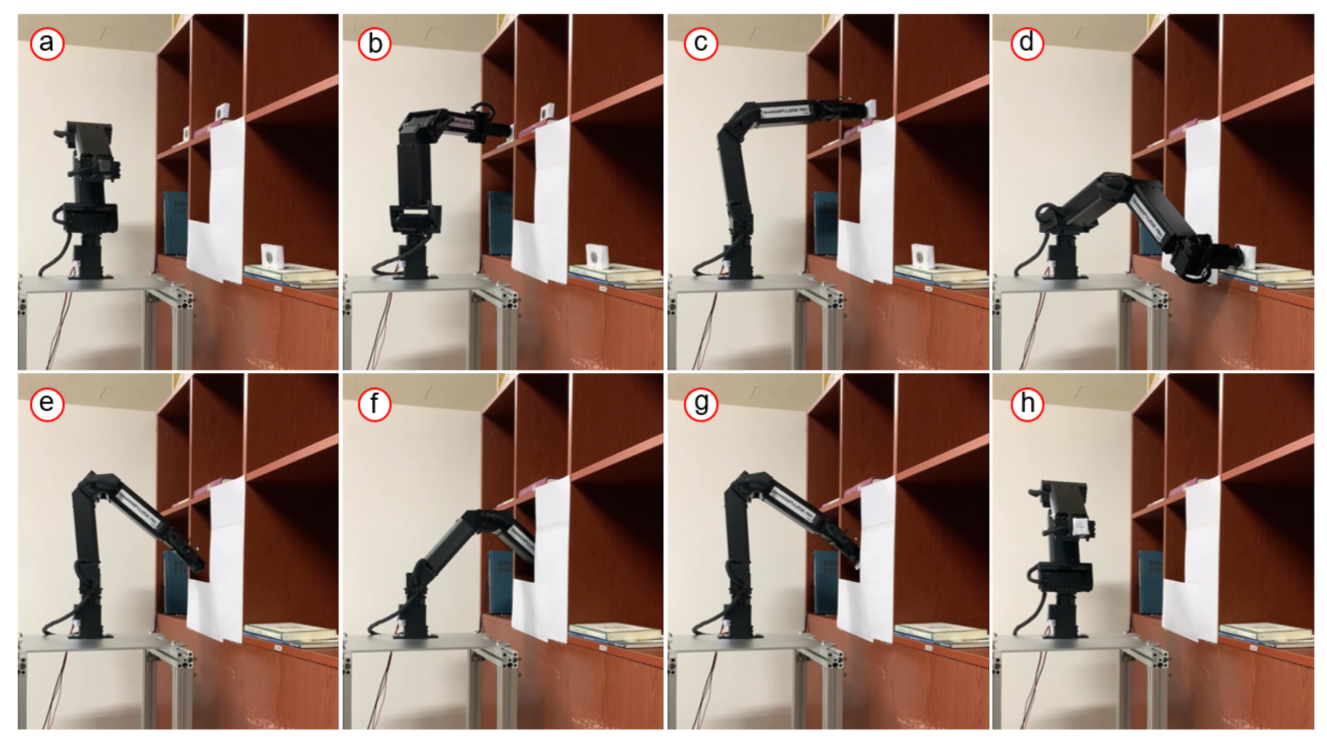
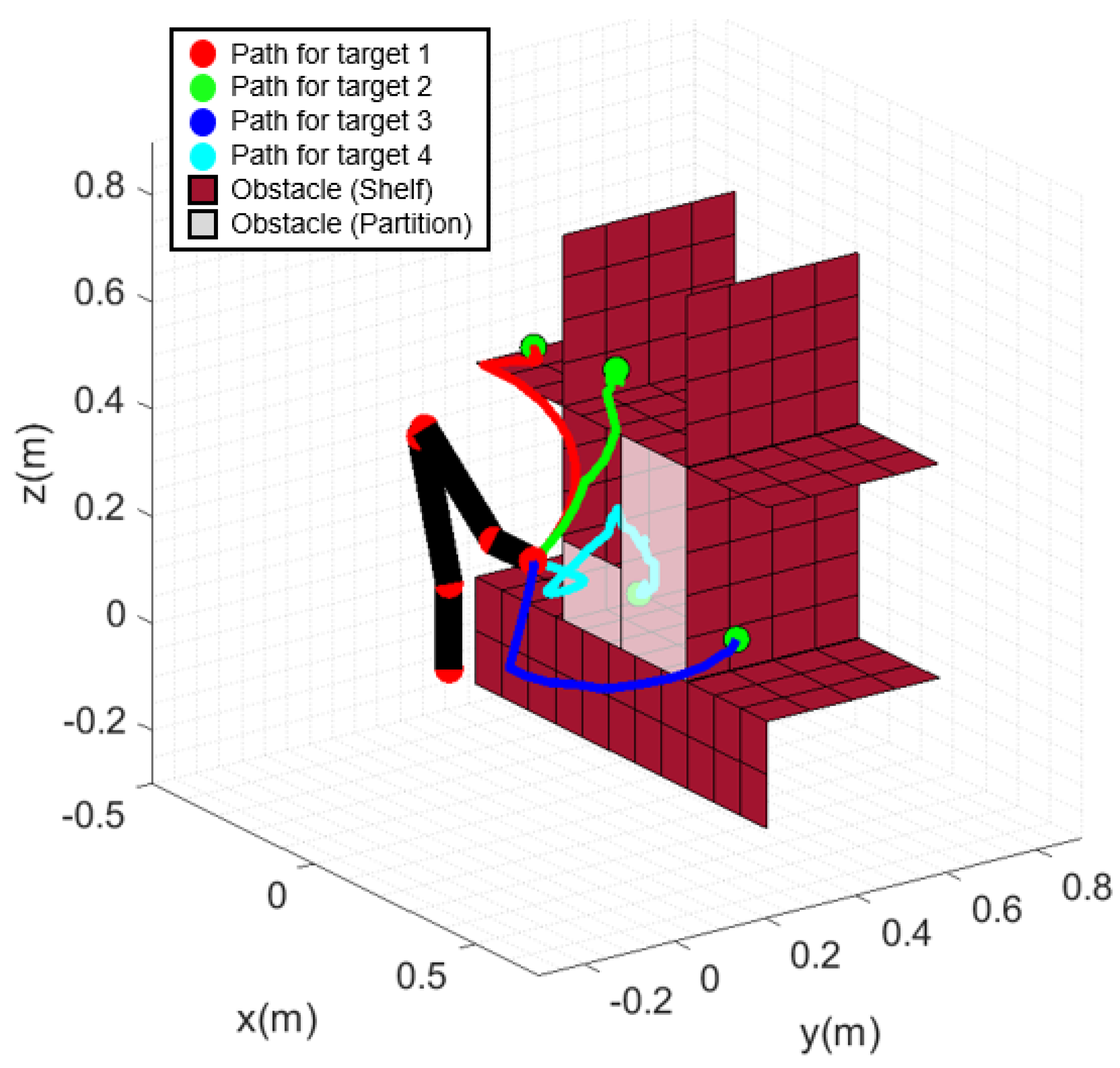
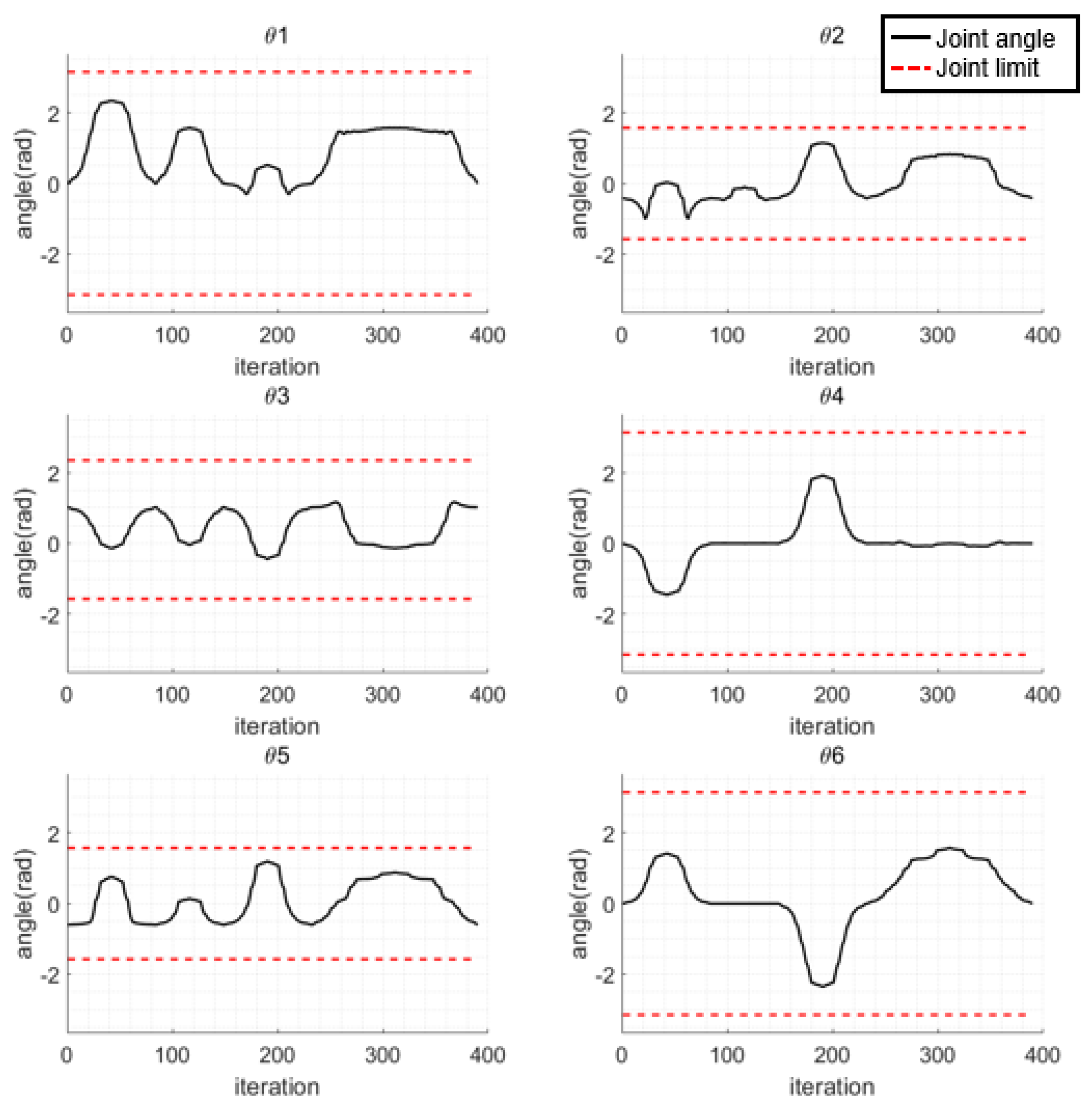
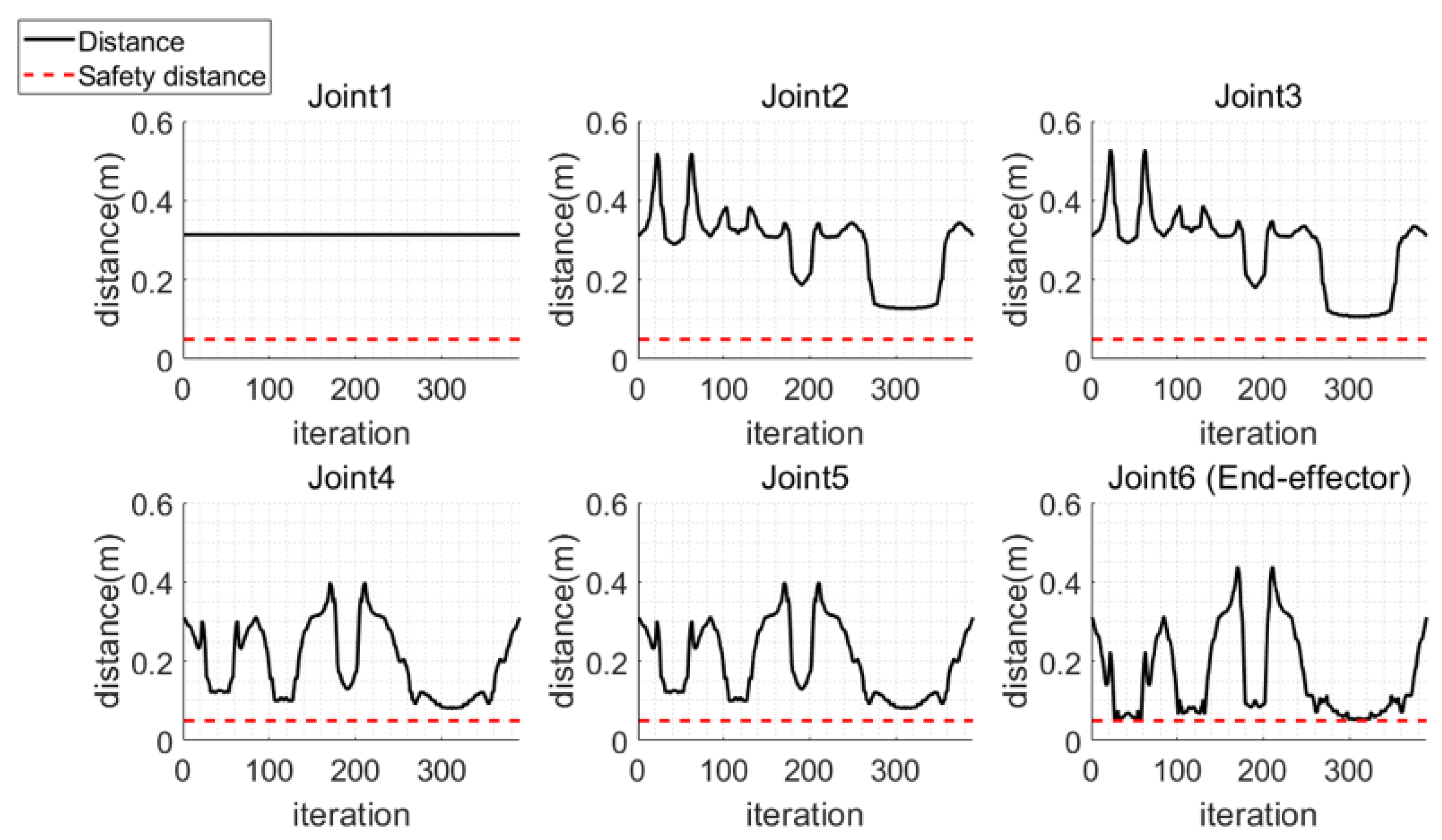
The experiment results of applying collision-free path planning using MPAPF to the manipulator are shown in Figure 21. In Figure 21a, the initial posture is depicted, and in b–d, the manipulator reaches the relatively easily accessible target objects without colliding with the shelf. In e–h, the manipulator approaches the target located behind the partition without colliding with the shelf or the partition. The path computation times were 4.9, 3.8, 4.8 and 45.2 s, respectively. Since the final target is located within the shelf and partition, the manipulator frequently remained closer than the threshold. The computation time was prolonged when approaching the final target due to the dense configuration of the point cloud. Each path consists of 42, 32, 42 and 78 path points. In experiment, the manipulator was operated with a 0.25 s interval between generated path points. The generated paths are shown in Figure 22. The paths to each target object are indicated in red, green, blue and cyan, respectively. As shown in Figure 22, none of the paths overlap with the shelf or partition. Joint angles are shown in Figure 23, where all the generated joint angles are within the joint limit range. The clearances in Figure 24 represent the distances between the positions of all the joints and the obstacles during manipulation, confirming that all parts of the manipulator did not approach closer than the set safety distance.

Figure 21.
The progress of the experiment: (a) initial pose; (b–g) approaching each target; (h) final pose.

Figure 22.
Collision−free paths for each target.
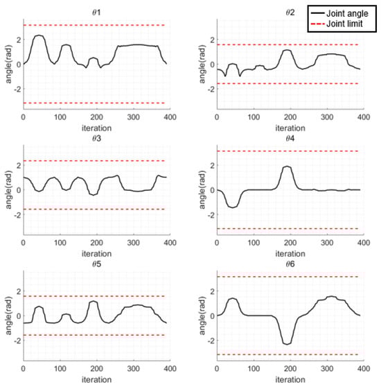
Figure 23.
Joint angles of the manipulator.
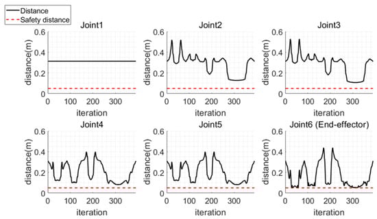
Figure 24.
Clearances between joints and obstacles.
6. Conclusions
In this paper, research on the automation of Kanpei harvesting robots has been conducted. Using the proposed inverse reachability map based algorithm for selecting fruit harvesting positions, it is possible to pre-select advantageous robot system positions for harvesting. This allows for multiple target fruits to be harvested from one fixed location without the overall movement of the robot system, resulting in time and energy savings. Although the fruits to be harvested still need to be determined by humans, it is advantageous to know in advance whether it is possible to harvest using only the manipulator without moving the base. And MPAPF was proposed for collision-free path planning that not only considers the end-effector but also the manipulator as a whole. Since the path is planned in joint space, the end-effector does not exceed the workspace, and the joint limits are also considered. By adding the target angle to the objective function and calculating the potential for multiple points, the problem of falling into local minima, which is a persistent issue encountered with APF, can be mitigated to some extent. Through simulations, successful harvesting of multiple fruits is possible using the position selection and path planning algorithms. Furthermore, experiments showed that collision-free paths are well-planned even in complex environments. However, the computation time increases significantly as the number of obstacles increases; therefore, improvements in the algorithm will be further pursued. Moreover, the entire system, including the mobile base, a vision system, and new types of end-effector, will be developed for experimental validation in a real Kanpei harvesting environment.
Author Contributions
Conceptualization, Y.C.; methodology, Y.C.; software, Y.C.; validation, Y.C.; formal analysis, Y.C.; investigation, Y.C.; resources, Y.C.; data curation, D.C.; writing—original draft preparation, Y.C.; writing—review and editing, J.H.P.; visualization, Y.C.; supervision, J.H.P.; project administration, K.K.; funding acquisition, D.C. All authors have read and agreed to the published version of the manuscript.
Funding
This research was supported by the Ministry of Trade, Industry and Energy (MOTIE) and the Korea Evaluation Institute of Industrial Technology (KEIT) under Grant RS-2024-00443400 and by the Korea Institute of Planning and Evaluation for Technology in Food, Agriculture, and Forestry (IPET) through the Open Field Smart Agriculture Technology Short-term Advancement Program, funded by the Ministry of Agriculture, Food and Rural Affairs (MAFRA) under Grant 122032-03-2-HD020.
Institutional Review Board Statement
Not applicable.
Informed Consent Statement
Not applicable.
Data Availability Statement
Data are contained within the article.
Conflicts of Interest
The authors declare no conflicts of interest.
References
- Mahmud, M.S.A.; Abidin, M.S.Z.; Emmanuel, A.A.; Hasan, H.S. Robotics and automation in agriculture: Present and future applications. Appl. Model. Simul. 2020, 4, 130–140. [Google Scholar]
- Bogue, R. Fruit picking robots: Has their time come? Emerald Insight Ind. Robot. 2020, 47, 141–145. [Google Scholar] [CrossRef]
- Mohamed, E.S.; Belal, A.A.; Abd-Elmabod, S.K.; El-Shirbeny, M.A.; Gad, A.; Zahran, M.B. Smart farming for improving agricultural management. Egypt. J. Remote Sens. Space Sci. 2021, 24, 971–981. [Google Scholar] [CrossRef]
- Onishi, Y.; Yoshida, T.; Kurita, H.; Fukao, T.; Arihara, H.; Iwai, A. An automated fruit harvesting robot by using deep learning. ROBOMECH J. 2019, 6, 1–8. [Google Scholar] [CrossRef]
- Nguyen, T.T.; Vandevoorde, K.; Wouters, N.; Kayacan, E.; De Baerdemaeker, J.G.; Saeys, W. Detection of red and bicoloured apples on tree with an RGB-D camera. Biosyst. Eng. 2016, 146, 33–44. [Google Scholar] [CrossRef]
- Yoshida, T.; Kawahara, T.; Fukao, T. Fruit recognition method for a harvesting robot with RGB-D cameras. ROBOMECH J. 2022, 9, 15. [Google Scholar] [CrossRef]
- Lin, G.; Tang, Y.; Zou, X.; Xiong, J.; Fang, Y. Color-, depth-, and shape-based 3D fruit detection. Precis. Agric. 2020, 21, 1–17. [Google Scholar] [CrossRef]
- Lin, G.; Tang, Y.; Zou, X.; Li, J.; Xiong, J. In-field citrus detection and localisation based on RGB-D image analysis. Biosyst. Eng. 2019, 186, 34–44. [Google Scholar] [CrossRef]
- Lin, G.; Tang, Y.; Zou, X.; Xiong, J.; Li, J. Guava detection and pose estimation using a low-cost RGB-D sensor in the field. Sensors 2019, 19, 428. [Google Scholar] [CrossRef]
- Zhou, H.; Wang, X.; Au, W.; Kang, H.; Chen, C. Intelligent robots for fruit harvesting: Recent developments and future challenges. Precis. Agric. 2022, 23, 1856–1907. [Google Scholar] [CrossRef]
- Hadas, E.; Jozkow, G.; Walicka, A.; Borkowski, A. Apple orchard inventory with a LiDAR equipped unmanned aerial system. Int. J. Appl. Earth Observ. Geoinf. 2019, 82, 101911. [Google Scholar] [CrossRef]
- Tsoulias, N.; Paraforos, D.S.; Xanthopoulos, G.; Zude-Sasse, M. Apple shape detection based on geometric and radiometric features using a LiDAR laser scanner. Remote Sens. 2020, 2481. [Google Scholar] [CrossRef]
- Gené-Mola, J.; Gregorio, E.; Guevara, J.; Auat, F.; Sanz-Cortiella, R.; Escolà, A.; Llorens, J.; Morros, J.R.; Ruiz-Hidalgo, J.; Vilaplana, V.; et al. Fruit detection in an apple orchard using a mobile terrestrial Laser Scanner. Biosyst. Eng. 2019, 18, 171–184. [Google Scholar] [CrossRef]
- Underwood, J.P.; Jagbrant, G.; Nieto, J.I.; Sukkarieh, S. Lidar-based tree recognition and platform localization in orchards. J. Field Robot. 2015, 32, 1056–1074. [Google Scholar] [CrossRef]
- Gao, P.; Jiang, J.; Song, J.; Xie, F.; Bai, Y.; Fu, Y.; Wang, Z.; Zheng, X.; Xie, S.; Li, B. Canopy volume measurement of fruit trees using robotic platform loaded LiDAR data. IEEE Access 2021, 9, 156246–156259. [Google Scholar] [CrossRef]
- Rivera, G.; Porras, R.; Florencia, R.; Sánchez-Solís, J.P. LiDAR applications in precision agriculture for cultivating crops: A review of recent advances. Comput. Electron. Agric. 2023, 207, 107737. [Google Scholar] [CrossRef]
- Tagarakis, A.C.; Filippou, E.; Kalaitzidis, D.; Benos, L.; Busato, P.; Bochtis, D. Proposing UGV and UAV systems for 3D mapping of orchard environments. Sensors 2022, 22, 1571. [Google Scholar] [CrossRef]
- Van Henten, E.J.; Hemming, J.; Van Tuijl, B.A.J.; Kornet, J.G.; Bontsema, J. Collision-free motion planning for a cucumber picking robot. Biosyst. Eng. 2003, 86, 135–144. [Google Scholar] [CrossRef]
- Ye, L.; Duan, J.; Yang, Z.; Zou, X.; Chen, M.; Zhang, S. Collision-free motion planning for the litchi-picking robot. Comput. Electron. Agric. 2021, 185, 106151. [Google Scholar] [CrossRef]
- Kuffner, J.; LaValle, S.M. RRT-Connect: An efficient approach to single-query path planning. In Proceedings of the IEEE International Conference on Robotics and Automation, San Francisco, CA, USA, 24–28 April 2000. [Google Scholar]
- Cao, X.; Zou, X.; Jia, C.; Chen, M.; Zeng, Z. RRT-based path planning for an intelligent litchi-picking manipulator. Comput. Electron. Agric. 2019, 156, 105–118. [Google Scholar] [CrossRef]
- Liu, C.; Feng, Q.; Tang, Z.; Wang, X.; Geng, J.; Xu, L. Motion planning of the citrus-picking manipulator based on the TO-RRT algorithm. Agriculture 2022, 12, 581. [Google Scholar] [CrossRef]
- Tang, Z.; Xu, L.; Wang, Y.; Kang, Z.; Xie, H. Collision-free motion planning of a six-link manipulator used in a citrus picking robot. Appl. Sci. 2021, 11, 11336. [Google Scholar] [CrossRef]
- Bac, C.W.; Van Henten, E.J.; Hemming, J.; Edan, Y. Harvesting robots for high-value crops: State-of-the-art review and challenges ahead. J. Field Robot. 2014, 31, 888–911. [Google Scholar] [CrossRef]
- Yin, H.; Sun, Q.; Ren, X.; Guo, J.; Yang, Y.; Wei, Y.; Huang, B.; Chai, X.; Zhong, M. Development, integration, and field evaluation of an autonomous citrus-harvesting robot. J. Field Robot. 2023, 40, 1363–1387. [Google Scholar] [CrossRef]
- Wang, D.; Dong, Y.; Lian, J.; Gu, D. Adaptive end-effector pose control for tomato harvesting robots. J. Field Robot. 2023, 40, 535–551. [Google Scholar] [CrossRef]
- Silwal, A.; Davidson, J.R.; Karkee, M.; Mo, C.; Zhang, Q.; Lewis, K. Design, integration, and field evaluation of a robotic apple harvester. J. Field Robot. 2017, 34, 1140–1159. [Google Scholar] [CrossRef]
- Arad, B.; Balendonck, J.; Barth, R.; Ben-Shahar, O.; Edan, Y.; Hellström, T.; Hemming, J.; Kurtser, P.; Ringdahl, O.; Tielen, T.; et al. Development of a sweet pepper harvesting robot. J. Field Robot. 2020, 37, 1027–1039. [Google Scholar] [CrossRef]
- Jun, J.; Kim, J.; Seol, J.; Kim, J.; Son, H.I. Towards an efficient tomato harvesting robot: 3D perception manipulation and end-effector. IEEE Access 2021, 9, 17631–17640. [Google Scholar] [CrossRef]
- Acosta Núñez, J.F.; Andaluz Ortiz, V.H.; González-de-Rivera Peces, G.; Garrido Salas, J. Energy-Saver Mobile Manipulator Based on Numerical Methods. Electronics 2019, 8, 1100. [Google Scholar] [CrossRef]
- Yoshikawa, T. Manipulability of robotic mechanisms. Int. J. Robot. Res. 1985, 4, 3–9. [Google Scholar] [CrossRef]
- Khatib, O. Real-time obstacle avoidance for manipulators and mobile robots. Int. J. Robot. Res. 1986, 5, 90–98. [Google Scholar] [CrossRef]
- Virtanen, P.; Gommers, R.; Oliphant, T.E.; Haberl, M.; Reddy, T.; Cournapeau, D.; Burovski, E.; Peterson, P.; Weckesser, W.; Bright, J.; et al. SciPy 1.0: Fundamental algorithms for scientific computing in Python. Nat. Methods 2020, 17, 261–272. [Google Scholar] [CrossRef] [PubMed]
- Kim, J.; Jie, W.; Kim, H.; Lee, M.C. Modified configuration control with potential field for inverse kinematic solution of redundant manipulator. IEEE/ASME Trans. Mechatron. 2021, 26, 1782–1790. [Google Scholar] [CrossRef]
- Park, M.G.; Lee, M.C. A new technique to escape local minimum in artificial potential field based path planning. KSME Int. J. 2003, 17, 1876–1885. [Google Scholar] [CrossRef]
- Lee, J.; Nam, Y.; Hong, S. Random force based algorithm for local minima escape of potential field method. In Proceedings of the IEEE International Conference on Control Automation Robotics & Vision, Singapore, 7–10 December 2010. [Google Scholar]


Disclaimer/Publisher’s Note: The statements, opinions and data contained in all publications are solely those of the individual author(s) and contributor(s) and not of MDPI and/or the editor(s). MDPI and/or the editor(s) disclaim responsibility for any injury to people or property resulting from any ideas, methods, instructions or products referred to in the content. |
© 2025 by the authors. Licensee MDPI, Basel, Switzerland. This article is an open access article distributed under the terms and conditions of the Creative Commons Attribution (CC BY) license (https://creativecommons.org/licenses/by/4.0/).