
Bearing Fault Diagnosis Method Based on Improved VMD and Parallel Hybrid Neural Network


Abstract
:1. Introduction
- (1)
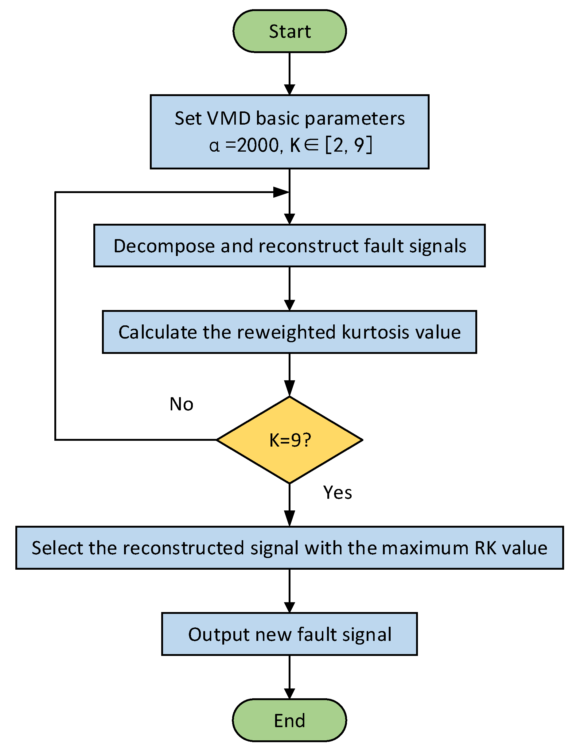
- An improved VMD algorithm is proposed by combining VMD with reweighted kurtosis. Using the reweighted kurtosis value as the evaluation index, the influence of some strong shocks in the fault signal can be eliminated, and the accuracy of fault diagnosis can be improved.
- (2)
- A parallel hybrid neural network model is proposed, which fuses the features extracted by the two parallel networks to achieve feature enhancement and complementarity, which can improve the classification accuracy of the diagnosis model.
- (3)
- The proposed fault diagnosis method is compared with several latest bearing fault diagnosis models. The proposed method has certain advantages in the accuracy of fault diagnosis, which reflects the positives of the method.
2. Model Construction Principle
2.1. Variational Mode Decomposition
2.2. Reweighted Kurtosis Method
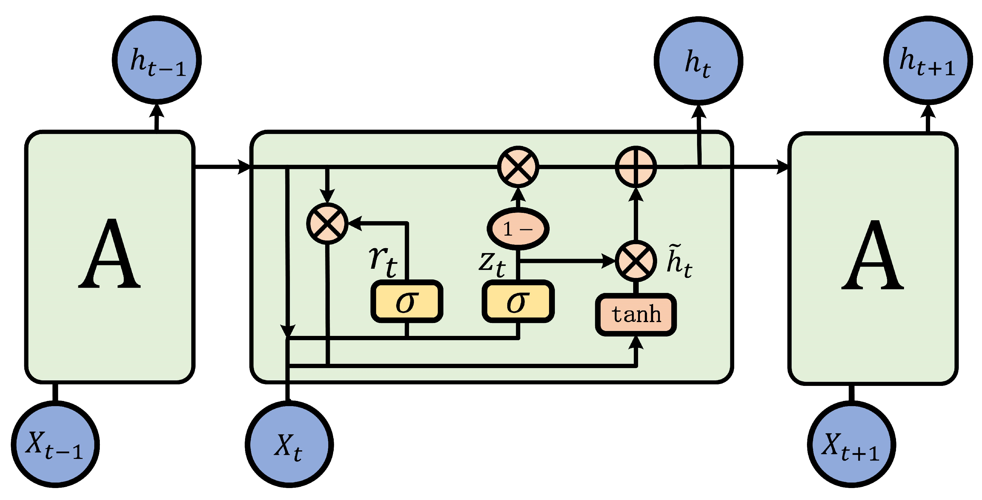
2.3. Recurrent Neural Network
2.4. Convolutional Neural Network
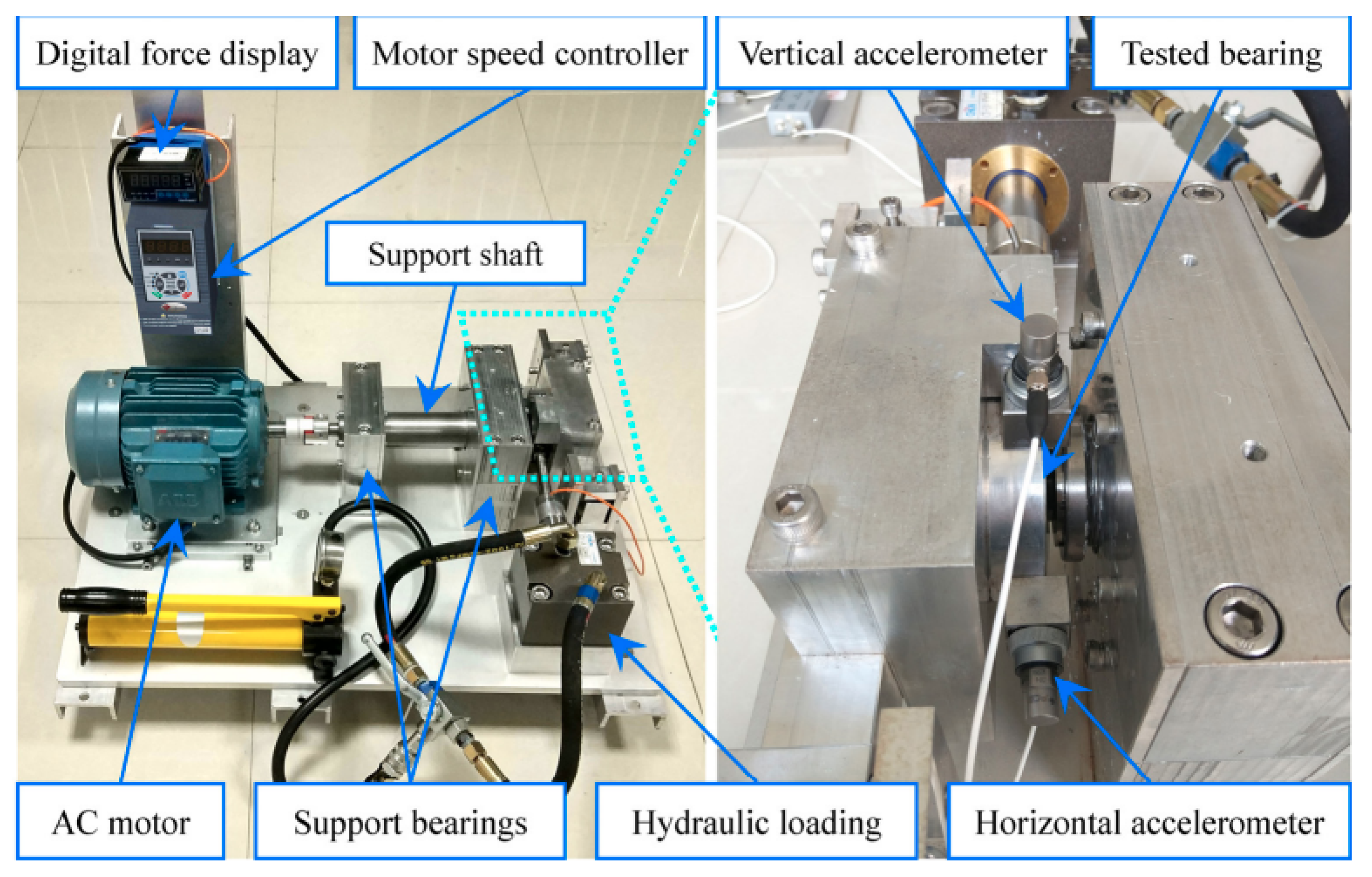
3. Materials and Methods
3.1. Fault Signal Processing Method
3.2. Fault Diagnosis Model Design
3.3. Data Set Processing
4. Results
4.1. Fault Signal Processing
4.2. Fault Diagnosis Model Based on Parallel Hybrid Neural Network
5. Discussion
5.1. Comparison of Denoising Experiments
5.2. Experimental Results and Comparative Analysis
5.3. Generality Analysis
6. Conclusions
Author Contributions
Funding
Institutional Review Board Statement
Informed Consent Statement
Data Availability Statement
Acknowledgments
Conflicts of Interest
Abbreviations
| VMD | Variational mode decomposition |
| RK | Reweighted kurtosis |
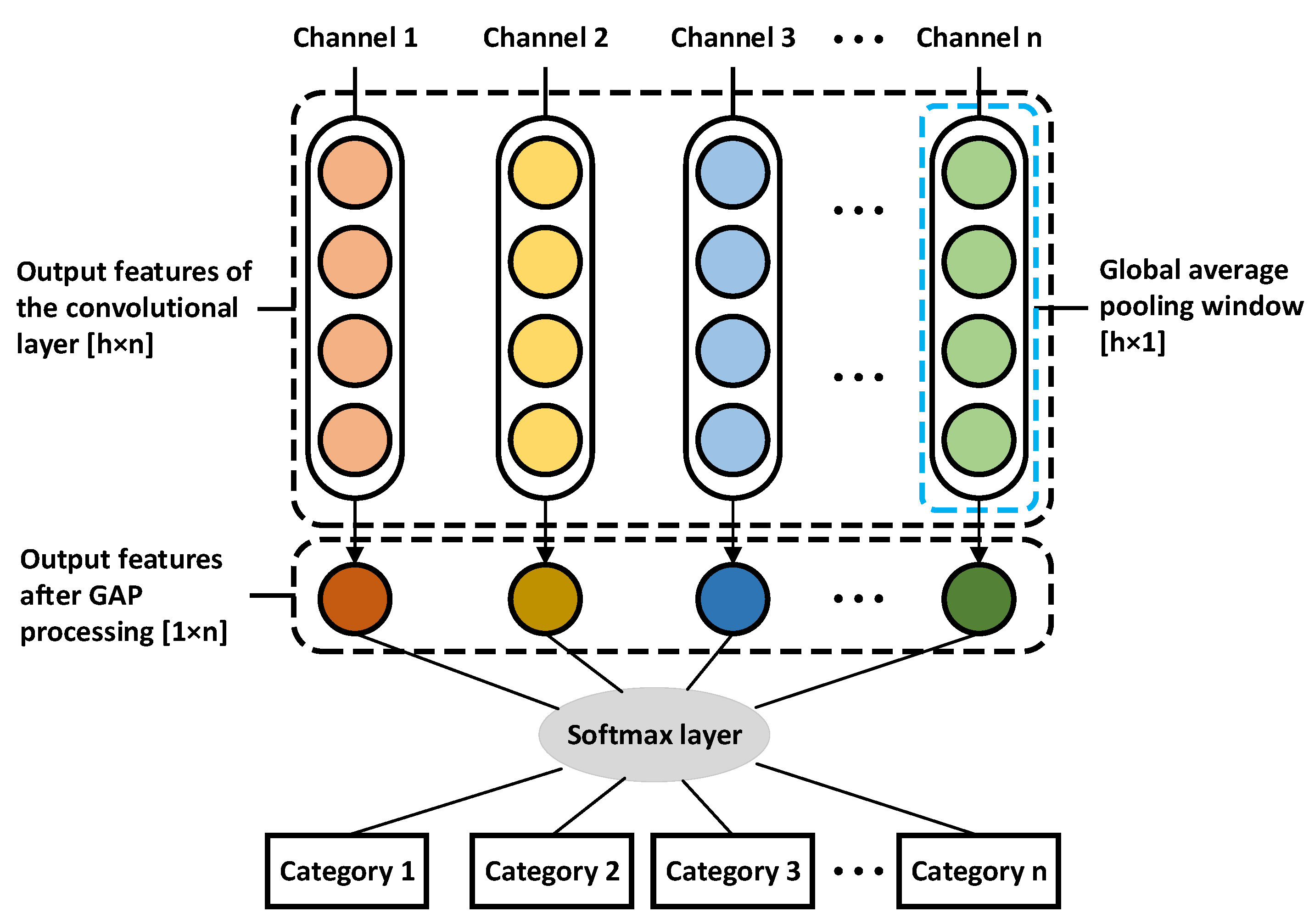
| GAP | Global Average Pooling Layer |
| EMD | Empirical mode decomposition |
| LMD | Local means decomposition |
| IMF | Intrinsic mode functions |
| RNN | Recurrent neural network |
| BiLSTM | Bidirectional long short-term memory |
| BiGRU | Bidirectional gated recurrent unit |
| 1DCNN | One-dimensional Convolutional Neural Network |
| FC | Full connection |
References
- Frosini, L. Novel diagnostic techniques for rotating electrical machines—A review. Energies 2020, 13, 5066. [Google Scholar] [CrossRef]
- Yang, C.; Wang, H.; Gao, Z.; Cui, X. Improving rolling bearing online fault diagnostic performance based on multi-dimensional characteristics. R. Soc. Open Sci. 2018, 5, 180066. [Google Scholar] [CrossRef]
- Ma, Z.; Ruan, W.; Chen, M.; Li, X. An Improved Time-Frequency Analysis Method for Instantaneous Frequency Estimation of Rolling Bearing. Shock Vib. 2018, 2018, 8710190. [Google Scholar] [CrossRef]
- El Khadiri, K.; Elouaham, S.; Nassiri, B.; El Melhaoui, O.; Said, S.; El Kamoun, N.; Zougagh, H. A Comparison of the Denoising Performance Using Capon Time-Frequency and Empirical Wavelet Transform Applied on Biomedical Signal. Int. J. Eng. Appl. 2023, 11, 358–365. [Google Scholar] [CrossRef]
- Meng, D.; Wang, H.; Yang, S.; Lv, Z.; Hu, Z.; Wang, Z. Fault analysis of wind power rolling bearing based on EMD feature extraction. CMES-Comput. Model. Eng. Sci. 2021, 130, 543–558. [Google Scholar] [CrossRef]
- Xu, Y.; Zhang, K.; Ma, C.; Li, S.; Zhang, H. Optimized LMD method and its applications in rolling bearing fault diagnosis. Meas. Sci. Technol. 2019, 30, 125017. [Google Scholar] [CrossRef]
- Torres, M.E.; Colominas, M.A.; Schlotthauer, G.; Flandrin, P. A complete ensemble empirical mode decomposition with adaptive noise. In Proceedings of the 2011 IEEE International Conference on Acoustics, Speech and Signal Processing (ICASSP), Prague, Czech Republic, 22–27 May 2011; pp. 4144–4147. [Google Scholar]
- Colominas, M.A.; Schlotthauer, G.; Torres, M.E. Improved complete ensemble EMD: A suitable tool for biomedical signal processing. Biomed. Signal Process. Control 2014, 14, 19–29. [Google Scholar] [CrossRef]
- Wang, Z.; Wang, J.; Kou, Y.; Zhang, J.; Ning, S.; Zhao, Z. Weak fault diagnosis of wind turbine gearboxes based on MED-LMD. Entropy 2017, 19, 277. [Google Scholar] [CrossRef]
- Liu, Z.; Peng, Y. Study on denoising method of vibration signal induced by tunnel portal blasting based on WOA-VMD algorithm. Appl. Sci. 2023, 13, 3322. [Google Scholar] [CrossRef]
- Li, H.; Wu, X.; Liu, T.; Li, S.; Zhang, B.; Zhou, G.; Huang, T. Composite fault diagnosis for rolling bearing based on parameter-optimized VMD. Measurement 2022, 201, 111637. [Google Scholar] [CrossRef]
- Randall, R.B.; Antoni, J. Rolling element bearing diagnostics—A tutorial. Mech. Syst. Signal Process. 2011, 25, 485–520. [Google Scholar] [CrossRef]
- Sacerdoti, D.; Strozzi, M.; Secchi, C. A comparison of signal analysis techniques for the diagnostics of the IMS rolling element bearing dataset. Appl. Sci. 2023, 13, 5977. [Google Scholar] [CrossRef]
- Shao, S.; Yan, R.; Lu, Y.; Wang, P.; Gao, R.X. DCNN-based multi-signal induction motor fault diagnosis. IEEE Trans. Instrum. Meas. 2019, 69, 2658–2669. [Google Scholar] [CrossRef]
- Zhu, D.; Zhang, Y.; Zhao, L. Fault diagnosis method for rolling element bearing with variable rotating speed using envelope order spectrum and convolutional neural network. J. Intell. Fuzzy Syst. 2019, 37, 3027–3040. [Google Scholar] [CrossRef]
- Shao, Y.; Yuan, X.; Zhang, C.; Song, Y.; Xu, Q. A novel fault diagnosis algorithm for rolling bearings based on one-dimensional convolutional neural network and INPSO-SVM. Appl. Sci. 2020, 10, 4303. [Google Scholar] [CrossRef]
- Chen, H.; Meng, W.; Li, Y.; Xiong, Q. An anti-noise fault diagnosis approach for rolling bearings based on multiscale CNN-LSTM and a deep residual learning model. Meas. Sci. Technol. 2023, 34, 045013. [Google Scholar] [CrossRef]
- Sharma, V.; Parey, A. Extraction of weak fault transients using variational mode decomposition for fault diagnosis of gearbox under varying speed. Eng. Fail. Anal. 2020, 107, 104204. [Google Scholar] [CrossRef]
- Feng, W.; Zhu, Q.; Zhuang, J.; Yu, S. An expert recommendation algorithm based on Pearson correlation coefficient and FP-growth. Clust. Comput. 2019, 22, 7401–7412. [Google Scholar] [CrossRef]
- Pan, H.; Yin, X.; Cheng, J.; Zheng, J.; Tong, J.; Liu, T. Periodic component pursuit-based kurtosis deconvolution and its application in roller bearing compound fault diagnosis. Mech. Mach. Theory 2023, 185, 105337. [Google Scholar] [CrossRef]
- Zhang, X.; Zhang, Z.; Wang, J.; Liu, Z.; Wang, L. Reweighted-Kurtogram with sub-bands rearranged and ensemble dual-tree complex wavelet packet transform for bearing fault diagnosis. Struct. Health Monit. 2022, 21, 2951–2967. [Google Scholar] [CrossRef]
- Chen, L.; Xu, G.; Zhang, S.; Yan, W.; Wu, Q. Health indicator construction of machinery based on end-to-end trainable convolution recurrent neural networks. J. Manuf. Syst. 2020, 54, 1–11. [Google Scholar] [CrossRef]
- Székelyhidi, L. Convolution Type Functional Equations on Topological Abelian Groups; World Scientific: Singapore, 1991; Volume 3. [Google Scholar]
- Zhang, B.; Zhang, S.; Li, W. Bearing performance degradation assessment using long short-term memory recurrent network. Comput. Ind. 2019, 106, 14–29. [Google Scholar] [CrossRef]
- Liu, Z. Bearing Fault Diagnosis of End-to-End Model Design Based on 1DCNN-GRU Network. Discret. Dyn. Nat. Soc. 2022, 2022, 7167821. [Google Scholar]
- Guo, Y.; Mao, J.; Zhao, M. Rolling bearing fault diagnosis method based on attention CNN and BiLSTM network. Neural Process. Lett. 2023, 55, 3377–3410. [Google Scholar] [CrossRef]
- Durairaj, D.M.; Mohan, B.H.K. A convolutional neural network based approach to financial time series prediction. Neural Comput. Appl. 2022, 34, 13319–13337. [Google Scholar] [CrossRef] [PubMed]
- Cecotti, H.; Belaid, A. Rejection strategy for convolutional neural network by adaptive topology applied to handwritten digits recognition. In Proceedings of the Eighth International Conference on Document Analysis and Recognition (ICDAR’05), Seoul, Republic of Korea, 31 August–1 September 2005; pp. 765–769. [Google Scholar]
- Sun, H.; Zhao, S. Fault diagnosis for bearing based on 1DCNN and LSTM. Shock Vib. 2021, 2021, 1221462. [Google Scholar] [CrossRef]
- Li, J.; Han, Y.; Zhang, M.; Li, G.; Zhang, B. Multi-scale residual network model combined with Global Average Pooling for action recognition. Multimed. Tools Appl. 2022, 81, 1375–1393. [Google Scholar] [CrossRef]
- Ni, G.; Zhang, X.; Ni, X.; Cheng, X.; Meng, X. A WOA-CNN-BiLSTM-based multi-feature classification prediction model for smart grid financial markets. Front. Energy Res. 2023, 11, 1198855. [Google Scholar] [CrossRef]
- Wang, B.; Lei, Y.; Li, N.; Li, N. A hybrid prognostics approach for estimating remaining useful life of rolling element bearings. IEEE Trans. Reliab. 2018, 69, 401–412. [Google Scholar] [CrossRef]
- Xue, T.; Wang, H.; Wu, D. MobileNetV2 combined with fast spectral kurtosis analysis for bearing fault diagnosis. Electronics 2022, 11, 3176. [Google Scholar] [CrossRef]
- Zhao, J.; Shi, Y.; Tan, F.; Wang, X.; Zhang, Y.; Liao, J.; Yang, F.; Guo, Z. Research on an intelligent diagnosis method of mechanical faults for small sample data sets. Sci. Rep. 2022, 12, 21996. [Google Scholar] [CrossRef] [PubMed]
- Sun, J.; Wen, J.; Yuan, C.; Liu, Z.; Xiao, Q. Bearing fault diagnosis based on multiple transformation domain fusion and improved residual dense networks. IEEE Sens. J. 2021, 22, 1541–1551. [Google Scholar] [CrossRef]
- Ma, J.; Wang, X. Compound fault diagnosis of rolling bearing based on ACMD, Gini index fusion and AO-LSTM. Symmetry 2021, 13, 2386. [Google Scholar] [CrossRef]
- Yang, M.; Liu, W.; Zhang, W.; Wang, M.; Fang, X. Bearing vibration signal fault diagnosis based on LSTM-cascade CatBoost. J. Internet Technol. 2022, 23, 1155–1161. [Google Scholar] [CrossRef]
- Che, C.; Wang, H.; Ni, X.; Lin, R. Hybrid multimodal fusion with deep learning for rolling bearing fault diagnosis. Measurement 2021, 173, 108655. [Google Scholar] [CrossRef]


| Bearing Data Set | Speed/Radial Force | Number of Files | Lifetime | Fault Element |
|---|---|---|---|---|
| Bearing 1_1 Bearing 1_4 | 35 Hz/12 kN | 123 | 2 h 3 min | Outer race |
| 122 | 2 h 2 min | Cage | ||
| Bearing 2_1 Bearing 2_2 | 37.5 Hz/11 kN | 491 | 8 h 11 min | Inner race |
| 161 | 2 h 41 min | Outer race | ||
| Bearing 3_3 Bearing 3_5 | 40 Hz/10 kN | 371 | 6 h 11 min | Inner race |
| 114 | 1 h 54 min | Outer race |
| Bearing Data Set | Data Size | Fault Element |
|---|---|---|
| Bearing 1_1 | (1, 163840) | Outer |
| Bearing 1_4 | (1, 163840) | Cage |
| Bearing 2_1 | (1, 163840) | Inner |
| Bearing 2_2 | (1, 163840) | Outer |
| Bearing 3_3 | (1, 163840) | Inner |
| Bearing 3_5 | (1, 163840) | Outer |
| Bearing Data Set | Training Set | Test Set | Label |
|---|---|---|---|
| Bearing 1_1 | (480, 1024) | (120, 1024) | 0 |
| Bearing 1_4 | (480, 1024) | (120, 1024) | 1 |
| Bearing 2_1 | (480, 1024) | (120, 1024) | 2 |
| Bearing 2_2 | (480, 1024) | (120, 1024) | 3 |
| Bearing 3_3 | (480, 1024) | (120, 1024) | 4 |
| Bearing 3_5 | (480, 1024) | (120, 1024) | 5 |
| Network Layer Name | Parameter Setting | Output Shape |
|---|---|---|
| Input Layer | / | [batch, 1024, 1] |
| BiGRU Layer 1-1 | Units = 32 | [batch, 1024, 64] |
| BiGRU Layer 1-2 | Units = 16 | [batch, 1024, 32] |
| 1D-CNN Layer1-3 | Filters = 32, Kernel_size= 64 | [batch, 961, 32] |
| 1D-CNN Layer1-4 | Filters = 16, Kernel_size= 16 | [batch, 946, 16] |
| BiLSTM Layer2-1 | Units = 32 | [batch, 1024, 64] |
| BiLSTM Layer2-2 | Units = 16 | [batch, 1024, 32] |
| 1D-CNN Layer2-3 | Filters = 32, Kernel_size= 64 | [batch, 961, 32] |
| 1D-CNN Layer2-4 | Filters = 16, Kernel_size= 16 | [batch, 946, 16] |
| Concatenate Layer | / | [batch, 1892, 16] |
| 1D-GAP Layer | / | [batch, 16] |
| Output Layer | SoftMax classifier | [batch, 6] |
| Method | SNR (dB) | (%) | SNR (dB) | (%) | SNR (dB) | (%) |
|---|---|---|---|---|---|---|
| Noise Signal | 5 | 86.84 | 10 | 95.21 | 15 | 98.43 |
| FFT | 6.21 | 87.85 | 10.41 | 95.24 | 15.25 | 98.45 |
| WT | 8.93 | 93.26 | 12.65 | 97.17 | 16.65 | 98.88 |
| WOA-VMD | 8.58 | 92.93 | 13.74 | 97.86 | 18.20 | 98.96 |
| Kurtosis–VMD | 8.6 | 92.80 | 13.23 | 97.70 | 13.59 | 98.06 |
| EWT | 9.04 | 93.58 | 13.71 | 97.88 | 17.57 | 98.92 |
| Proposed method | 9.13 | 93.64 | 14.5 | 98.20 | 18.89 | 99.35 |
| Fault Diagnosis Model | Train Time (s) | Test Time (s) | (%) | (%) |
|---|---|---|---|---|
| GRU | 674.93 | 3.89 | 93.95 | 93.87 |
| GRU-CNN | 940.97 | 3.95 | 95.91 | 95.77 |
| BiGRU-CNN | 1120.87 | 4.12 | 97.03 | 96.76 |
| The parallel hybrid neural network–FC | 1953.28 | 5.17 | 98.47 | 98.42 |
| The parallel hybrid neural network–GAP | 1864.88 | 4.18 | 98.50 | 98.46 |
| Proposed method | 1867.56 | 4.19 | 99.73 | 99.72 |
| Fault Diagnosis Model | Accuracy (%) |
|---|---|
| IRDN | 97.37 |
| ACM-GIF-AOLSTM | 98.67 |
| LSTM-Cascade CatBoost | 99.33 |
| HMF-DL | 99.57 |
| Proposed method | 99.72 |
| Load Condition | (%) | (%) |
|---|---|---|
| Load 1 | 99.71 | 99.70 |
| Load 2 | 100.00 | 100.00 |
| Load 3 | 99.40 | 99.40 |
| Load 4 | 99.80 | 99.80 |
| Average value | 99.73 | 99.73 |
Disclaimer/Publisher’s Note: The statements, opinions and data contained in all publications are solely those of the individual author(s) and contributor(s) and not of MDPI and/or the editor(s). MDPI and/or the editor(s) disclaim responsibility for any injury to people or property resulting from any ideas, methods, instructions or products referred to in the content. |
© 2025 by the authors. Licensee MDPI, Basel, Switzerland. This article is an open access article distributed under the terms and conditions of the Creative Commons Attribution (CC BY) license (https://creativecommons.org/licenses/by/4.0/).
Share and Cite
Chen, W.; Cai, H.; Sun, Q. Bearing Fault Diagnosis Method Based on Improved VMD and Parallel Hybrid Neural Network. Appl. Sci. 2025, 15, 4430. https://doi.org/10.3390/app15084430
Chen W, Cai H, Sun Q. Bearing Fault Diagnosis Method Based on Improved VMD and Parallel Hybrid Neural Network. Applied Sciences. 2025; 15(8):4430. https://doi.org/10.3390/app15084430
Chicago/Turabian StyleChen, Wuyi, Huafeng Cai, and Qiu Sun. 2025. "Bearing Fault Diagnosis Method Based on Improved VMD and Parallel Hybrid Neural Network" Applied Sciences 15, no. 8: 4430. https://doi.org/10.3390/app15084430
APA StyleChen, W., Cai, H., & Sun, Q. (2025). Bearing Fault Diagnosis Method Based on Improved VMD and Parallel Hybrid Neural Network. Applied Sciences, 15(8), 4430. https://doi.org/10.3390/app15084430