A Comparative Study of Kinetic Reaction Schemes for the Isomerization Process of the C₆ Series

Abstract

The conversion of n-hexane into its isomers is highly relevant in the petroleum refining industry due to its contribution to improving gasoline quality by increasing the octane number. This study presents a comparative analysis of eight reaction schemes for the C₆ series isomerization process. It was demonstrated that incorporating rigorous chemical equilibrium information, based on experimental data, yields virtually identical results across all schemes, enabling a detailed analysis. Five schemes were taken from the literature, two were modified to ensure linear independence, and one was proposed in this study under the same criteria. It was confirmed that using linearly independent schemes reduces the number of reactions without affecting model accuracy, facilitating its numerical solution. Each scheme was evaluated using simulations under industrial conditions with a kinetic model that includes 16 reactions. The results show predictions with average errors of 1.44% in reactor outlet temperature and 3.25% in molar flow rates. The kinetic constants for each reaction of the C6 series were generalized, ensuring their invariability regardless of the scheme used, allowing for their application to different schemes and eliminating the need for individualized tuning of the isomerization reactors in the process under study.

1. Introduction

Requirements for motor fuels are becoming increasingly stringent [1] due to their contribution to environmental pollution, particularly from carbon dioxide and other contaminants. Nevertheless, fossil fuels remain a primary energy source [2].

Environmental regulations have imposed restrictions that have reduced the Research Octane Number (RON), which affects engine performance and efficiency [3]. One of the key processes for producing cleaner gasoline is the isomerization of short-chain n-alkanes, such as C₄, C₅, and C₆, which enhances octane ratings while reducing olefin content [4,5,6].

The isomerization of C₆ has been extensively studied because the RON of n-hexane (nC6) is 25, whereas its isomerization to 2-methylpentane (2-MP) and 3-methylpentane (3-MP) increases the RON to 74. However, the most desirable isomers are 2,2-dimethylbutane (2,2-DMB) and 2,3-dimethylbutane (2,3-DMB), which can reach a RON of up to 102 [7]. For this reason, numerous studies have focused on developing reaction schemes for the isomerization of this series, as well as kinetic modeling to replicate experimental or plant data.

In refineries, the typical operating conditions for the isomerization process depend on the catalyst and reactor design, with temperatures ranging from 120 to 300 °C and pressures between 20 and 30 bar [7,8,9,10,11,12,13,14,15,16,17], which determine whether the reaction occurs in the vapor phase, liquid phase, or a vapor–liquid mixture [17].

The reactions in the isomerization process are governed by chemical equilibrium, which imposes a limit on the conversion of reactants into products, with temperature being the main controlling variable. Increasing the temperature can enhance conversion; however, once the equilibrium composition is reached, no further isomerization occurs. Instead, the reaction shifts, favoring the reverse process, where product reconversion into reactants becomes dominant [7,8].

Several authors have conducted experimental studies on the isomerization of the C₆ fraction to gain a deeper understanding of the process and establish the most suitable reaction scheme to describe it, using various catalysts [7,8,9,10,11,12,13,14,15,16]. Authors such as Cull et al. [9] and Evening et al. [10] agree on a reaction scheme consisting of four reversible reactions, despite using different catalysts in their experimental studies.

Bolton et al. [6] proposed a reaction scheme, based on their experimental study, that includes four reversible and three irreversible reactions, despite the generally reversible nature of isomerization reactions.

Multiple experimental studies have employed reaction schemes from the literature to model their data, validating and comparing their results with already established theoretical models. For instance, Volkova et al. [11], Koncsag et al. [12], and Adžamić et al. [13] used reaction schemes consisting of two, four, and five reversible reactions, respectively, in their investigations on the isomerization of the C₆ series.

In modeling the industrial isomerization process, reaction schemes can be adapted to different cases. For instance, Ahmed et al. [7] utilized the reaction scheme proposed by Chekantsev et al. [14], which consists of five reversible reactions applied to distinct industrial processes. Similarly, Enikeeva et al. [15] adopted the scheme of Faskhutdinov et al. [16], which comprises 16 irreversible reactions, to adjust the plant reactors used in the industrial case presented by the latter.

Although the studies mentioned [6,7,9,10,11,12,13,14] initially consider the reaction schemes for the C6 fraction as reversible, in the solution of kinetic models, these reactions are often treated as irreversible, as is the case in the works of Enikeeva et al. [15] and Faskhutdinov et al. [16].

For their part, Said et al. [8] considered the reversible nature both in the model and its solution, using a scheme of four reactions. However, their study lacks a detailed analysis of the impact of chemical equilibrium on the reaction kinetics, which limits a comprehensive understanding of the process.

Despite the diversity of reaction schemes available in the literature for the C₆ series and their application in numerous studies, to our knowledge, it has not been assessed whether they lead to virtually identical predictions in the isomerization process. This lack of comparison raises the question of whether certain schemes are more suitable than others for modeling the C₆ series.

Based on this approach, a comparative study was conducted on eight reaction schemes for the C₆ series: five extracted from the literature, two derived from these by eliminating redundant reactions, and the one proposed. These schemes were evaluated through the modeling of the case study presented by Enikeeva et al. [15]. A key aspect of this study is the generalization of the kinetic constants for each reaction in the C₆ series, which remains invariant regardless of the selected scheme, eliminating the need for individual tuning.

However, the importance of using linearly independent schemes is emphasized, as they prevent the inclusion of unnecessary reactions that could lead to a mathematical fitting of the model rather than an accurate representation of the phenomenon [17]. Furthermore, these schemes incorporate the essential reactions required to describe the kinetic model of the reactors, simplifying its resolution by reducing both the number of reactions and kinetic parameters.

This work aims to demonstrate that incorporating the reversible nature of chemical reactions and rigorous chemical equilibrium into the modeling ensures that any reaction scheme, whether linearly independent or dependent, produces equivalent results that accurately describe the phenomenon.

2. Methodology

The first five schemes included in this comparative study are those presented by Said et al. [8], Cull et al. [9], Koncsag et al. [12], Adžamić et al. [13], and Chekantsev et al. [14].

These schemes were selected based on the diversity of their origin and their application in modeling the C6 series. In particular, the schemes reported by Said et al. [8], Koncsag et al. [12], Adžamić et al. [13], and Chekantsev et al. [14] have been employed under industrial conditions, with pressures ranging from 20 to 30 bar, using different catalysts depending on the study. Additionally, the first three derive their schemes from established mechanisms in the literature, whereas Chekantsev et al. [14] and Cull et al. [9] base theirs on experimental data. In the case of Chekantsev et al. [14], the data originate from industrial-scale experiments, while those of Cull et al. [9] are obtained at the laboratory scale. This selection allows for the evaluation of schemes based on both theoretical and experimental mechanisms, as well as the comparison of the results of those applied at industrial and laboratory scales.

Each scheme was analyzed for linear independence using a stoichiometric coefficient matrix, where rows represent chemical components and columns correspond to the isomerization reactions of the C₆ series. Linear independence was assessed by examining linear combinations of the matrix’s columns (or vectors). Nontrivial solutions were used to identify and discard redundant reactions. This linear combination is expressed as follows [18]:

$$C_1{v}_1+C_2{v}_2+\dots +C_j{v}_j=0$$

(1)

where $C_j$ are real numbers (scalar coefficients) and $v_j$ are vectors representing the reactions of the scheme.

As a result of this analysis, it was determined that the reaction schemes proposed by Adžamić et al. [13] and Chekantsev et al. [14] contained a linearly dependent reaction. Consequently, both schemes were modified by removing the 2-MP ↔ 3-MP reaction, leading to the development of Schemes 6 and 7 in the comparative study.

Scheme 8, by contrast, is a proposed approach that is not based on any specific reaction mechanism. Instead, it explores a possible combination for the isomerization process that is not considered in the other schemes, while simultaneously incorporating linear independence as a criterion for its formulation. The eight schemes used for the comparative analysis of the C₆ fraction are summarized in

Table 1. Reaction schemes used for comparative study.

Reaction Schemes
1 [8]	2 [9]	3 [12]	4 [13]
$\mathrm{n}{\mathrm{C}}_6\leftrightarrow 2-\mathrm{M}\mathrm{P}$	$\left(2\right) {\mathrm{n}\mathrm{C}}_6\leftrightarrow 2-\mathrm{M}\mathrm{P}+3-\mathrm{M}\mathrm{P}$	$\mathrm{n}{\mathrm{C}}_6\leftrightarrow 2-\mathrm{M}\mathrm{P}$	$\mathrm{n}{\mathrm{C}}_6\leftrightarrow 2-\mathrm{M}\mathrm{P}$
$2-\mathrm{M}\mathrm{P}\leftrightarrow 3-\mathrm{M}\mathrm{P}$	$2-\mathrm{M}\mathrm{P}\leftrightarrow 3-\mathrm{M}\mathrm{P}$	$\mathrm{n}{\mathrm{C}}_6\leftrightarrow 3-\mathrm{M}\mathrm{P}$	$\mathrm{n}{\mathrm{C}}_6\leftrightarrow 3-\mathrm{M}\mathrm{P}$
$2-\mathrm{M}\mathrm{P}\leftrightarrow \mathrm{2,3}-\mathrm{D}\mathrm{M}\mathrm{B}$	$2-\mathrm{M}\mathrm{P}+3-\mathrm{M}\mathrm{P}\leftrightarrow \left(2\right)2,3-\mathrm{D}\mathrm{M}\mathrm{B}$	$\mathrm{n}{\mathrm{C}}_6\leftrightarrow \mathrm{2,3}-\mathrm{D}\mathrm{M}\mathrm{B}$	$2-\mathrm{M}\mathrm{P}\leftrightarrow 3-\mathrm{M}\mathrm{P}$
$2,3-\mathrm{D}\mathrm{M}\mathrm{B}\leftrightarrow 2,2-\mathrm{D}\mathrm{M}\mathrm{B}$	$2,3-\mathrm{D}\mathrm{M}\mathrm{B}\leftrightarrow 2,2-\mathrm{D}\mathrm{M}\mathrm{B}$	$\mathrm{n}{\mathrm{C}}_6\leftrightarrow 2,2-\mathrm{D}\mathrm{M}\mathrm{B}$	$2-\mathrm{M}\mathrm{P}\leftrightarrow 2,3-\mathrm{D}\mathrm{M}\mathrm{B}$
			$2-\mathrm{M}\mathrm{P}\leftrightarrow 2,2-\mathrm{D}\mathrm{M}\mathrm{B}$
5 [14]	6	7	8
$\mathrm{n}{\mathrm{C}}_6\leftrightarrow 2-\mathrm{M}\mathrm{P}$	$\mathrm{n}{\mathrm{C}}_6\leftrightarrow 2-\mathrm{M}\mathrm{P}$	$\mathrm{n}{\mathrm{C}}_6\leftrightarrow 2-\mathrm{M}\mathrm{P}$	$n{C}_6\leftrightarrow 3-MP$
$\mathrm{n}{\mathrm{C}}_6\leftrightarrow 3-\mathrm{M}\mathrm{P}$	$\mathrm{n}{\mathrm{C}}_6\leftrightarrow 3-\mathrm{M}\mathrm{P}$	$\mathrm{n}{\mathrm{C}}_6\leftrightarrow 3-\mathrm{M}\mathrm{P}$	$3-MP\leftrightarrow 2,3-DMB$
$2-\mathrm{M}\mathrm{P}\leftrightarrow 3-\mathrm{M}\mathrm{P}$	$2-\mathrm{M}\mathrm{P}\leftrightarrow 2,3-\mathrm{D}\mathrm{M}\mathrm{B}$	$2-\mathrm{M}\mathrm{P}\leftrightarrow 2,3-\mathrm{D}\mathrm{M}\mathrm{B}$	$2-MP\leftrightarrow 2,3-DMB$
$2-\mathrm{M}\mathrm{P}\leftrightarrow 2,3-\mathrm{D}\mathrm{M}\mathrm{B}$	$2-\mathrm{M}\mathrm{P}\leftrightarrow 2,2-\mathrm{D}\mathrm{M}\mathrm{B}$	$2,3-\mathrm{D}\mathrm{M}\mathrm{B}\leftrightarrow 2,2-\mathrm{D}\mathrm{M}\mathrm{B}$	$2-MP\leftrightarrow 2,2-DMB$
$2,3-\mathrm{D}\mathrm{M}\mathrm{B}\leftrightarrow 2,2-\mathrm{D}\mathrm{M}\mathrm{B}$

.

Each isomerization process has distinct characteristics, meaning that industrial [8,12,13,14] and laboratory-scale [6,9,10] processes operate under specific conditions (e.g., number and size of reactors, type of catalysts, phase condition, temperature, and pressure). Therefore, establishing a kinetic reaction set and adjusting kinetic parameters are essential for predicting or fitting the observed process data.

Here, the plant data reported by Enikeeva et al. [15] are considered to evaluate the predictive capability of the previously established schemes. This isomerization process was carried out in three packed-bed reactors and utilized a feed primarily composed of C₅/C₆ paraffins. Each reactor was modeled with a volume of 13.8 m³ and employed a Pt/Al₂O₃-CCl₄ catalyst with a bulk density of ${\rho }_B=650.91 \mathrm{k}\mathrm{g}/{\mathrm{m}}^3$ particle density of ${\rho }_B=865.00\mathrm{k}\mathrm{g}/{\mathrm{m}}^3$ [19], as considered by Díaz-Cervantes et al. [17]. The feed stream entered the first reactor at 147.28 °C and exited at 160.50 °C, then entered the second reactor and was discharged at 169.77 °C. Subsequently, the flow was cooled to 145.45 °C before entering the third reactor, where the outlet temperature reached 148 °C.

The model considers four isomerization reactions of nC6 in the independent schemes and five in the dependent schemes. The rest of the set of reactions, which are common, includes the isomerization processes for n-pentane (n-C₅) and n-butane (n-C₄), benzene saturation, and cracking processes. In total, the model includes 16 reactions in the independent schemes and 17 in the dependent ones.

The set proposed here is not of general applicability; that is, its implementation in another plant will require adapting the model while preserving the linear independence and reversible nature of the isomerization reactions. Consequently, it will be necessary to remove or add reactions, typically cracking reactions, to establish the final set for the specific process.

As previously mentioned, Faskhutdinov et al. [16] proposed 16 irreversible reactions for the C₆ series and successfully modeled the isomerization process in their study using a total of 51 reactions. Subsequently, Enikeeva et al. [15] employed the same 16 reactions for the C₆ series and, with a total of 54 reactions, obtained favorable results in their study. This demonstrates that maintaining the kinetic set for the C₆ series was essential for ensuring modeling accuracy in both studies. Thus, any of the eight reaction schemes analyzed in this work will possess the necessary robustness to model the isomerization process under various conditions.

Table 2. Set of reactions considered for kinetic modeling. ‘C₆ isomerization Rxn’ represents the respective reaction in the scheme under study.

No.	Reaction
1	${\mathrm{n}\mathrm{C}}_4\leftrightarrow {\mathrm{i}\mathrm{C}}_4$
2	${\mathrm{n}\mathrm{C}}_5\leftrightarrow {\mathrm{i}\mathrm{C}}_5$
3	${\mathrm{C}}_6 \mathrm{i}\mathrm{s}\mathrm{o}\mathrm{m}\mathrm{e}\mathrm{r}\mathrm{i}\mathrm{z}\mathrm{a}\mathrm{t}\mathrm{i}\mathrm{o}\mathrm{n} \mathrm{R}\mathrm{x}\mathrm{n}$
4	${\mathrm{C}}_6 \mathrm{i}\mathrm{s}\mathrm{o}\mathrm{m}\mathrm{e}\mathrm{r}\mathrm{i}\mathrm{z}\mathrm{a}\mathrm{t}\mathrm{i}\mathrm{o}\mathrm{n} \mathrm{R}\mathrm{x}\mathrm{n}$
5	${\mathrm{C}}_6 \mathrm{i}\mathrm{s}\mathrm{o}\mathrm{m}\mathrm{e}\mathrm{r}\mathrm{i}\mathrm{z}\mathrm{a}\mathrm{t}\mathrm{i}\mathrm{o}\mathrm{n} \mathrm{R}\mathrm{x}\mathrm{n}$
6	${\mathrm{C}}_6 \mathrm{i}\mathrm{s}\mathrm{o}\mathrm{m}\mathrm{e}\mathrm{r}\mathrm{i}\mathrm{z}\mathrm{a}\mathrm{t}\mathrm{i}\mathrm{o}\mathrm{n} \mathrm{R}\mathrm{x}\mathrm{n}$
7	${\mathrm{C}}_6 \mathrm{i}\mathrm{s}\mathrm{o}\mathrm{m}\mathrm{e}\mathrm{r}\mathrm{i}\mathrm{z}\mathrm{a}\mathrm{t}\mathrm{i}\mathrm{o}\mathrm{n} \mathrm{R}\mathrm{x}\mathrm{n}$
8	$\mathrm{B}+3{\mathrm{H}}_2\to \mathrm{C}\mathrm{H}$
9	$\mathrm{C}\mathrm{H}\to \mathrm{M}\mathrm{C}\mathrm{P}$
10	$\mathrm{M}\mathrm{C}\mathrm{P}\to \mathrm{C}\mathrm{H}$
11	$\mathrm{M}\mathrm{C}\mathrm{P}+{\mathrm{H}}_2\to {\mathrm{n}\mathrm{C}}_6$
12	$\mathrm{C}\mathrm{P}+{\mathrm{H}}_2\to {\mathrm{n}\mathrm{C}}_5$
13	$2 22-\mathrm{D}\mathrm{M}\mathrm{B}+{\mathrm{H}}_2\to 3 {\mathrm{n}\mathrm{C}}_5$
14	$22-\mathrm{D}\mathrm{M}\mathrm{B}+2 {\mathrm{H}}_2\to 3 {\mathrm{C}}_2{\mathrm{H}}_6$
15	$22-\mathrm{D}\mathrm{M}\mathrm{B}+{\mathrm{H}}_2\to 2 {\mathrm{C}}_3{\mathrm{H}}_8$
16	$\mathrm{C}\mathrm{H}+{\mathrm{H}}_2\to {\mathrm{n}\mathrm{C}}_6$
17	$22-\mathrm{D}\mathrm{M}\mathrm{B}+5 {\mathrm{H}}_2\to 6 \mathrm{C}{\mathrm{H}}_4$

presents the reactions included in the isomerization model. It is worth noting that the reactions for the isomerization of the C₄ and C₅ series, benzene saturation, and cracking do not vary across the different schemes, nor do the values of their kinetic constants. The names of the abbreviations of the substances considered in the reactions presented in Table 2 can be found in the Abbreviations section.

2.1. Chemical Equilibrium Modeling

The isomerization reactions of C₄, C₅, and C₆ are reversible, necessitating the consideration of chemical equilibrium data, which is obtained from experimental results [19,20]. These data provide the equilibrium mole fractions at different temperatures, from which the experimental equilibrium constants ($k_{e,j,exp}$) can be calculated using the following expression [17]:

$$k_{e,j,exp}={\left({\displaystyle \frac{P}{P_0}}\right)}^{{\nu }_j}\prod _i{y_{i,exp}}^{{\nu }_{i,j}}$$

(2)

where ${\nu }_{i,j}$ is the stoichiometric coefficient of component $i$ in reaction $j$, $P$, and $P_0$ denote the system and reference pressures, respectively. $y_i$ is the mole fraction of component $i$ in the mixture. In all cases, $\ln \left(k_{e,j,exp}\right)$ varies linearly with the reciprocal of temperature (T):

$$\ln \left(k_{e,j,exp}\right)={Ae}_j+{\displaystyle \frac{{Be}_j}{T}}$$

(3)

Equation (3) is of the van’t Hoff type, where ${Ae}_j$ and ${Be}_j$ represent the change in entropy ($∆S°/R)$ and enthalpy $(-∆H°/R)$ of the reaction, respectively.

Once ${Ae}_j$ and ${Be}_j$ are determined, a temperature range is established in which, for each value, $k_{e,j,cal}$ is calculated. This allows for the validation of the methodology and verification of the fit with experimental data through the solution of a reactor at equilibrium using Equation (4) [17].

$$k_{e,j,cal}={\left({\displaystyle \frac{P}{P_0}}\right)}^{{\nu }_j}\prod _i{y_{i,cal}}^{{\nu }_{i,j}}$$

(4)

The mole fractions, $y_{i,cal}$, are determined using the molar flow rates of component $i$ ($F_i$) and the total molar flow rate ($F$) at the reactor exit. In a system with multiple reactions, $y_{i,cal}$ can be expressed as a function of the extent of reaction [21]:

$$y_{i,cal}={\displaystyle \frac{F_i}{F}}={\displaystyle \frac{F_{i,o}+\sum _j{\nu }_{i,j}{\epsilon }_j}{F_o+\sum _j{\nu }_j{\epsilon }_j}}$$

(5)

$F_{i,o}$ and $F_o$ represent the initial molar flow rates of component $i$ and the total feed, respectively, ${\nu }_j$ is the overall stoichiometric coefficient for the reaction, and ${\epsilon }_j$ denotes the extent of reaction $j$.

Equation (4) yields a system of $j$ algebraic equations. By solving this system, the $j$ reaction extents are obtained, which are then used to calculate $y_{i,j,cal}$. The comparison of these compositions with experimental data allows for the evaluation of the model’s accuracy.

2.2. Mathematical Model of the Isomerization Process

Enikeeva et al. [15] describe an industrial isomerization process conducted in a series of three plug-flow reactors (PFRs). The PFR design equation, expressed in terms of reaction extent, was employed in this work to simulate the reactors [22]:

$${\displaystyle \frac{d{\epsilon }_j}{d{V}_r}}=f({\epsilon }_j,T)=r_{j,\epsilon }$$

(6)

$V_r$ is the reactor volume. Equation (6) shows that $f$ is a function of temperature along the reactor ($T$) and the reaction extent (${\epsilon }_j$). Therefore, the reaction rate ($r_{j,\epsilon }$) must also exhibit this dependence, as shown in the following equation [17]:

$$r_{j,\epsilon }={\displaystyle \frac{1}{{\nu }_{i,j}}}{r}_j$$

(7)

Given that reaction rates are assumed to be elementary and expressed in terms of mole fractions, that are dependent on ε as discussed earlier, the mass balance represented by Equation (5) must be included. For irreversible reactions, the generalized elementary reaction rate is formulated as follows:

$$r_{j,\epsilon }=k_j{\left(\prod {y_i}^{{\nu }_{i,j}}\right)}_{reac}$$

(8)

and for reversible reactions, the generalized expression is as follows:

$$r_{j,\epsilon }=k_j\left[{\left(\prod {y_i}^{{\nu }_{i,j}}\right)}_{reac}-{\displaystyle \frac{{\left(\prod {y_i}^{{\nu }_{i,j}}\right)}_{prod}}{k_{e,j}}}\right]$$

(9)

The subscripts reac and prod represent reactants and products, respectively. $k_j$ are Arrhenius rate constants, given by [23]:

$$k_j=A_j\exp \left({\displaystyle \frac{-E_j}{RT}}\right)$$

(10)

where $A_j$ represents the pre-exponential factor and $E_j$ denotes the activation energy. Equations (8) and (9) illustrate the dependence of $r_{j,\epsilon }$ with respect to $T$.

Given that the isomerization process is adiabatic, the energy balance must be included to determine $T$ and solve the model. This balance is calculated using residual enthalpies, considering a hypothetical ideal gas state with the same composition as the respective stream, as shown in the following equation [17]:

$${∆H}_{PFR}=-F_o\left[H_{in}^R+{∆H}_{T_{ref,}{T}_0}^{ig}\right]+\sum _j{\epsilon }_j{∆H}_j^{25°C}+F\left[{∆H}_{T_{ref},T}^{ig}+H_{out}^R\right]=Q$$

(11)

where $Q=0$ for the adiabatic process and ${∆H}_{PFR}$ is the enthalpy change in the reactor. $H_{in}^R$ and $H_{out}^R$ are the residual enthalpies at the reactor inlet and outlet [24], respectively. ${∆H}_{T_{ref, T_0}}^{ig}$ and ${∆H}_{T_{ref},T}^{ig}$ correspond to the ideal gas enthalpy changes evaluated from the reference state to at the inlet ($T_0$) and outlet ($T$) temperatures of the reactor, respectively. Finally, $H_i^{f, 25°}$ [25] is the enthalpy of formation of component $i$ at 25 °C.

The design equation of the PFR, Equation (6), generates a system of differential equations, which is solved using the explicit fourth-order Runge–Kutta (RK4) method, based on initial conditions. The model solution requires the simultaneous solution of the system of differential equations and the energy balance at each integration step ($n$). At each $n$, a value for $T_n$ is determined, and the flows are calculated based on values of ${\epsilon }_{j,n}$. The energy balance for the integration step $n$ results in the following:

$${∆H}_{PFR,n}=-F_{n-1}\left[H_{n-1}^R+{∆H}_{T_{ref,}{T}_{n-1}}^{ig}\right]+\sum _j\left({\epsilon }_{j,n}-{\epsilon }_{j,n-1}\right){∆H}_j^{25°C}+F_n\left[H_n^R+{∆H}_{T_{ref,}{T}_n}^{ig}\right]=Q_n$$

(12)

n − 1 corresponds to the outlet conditions of the previous integration step. The term (${\epsilon }_{j,n}-{\epsilon }_{j,n-1}$) represents the flows that react in reaction j. For the first integration step, ${\epsilon }_{j,n-1}={\epsilon }_{j,0}=0$.

As a first approximation for $T_n$, and considering the exothermic nature of the process, it is assumed that $T_{n,s}=T_{n-1}+2 °\mathrm{C}$, where the subscript s denotes an assumed temperature. With $T_{n,s}$, kinetic and equilibrium constants are calculated solving the system of differential equations, Equation (6), to obtain reaction extents, from which the flow rates are determined. Subsequently, it is verified whether Equation (12) is satisfied with $T_{n,s}$ and the corresponding flow rates; if not, a new $T_{n,s}$ is proposed, and both kinetic and equilibrium constants are recalculated, along with ${\epsilon }_{j,n}$ and $F_n$, until convergence is achieved. In this work, the false position method is employed to determine $T_n$.

The estimation of the kinetic parameters, both for the reactions included in the schemes and for the others, is obtained through optimization using the GREG subroutine [26] coded in Fortran, minimizing the sum of squares of the objective function given by Equation (13):

$$SE=\sum _{k=1}^{NOBT}{\left(T_{k,ad,exp}-T_{k,ad,cal}\right)}^2+\sum _{i=1}^{NOBF}{\left(F_{i,exp}-F_{i,cal}\right)}^2$$

(13)

where $NOBT=3$ and $NOBF=17$ represent the number of plant data points for the outlet temperatures, in K, of each reactor and the molar flows, in kmol/h, at the outlet of the third reactor, respectively.

3. Results and Discussion

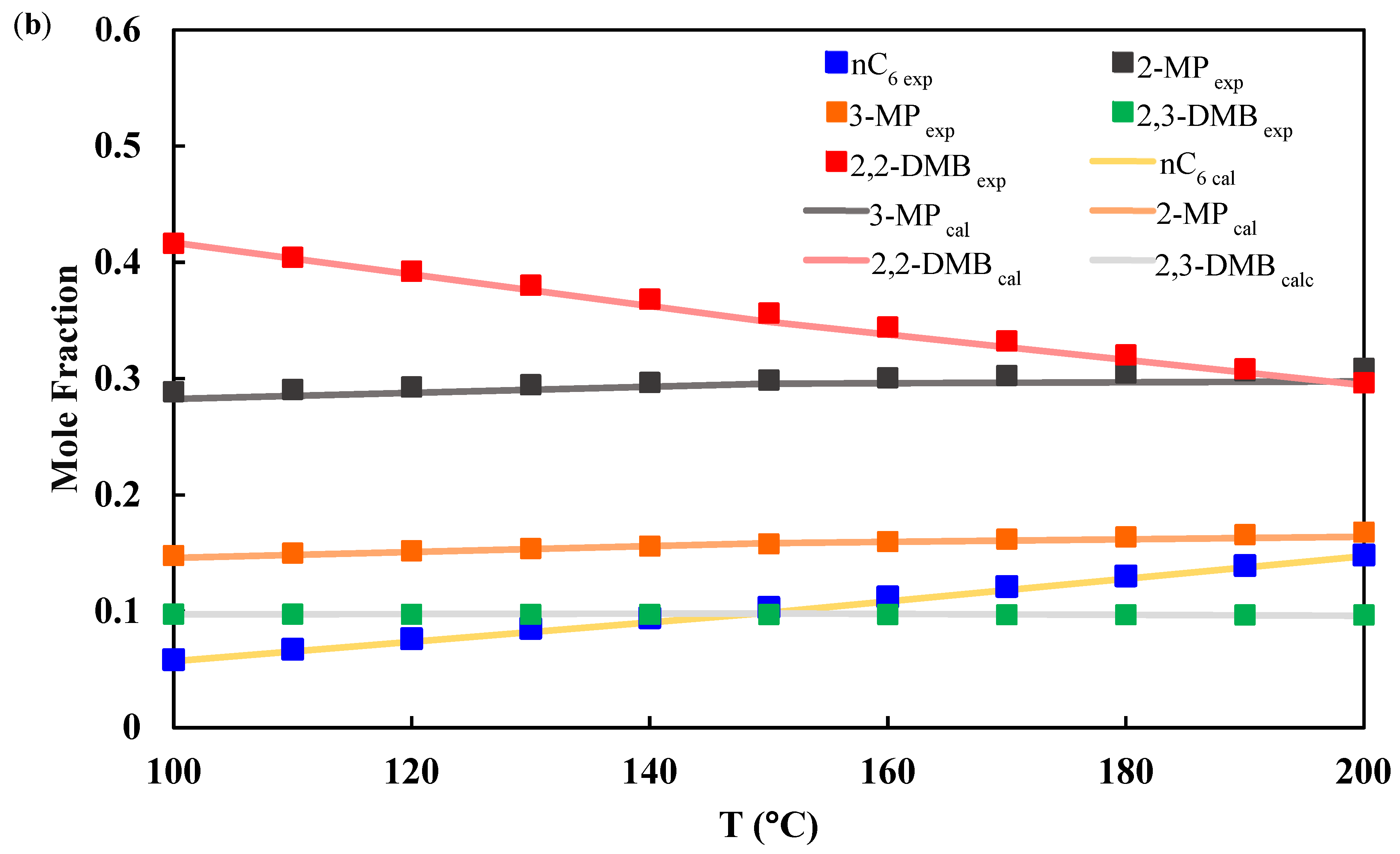
3.1. Chemical Equilibrium

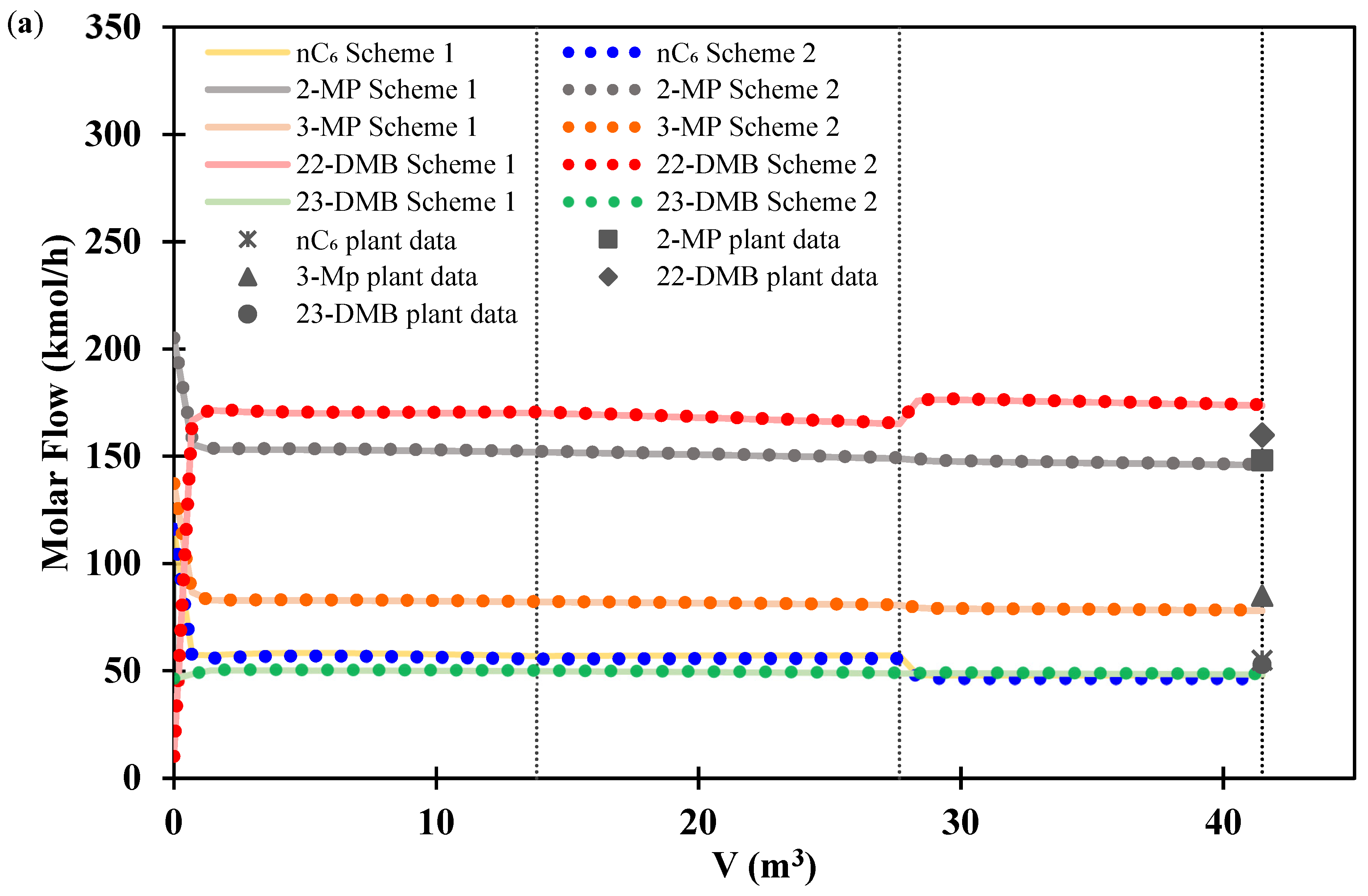
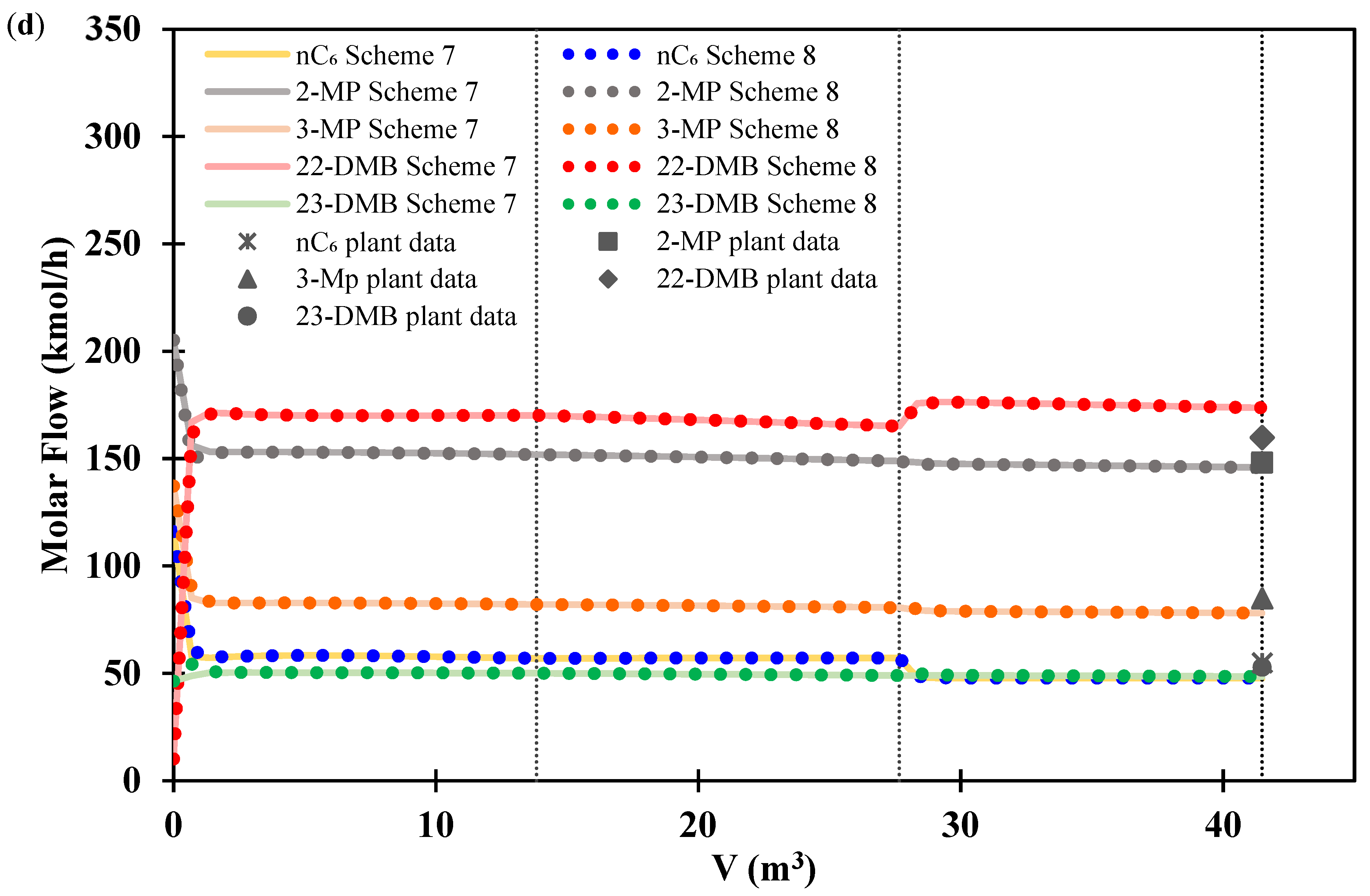
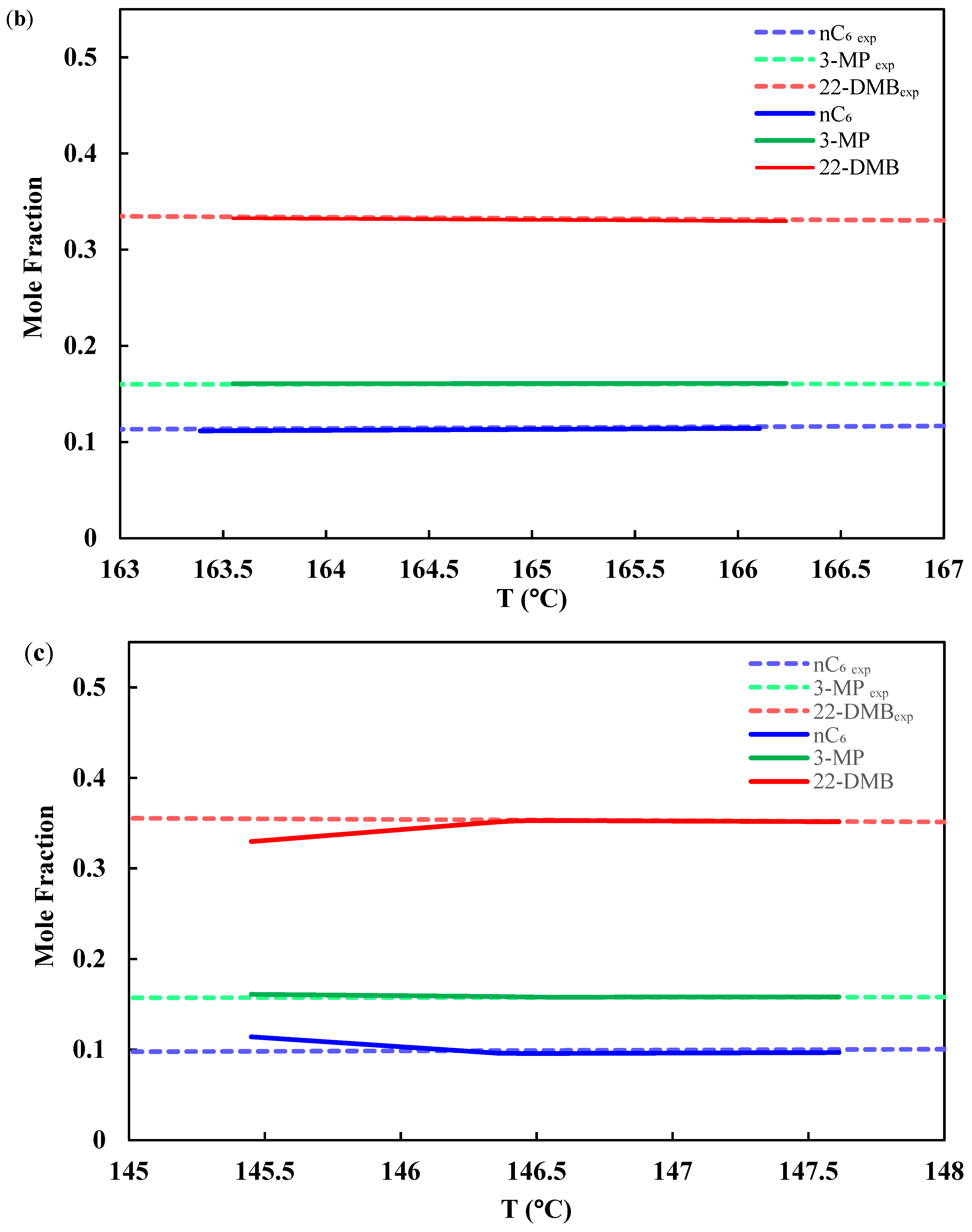
The equilibrium parameter values, Ae and Be for the C₄ and C₅ series, as well as for the reaction schemes of the C₆ series presented in

Table 3. Kinetic and equilibrium parameters of the reaction set.

No.	$\mathbf{A}\left(\frac{\mathbf{m}\mathbf{o}\mathbf{l}}{{\mathbf{m}}^3\mathbf{h}}\right)$	${\mathbf{E}\left(\frac{\mathbf{k}\mathbf{J}}{\mathbf{k}\mathbf{m}\mathbf{o}\mathbf{l}}\right)}^{\mathbf{*}}$	${\mathbf{A}}_{\mathbf{e}}$	${\mathbf{B}}_{\mathbf{e}}$
1	2.1404 × 1015	79,100.00	−2.1384	1166.4
2	3.3047 × 1015	79,411.60	−0.6308	745.10
3	Values of the respective C6 series scheme
4
5
6
7
8	7.8288 × 1014	87,250.67
9	3.3698 × 108	54,405.67
10	1.2296 × 106	31,903.05
11	9.5595 × 1012	80,522.16
12	2.3764 × 1013	75,961.05
13	3.2298 × 109	62,673.40
14	9.3115 × 104	29,091.70
15	1.6746 × 1010	71,126.52
16	7.4853 × 1011	71,437.13
17	3.3165 × 109	71,546.33

* Taken from Diaz-Cervantes et al. [17].

and

Table 4. Kinetic constants and equilibrium parameters of the reactions in the C6 series schemes.

Reaction	$\mathbf{A}\left(\frac{\mathbf{m}\mathbf{o}\mathbf{l}}{{\mathbf{m}}^3\mathbf{h}}\right)$	$\mathbf{E}\left(\frac{\mathbf{k}\mathbf{J}}{\mathbf{k}\mathbf{m}\mathbf{o}\mathbf{l}}\right)$	${\mathbf{A}}_{\mathbf{e}}$	${\mathbf{B}}_{\mathbf{e}}$
$n{C}_6\leftrightarrow 2-MP$	2.0911 × 1016	78,300.00	−2.6386	1580.30
$n{C}_6\leftrightarrow 3-MP$	2.2400 × 1017	86,300.00	−2.9883	1464.30
$\left(2\right){nC}_6\leftrightarrow 2-MP+3-MP$	4.8600 × 1019	80,600.00	−5.6357	3073.50
$n{C}_6\leftrightarrow \mathrm{2,3}-DMB$	2.9142 × 1013	74,921.73	−4.0006	1690.20
$n{C}_6\leftrightarrow \mathrm{2,2}-DMB$	3.4772 × 1015	79,357.62	−4.1394	2285.10
$2-MP\leftrightarrow 3-MP$	9.3100 × 1015	86,300.00	−0.3496	−116.09
$2-MP\leftrightarrow 2,3-DMB$	5.2100 × 1015	81,800.00	−1.3620	109.86
$2-MP+3-MP\leftrightarrow \left(2\right)2,3-DMB$	6.8600 × 1016	81,600.00	−2.3747	335.96
$2-MP\leftrightarrow 2,2-DMB$	9.1100 × 1016	91,800.00	−1.5014	705.26
$3-MP\leftrightarrow 2,3-DMB$	2.2400 × 1017	86,300.00	−1.0125	226.02
$2,3-DMB\leftrightarrow 2,2-DMB$	5.5137 × 1018	89,900.00	−0.1388	594.89

, respectively, were determined following the methodology detailed in Section 2.1.

The validation of this methodology was performed by solving an equilibrium reactor for each hydrocarbon series (C₄ and C₅) and the reaction schemes of the C6 series. A base feed of 150 kmol/h was used for calculations, and the equilibrium compositions were determined for each temperature within a range from 100 to 200 °C.

The model exhibits satisfactory agreement with experimental data for both the C₄ and C₅ series and the studied schemes of the C₆ series. Figure 1 presents the equilibrium reactor modeling results for schemes 1 and 8. The overlap between the calculated curves and the experimental data [20] confirms the validity of the model. Furthermore, in the C₆ series, the individual behavior of each compound can be analyzed while preserving information on the specific distribution of isomers, in contrast to the 2-MP + 3-MP representation [17].

3.2. Isomerization

The three reactors in series in the isomerization process were initially simulated under adiabatic operation using Fortran code, following the procedure described in Section 2.2. However, in the first reactor, a temperature prediction error of 6.72% was observed compared to plant data, probably due to energy losses [17].

The model considers energy losses in the first reactor, which are mainly attributed to its thermal insulation. According to the data reported by Enikeeva et al. [15], none of the studied reactors have a cooling system; therefore, it is not necessary to include the influence of external heating or cooling effects in the model under industrial conditions [24]. Considering heat transfer between the reactor and its surroundings, the lack of detailed information on the construction materials and insulation type prevents accounting for its effect through the heat transfer coefficient, U.

Thus, a non-adiabatic model was adopted, assuming a heat loss of Q = −2.70 × 10⁶ Kj/h [17] in the energy balance, Equation (12), where $Q_n=Q/n$. This consideration was applied to the first reactor for all eight reaction schemes.

In the literature on petroleum refining processes, such as catalytic reforming (CCR) and isomerization, where kinetic parameters are estimated from experimental data at both industrial and laboratory scales, a frequent limitation has been noted: the experimental data available for industrial-scale processes are often scarce and, in most cases, fewer in number than the kinetic parameters required for their modeling [7,11,14,16,27,28,29,30]. Ancheyta-Jufirez and Villafuerte-Macías [30] highlight that, under this condition, the set of estimated values for the kinetic parameters cannot be unique. The challenge of having fewer plant experimental data compared to the number of kinetic parameters required to model petroleum refining processes has been a historical issue.

Despite this difficulty, the simulation of these processes remains a fundamental tool, particularly for the development of applications such as Operator Training Simulation (OTS).

In a nonlinear parameter estimation problem, to avoid potential overfitting, it is necessary for the number of experimental data to be greater than the number of parameters to be determined in the modeling. To ensure that the model does not incur in overfitting, only 16 frequency factors were estimated against a total of 20 plant experimental data [15].

Initially, 16 kinetic parameters corresponding to the frequency factor (A_j) were determined through optimization for Scheme 1, as the activation energy (B_j) values taken from Diaz-Cervantes et al. [17] remained fixed.

The A_j and B_j values for the reactions of the C₄ and C₅ series, as well as for benzene saturation and cracking reactions, were fixed, and subsequently, the predictive performance of the remaining schemes in the C₆ series was evaluated. These parameters are presented in Table 3.

For the reactions in the C₆ series, the values of A_j and E_j were optimized individually for each reaction, independent of the scheme in which they were included. Therefore, the kinetic parameters of a specific reaction can be applied to any combination, provided that the reaction is part of the scheme. Table 4 lists all the reactions used in the eight schemes, along with their corresponding kinetic and equilibrium parameters.

The average prediction error for the eight schemes ranged from 3.18% to 3.34% with respect to molar flows. Schemes 1, 3, 5, and 7 exhibited an error of 3.18%, while schemes 4, 6, and 8 showed an error of 3.19%. Scheme 2 had the highest error at 3.34%. However, the difference between the maximum and minimum values was only 0.16%, which is considered negligible. Figure 2 presents the molar profiles of the C₆ series as a function of cumulative volume for the eight schemes, compared in pairs to facilitate visual analysis. The results indicate that all schemes exhibit the same trend.

As shown in Figure 2, under the specific operating conditions of the case study and the reactor tuning performed through the estimation of nonlinear parameters, the results indicate that the components undergo a reaction primarily at the reactor inlet. This suggests that maximum conversion is achieved rapidly, approximately at 4 m³. Additionally, the same figure reveals a small step between the second and third reactors, which can be attributed to the prior cooling operation, promoting further isomer formation. As can be observed in Figure 2a–c.

Regarding temperature, the eight schemes exhibit an average prediction error of 1.44%. The temperature profile among the three reactors is shown in Figure 3. Since the prediction errors for both molar flows and temperatures are nearly identical, it can be concluded that any of the eight analyzed schemes allow for the accurate modeling of the phenomenon.

As proposed by Díaz-Cervantes et al. [17], it is possible to determine the regions dominated by kinetics and chemical equilibrium through a detailed analysis based on temperature and the sum of the component flows for each series (C₄, C₅, and C₆), compared with equilibrium compositions. In the case of isomerization, based on plant data reported by Enikeeva et al. [15], Díaz-Cervantes et al. [17] establish that, for the C₆ series, the chemical equilibrium region is reached in the first reactor at 162.8 °C and in the third reactor at 146.4 °C, while in the second reactor, chemical equilibrium predominates.

In Figure 4, which presents the analysis for the components n-C6, 3-MP, and 2,2-DMB from Scheme 4, the results of this study are shown to be consistent with previous findings. The kinetic region predominates in the first and third reactors up to approximately 162 °C (Figure 4a) and 146.5 °C (Figure 4c), respectively, while the second reactor remains in equilibrium (Figure 4b).

It is important to emphasize that the model proposed by Díaz-Cervantes et al. [17] is based on three reversible reactions, demonstrating that any reaction scheme that appropriately incorporates equilibrium information allows for a precise and consistent analysis of the process.

The reaction extent profiles for each reaction in the C₆ series vary depending on the specific scheme studied. However, as observed in the molar flow profiles, all schemes lead to the same result, despite differences in the extent profiles. In contrast, for the reactions in the C₄ and C₅ series, as well as for the benzene saturation and cracking reactions, the reaction extent profiles show no variations between the schemes.

4. Conclusions

The results from the eight schemes modeling the C₆ series show that incorporating rigorous chemical equilibrium information into the model leads to virtually identical predictions. The average prediction errors for molar flows range between 3.18% and 3.34%, while for temperature, the error is 1.44% across all schemes. These results confirm the good fit of the model and enable a detailed analysis of the phenomenon with any of the schemes, as long as the reactions considered are sufficient to define the reactor behavior.

Although the linearly dependent schemes provide results similar to the independent ones, it is important to highlight that the independent schemes avoid redundancy in the model and allow for the representation of the C₆ series with fewer reactions, thereby facilitating its solution.

Additionally, modeling the C₆ series using both linearly dependent and independent schemes resulted in a significant reduction in the number of chemical reactions, achieving a decrease of 72.2% and 77%, respectively, compared to the model reported in the literature [15], which considers 18 reactions.

The results obtained indicate that the values of the kinetic constants for the reactions may be unique. That is, regardless of the scheme used among the eight studied for the C₆ series in the kinetic set of the isomerization process analyzed, the values of A_j and E_j for the reactions remain invariable.

References

1. Mammadova, M.; Isayeva, Y.; Agayeva, S.; Zarbaliev, R.; Iskenderova, A.; Imanova, A.; Abasov, S. Isomerization conversion of straight run gasoline, gas gasoline and their mixture on Co/HZSM-5/ZrO2/SO4 composite catalyst. Process. Petrochem. Oil Refin. 2024, 25, 343–352. [Google Scholar] [CrossRef]
2. Awadh, A.; Ammar, S. Synthesis of efficient bifunctional Pt/PWA-Nb2O5 nanocatalysts for catalytic isomerization of n-hexane: Experimental and optimization studies. Case Stud. Chem. Environ. Eng. 2024, 10, 100898. [Google Scholar] [CrossRef]
3. Hassan, N.; Jalil, A.; Twu, L.; Fatah, N.; Hambali, H.; Hussain, I.; Firmansyah, M. Hydroisomerization of n-hexane over metal oxides-loaded fibrous silica catalyst for cleaner fuel production. Int. J. Hydrogen Energy 2023, 48, 20525–20537. [Google Scholar] [CrossRef]
4. Song, Y.; Peng, B.; Wang, R.; Han, L.; Zhao, W.; Wang, L.; Lin, W. One-step desilication-recrystallization towards enhanced diffusion for Ni/ZSM-5-catalyzed n-hexane hydrogenative isomerization. J. Chem. Eng. 2023, 476, 1385–8947. [Google Scholar] [CrossRef]
5. Dzhikiya, O.; Smolikov, M.; Belopukhov, E.; Yablokova, S.; Doronin, A.; Gulyaeva, T.; Belyi, A. A study of fluorine-containing catalysts based on MOR and BEA zeolites in isomerization of n-hexane. AIP Conf. Proc. 2020, 2285, 020005. [Google Scholar]
6. Bolton, A.; Lanewala, M. A mechanism for the isomerization of the hexanes using zeolite catalysts. J. Catal. 1970, 18, 1–11. [Google Scholar] [CrossRef]
7. Ahmed, A.M.; Jarullah, A.T.; Abed, F.; Mujtaba, I. Modeling of an industrial naphtha isomerization reactor and development and assessment of a new isomerization process. Chem. Eng. Res. Des. 2018, 137, 33–46. [Google Scholar] [CrossRef]
8. Said, M.; Ahmed, T.; Moustafa, T. Predictive Modeling and Optimization for an Industrial Penex Isomerization Unit: A Case Study. Energy Fuels 2014, 28, 7726–7741. [Google Scholar] [CrossRef]
9. Cull, N.; Brenner, H. Applying Nonlinear Regression to Kinetics of Hexane Isomerization. Ind. Eng. Chem. 1961, 53, 833–836. [Google Scholar] [CrossRef]
10. Evering, B.; Waugh, R. Catalytic Isomerization of Isomeric Hexanes. Ind. Eng. Chem. 1951, 43, 1820–1823. [Google Scholar] [CrossRef]
11. Volkova, G.; Reshetnikov, S.; Shkuratova, L.; Budneva, A.; Paukshtis, E. n-Hexane skeletal isomerization over sulfated zirconia catalysts with different Lewis acidity. Chem. Eng. J. 2007, 134, 106–110. [Google Scholar] [CrossRef]
12. Koncsag, C.; Tutun, I.; Safta, C. Study of C5/C6 isomerization on Pt/H-zeolite catalyst in industrial conditions. Ovidius Univ. Annal. Chem. 2013, 22, 102–106. [Google Scholar]
13. Adžamić, T.; Mužic, M.; Adžamić, Z.; Sertić Biond, K. Isomerization of n-Hexane on Pt/SO4-ZrO2. GOMABN 2011, 50, 12–21. [Google Scholar]
14. Chekantsev, N.; Gyngazova, M.; Ivanchina, E. Mathematical modeling of light naphtha (C5, C6) isomerization process. Chem. Eng. J. 2014, 238, 120–128. [Google Scholar] [CrossRef]
15. Enikeeva, L.; Faskhutdinov, A.; Koledina, K.; Faskhutdinova, R.; Gubaydullin, I. Modeling and optimization of the catalytic isomerization of the pentane hexane fraction with maximization of individual high-octane components yield. React. Kinet. Mech. Catal. 2021, 133, 879–895. [Google Scholar] [CrossRef]
16. Faskhutdinov, A.; Faskhutdinova, R.; Arefyev, I.; Enikeeva, L. Numerical simulation of the catalytic process of isomerization of pentane-hexane cut. J. Phys. Conf. Ser. 2019, 1368, 042016. [Google Scholar] [CrossRef]
17. Diaz-Cervantes, D.K.; Castro-Agüero, A.; López-Medina, F.; Ortíz-Arroyo, A.; Pérez-Villaseñor, F.; Medina-Velázquez, D.Y.; Elías-Domínguez, A. A short reaction kinetic set for modeling the isomerization process considering rigorous chemical equilibrium. Next Res. 2025, 2, 100173. [Google Scholar] [CrossRef]
18. Strang, G. Introduction to Linear Algebra, 5th ed.; Wellesley-Cambridge Press: Wellesley, MA, USA, 2022. [Google Scholar]
19. Pines, H.; Kvetinskas, B.; Kassel, L.; Ipatieff, V. Determination of Equilibrium Constants for Butanes and Pentanes. J. Am. Chem. Soc. 1975, 67, 631–637. [Google Scholar] [CrossRef]
20. PENEX UOP, Operation Manual. 1995.
21. Smith, J.; Van Ness, H.; Abbott, M.; Swihart, M. Introduction to Chemical Engineering Thermodynamics, 8th ed.; McGraw-Hill Education: New York, NY, USA, 2018. [Google Scholar]
22. Tiscareño, L.F. ABC Para Comprender Reactores Químicos con Multireacción, 1st ed.; Reverté: Tampico, Mexico, 2008. [Google Scholar]
23. Walas, S. Phase Equilibria in Chemical Engineering, 1st ed.; Butterworth: Boston, MA, USA, 1985. [Google Scholar]
24. Fogler, S.H. Elements of Chemical Reaction Engineering; Michigan Prentice Hall: Boston, MA, USA, 2020. [Google Scholar]
25. Honeywell. UniSim Design Suite R500TM; Honeywell: Charlotte, NC, USA, 2024. [Google Scholar]
26. Stewart, W.; Caracotsios, M.; Sorensen, J. Non-Linear Estimation Parameters Using the GREG Program; Department of Chemical Engineering, University of Wisconsin-Madison: Madison, WI, USA, 1990. [Google Scholar]
27. Chuzlov, V.A.; Chekantsev, N.V.; Ivanchina, E.D. Development of Complex Mathematical Model of Light Naphtha Isomerization and Rectification Processes. Procedia Chem. 2014, 10, 236–243. [Google Scholar] [CrossRef]
28. Chuzlov, V.A.; Ivanchina, E.D.; Chekantsev, N.V.; Molotov, K.V. Efficiency improvement of the light gasoline fractions isomerization by mathematical modeling. Procedia Eng. 2025, 113, 131–137. [Google Scholar] [CrossRef]
29. Padmavath, G.; Chaudhuri, K.K. Modelling and Simulation of Commercial Catalytic Naphtha Reformers. Can. J. Chem. Eng. 1997, 75, 930–937. [Google Scholar]
30. Ancheyta-Jufirez, J.; Villafuerte-Macias, E. Experimental validation of a kinetic model for naphtha reforming. Stud. Surf. Sci. Catal. 2001, 133, 615–618. [Google Scholar]
Figure 1. Chemical equilibrium compositions for reaction Schemes 1 (a) and 8 (b) of the C6 series.
Applsci 15 04429 g001aApplsci 15 04429 g001b
Figure 2. Molar flow profiles in the three reactors for Schemes 1-2 (a), 3-4 (b), 5-6 (c), 7-8 (d) –8 of the C6 series.
Applsci 15 04429 g002aApplsci 15 04429 g002bApplsci 15 04429 g002c
Figure 3. Temperature profile along the three reactors of the isomerization process.
Applsci 15 04429 g003
Figure 4. Mole fraction of the C6 series C6 (c) C 6 , i / C 6 , k as a function of temperature in the first (a), second (b), and third (c) reactors of scheme 4.
Applsci 15 04429 g004aApplsci 15 04429 g004b