Abstract
While autonomous vehicles have the potential to mitigate risks associated with dangerous driving behaviors, the safety and stability of autonomous driving technology in real-world applications still require comprehensive tests. Scenario-based virtual simulation testing has emerged as a crucial approach for testing autonomous vehicles, especially in critical scenarios under complex environments, such as merging scenarios at roundabouts with unique traffic features. However, the lack of high-risk scenarios in the real-world traffic domain presents challenges for simulation tests. To address these challenges, this study proposes a scenario generation framework for complex roundabout environments, focusing on merging areas, which is driven by trajectory data and employs generative deep learning techniques to create adversarial hazardous scenarios. Specifically, leveraging real trajectory data from roundabouts, the framework utilizes a time series generative adversarial network (TimeGAN) to generate realistic safety-critical driving trajectories. By creating specific hazardous scenarios, this strategy broadens the library of test scenarios and speeds up the testing process for autonomous vehicles. The significance of the scenarios produced is proven using Simulation of Urban Mobility (SUMO) and CARLA simulation, confirming their necessity in autonomous driving testing. The TimeGAN model effectively captures the spatial–temporal features of merging scenarios, generating high-quality data that enhance the testing scenario library. Findings of this study contribute to solving the problem of scarcity of critical scenarios in virtual testing and accelerate the testing procedure for self-driving automobiles.
1. Introduction
Autonomous vehicles have the potential to mitigate risks associated with dangerous driving behaviors, providing a key solution for enhancing road safety. However, the safety associated with autonomous vehicles should not be ignored. Since 2014, the California Department of Motor Vehicles (DMV) has reported 704 collisions involving autonomous vehicles [1]. According to the statistics, there has been an annual increase in the number of accidents since one was reported in 2014, with a peak of 105 in 2019. Only in 2020, the number of accidents dropped to 44 as a result of the COVID-19 pandemic. However, in 2021, the number of accidents resumed its upward trend. This trend has made the exploration of the practical application and safety of autonomous driving technology an important topic of research and public concern. Safety remains the primary issue that autonomous vehicles must address before they can be widely adopted for commercial purposes [2]. Therefore, how to conduct comprehensive tests on the autonomous driving system, test as diverse driving scenarios as possible before putting them into use, and discover existing safety problems are the current challenges.
One of the current major test methods is the road test, but it is time-consuming, inefficient, and costly. Similar low-risk scenarios make up the majority of real road test scenarios, whereas less frequently occur more hazardous circumstances with significant testing value. To guarantee sufficient safety of autonomous vehicles through real-world road testing, it will be expensive and take a long time. Researchers have suggested that approximately 99% of testing and verification work should be conducted in virtual environments [3], with only about 0.9% taking place on actual test sites. As a result, scenario-based virtual simulation testing can lessen the workload associated with field testing while better satisfying the needs for extensive and effective autonomous driving testing.
At present, testing scenarios can be classified into typical scenarios and edge scenarios according to the requirements. Typical scenarios are generally used for routine functional testing of autonomous driving systems, typically selected from real traffic data as representative test cases, but they cannot cover all real-world conditions. For testing autonomous vehicles, it is crucial not only to focus on the safety of various vehicle functions in normal driving scenarios, but also to emphasize the vehicle’s ability to safely navigate challenging testing scenarios. Selecting high-risk scenarios from numerous complex traffic situations has become a focal point [4,5]. Thus, edge scenarios complement typical scenarios and are described as low-probability event scenarios that are difficult to handle, lying between the boundaries of danger and safety. At the same time, autonomous driving scenarios exhibit high levels of uncertainty, with a complexity that is difficult to exhaustively cover. To enhance scenario coverage, it is necessary to evolve new derivative scenarios from real traffic data. Currently, methods for generating such critical scenarios include optimization search-based generation [6,7,8], reinforcement learning-based generation [9,10,11], importance sampling-based generation [12,13,14], and deep-learning-based generation [15,16,17]. However, whether the characteristics of derived scenarios are consistent with real traffic data remains unknown. It is possible to generate scenarios that do not exist in the real world, so derived scenarios need to be validated for authenticity before use.
As a primary component of scenarios, the driving states reflected by vehicle trajectories can be utilized to simulate the dynamic changes in driving behaviors, thereby supporting the construction of diverse and realistic testing scenarios. However, since challenging scenarios are very rare in the actual traffic field, resulting in difficulties in obtaining sufficient safety-critical trajectories by means of data collection, most of the naturalistic driving data collected are safe [18]. Considering that trajectories involving high-risk confrontational behavior between surrounding vehicles (called safety-critical trajectories) are integral to simulation testing, a generative approach to obtaining vehicle trajectories is used to address this issue [19]. Deep learning methods can model key trajectory data from naturalistic driving trajectories, capturing driving patterns within the dataset and generating uncovered, realistic, and safety-critical driving trajectories. These novel scenarios evolved from existing time series traffic trajectory data and greatly enrich the diversity of the test scenario library samples, improving test coverage.
The selected research object in this study, the roundabout, is a type of complex and critical scenario. Identifying challenging edge scenarios within it and deriving them should be a focus of attention for autonomous driving. The uniqueness of roundabouts at intersections lies in their connection to surrounding roads through circular paths, with vehicles traveling within the roundabout having higher priority. These arrangements help reduce accident rates and the severity of accidents. However, for multi-lane roundabouts, the traffic conditions are complex, and frequent lane changes by vehicles entering and exiting can create conflict points, leading to increased risk in merging and diverging zones. Moreover, vehicles traveling within the roundabout experience constantly changing speeds and acceleration directions. The use of roundabouts is becoming increasingly common in many countries, and safety issues are becoming more widespread. However, research on key areas of safety at roundabouts, like the merge zones, has not received the attention it deserves, especially in the area of scenario generation.
Based on the analysis above, this study proposes a research framework for high-risk scenarios in roundabout environments. The hazardous scenarios are simplified to the trajectories of interacting vehicles. A generative model that combines autoregressive modeling and adversarial network learning captures the characteristics of vehicle interactions, preserves the dynamic information of temporal trajectories, and derives and generalizes more key scenarios for autonomous driving tests. Additionally, the quality of the derived key roundabout scenarios is assessed from three perspectives: diversity, similarity, and authenticity. Finally, a simulation model is established to test the generated scenarios, including a new simulation method that validates the applicability and importance of the generated scenarios for autonomous driving tests. The following are this study’s primary contributions:
- (a)
- To preserve the characteristics of vehicle operation within roundabouts, a modified two-dimensional time-to-collision (MTTC) model is used to identify high-risk scenarios in merging areas and to pinpoint interacting vehicles that may pose collision risks. To enhance the efficiency of derivation and simplify scenario information, the focus of the study is shifted to driving trajectories, making the method more generalizable and applicable.
- (b)
- A time series generative network is introduced to generate key scenarios at roundabouts, effectively capturing the motion characteristics of interacting vehicle pairs and the temporal features of sequential trajectories. The evaluation metrics for the produced outcomes are improved, verifying the diversity of the derived scenarios, their similarity to real-world situations, and the probability that they would materialize in the real world from different perspectives.
- (c)
- A simulation experiment scenario is established, and a new test method is developed that specifies the trajectory of one vehicle and the starting point of another to assess the risk of interaction between the vehicles.
The following is the structure of this paper: Section 2 offers an overview of the literature. Section 3 describes the research methods, including data processing, model generation, evaluation of generated scenarios, CARLA simulation (an open urban driving simulator), and Simulation of Urban Mobility (SUMO). Section 4 presents the results and discussion, and the paper ends with conclusions in Section 5. For the sake of clarity and ease of reference, all acronyms used throughout this manuscript are defined in the following Table 1.

Table 1.
The definitions of the acronyms.
2. Literature Review
2.1. Safety Research at Roundabouts
Compared to conventional intersections, roundabouts have the advantage of reducing the frequency and severity of traffic crashes, as well as contributing to the efficiency of road traffic [20]. However, when navigating a multi-lane roundabout, cars must switch lanes several times as they enter and depart the traffic circle. This results in multi-lane changes having more conflict points than single-lane changes, increasing the likelihood of collisions [21].
In roundabout safety research, scholars have conducted in-depth analyses of conflict occurrence locations. Although the traffic law stipulates that vehicles about to enter the traffic circle have to give way to vehicles already inside the traffic circle, in practice, there still exists a right-of-way competition problem for vehicles traveling in these two different lanes, and the danger of vehicles passing by the traffic circle’s entrance is higher. Al-Ghandour et al. [22] conducted simulation studies and found that the conflict frequency in the merging area is significantly higher than the rest of the approach or diverging areas at roundabouts. Additionally, Guo et al. [23] emphasized the importance of the merging area in overall performance, as it serves as a bottleneck for the capacity of the roundabout.
The most common research tool used in studies on safety is surrogate safety measures (SSM). Time-to-collision (TTC) metrics have been widely used as the most common measures in traffic engineering, road safety, and other fields [24,25,26]. However, the calculation and definition of the traditional TTC metrics are too simplistic, which is better suited for scenarios where motion is concentrated in one direction. Therefore, the MTTC has been proposed to more accurately capture the safety characteristics of vehicle operations under real road conditions [27]. Charly et al. [28] also utilized the MTTC as a collision metric, taking into account both lateral and longitudinal distances. The results indicated that the MTTC has better predictive ability for collision risks in real-world scenarios. Considering that vehicles’ movements within roundabout scenarios involve curved trajectories, dissecting the motion into lateral and longitudinal is more accurate. In summary, this article selects the merging area of roundabouts as the research object, introducing the MTTC metric to analyze the safety of this area and extract hazardous scenarios.
2.2. Research on Vehicle Trajectory Generation
In recent years, data augmentation techniques have been proposed to address datasets with insufficient data, particularly in the context of machine learning. As a new generation of artificial intelligence technologies advances, exemplified by deep neural networks, an increasing number of scholars are beginning to explore the use of deep learning methods for scenario derivation. This approach has become a promising paradigm for deriving edge scenarios beyond traditional theoretical search methods. As a typical unsupervised data augmentation technique, the GAN has a very strong ability to generate realistic data and fake the truth, because it contains the properties of both generative and discriminate networks [29]. This has led to its widespread use in areas such as image enhancement, video generation, text generation, and other fields.
The development of GAN models has indeed opened promising avenues for generating hazardous scenarios based on deep learning, addressing the lack of dangerous scenarios in naturalistic driving databases. Vehicle trajectory data, which include precise information on the vehicle’s position, speed, and acceleration at each moment, provide rich details for describing dynamic traffic scenarios. The construction of test scenarios in simulation testing requires a critical trajectory to provide information and reflect whether there is adversarial behavior in traffic environments. Therefore, the generation of hazardous scenarios can be considered by using advanced machine learning algorithms to train and learn the generation of dangerous traffic vehicle trajectories directly from existing databases [30]. Alternatively, the parameter space of the scenario can be expanded by generating samples that do not exist in the scenario library through a data-driven approach [31].
However, the complex relationships between the attributes and temporal characteristics of consecutive points in time series, such as trajectories, pose an additional challenge for generative models. As a relatively new field for GAN research, there is a significant amount of work being done to develop models capable of generating high-quality, diverse, and specific time series data. Particularly in the finance and medical industries, models such as Noise Reduction GAN [32] and Quant GAN [33] have been proposed, which can capture the dependencies in continuous time series data. The superiority of these methods has been confirmed in studies involving time series data with fewer features, such as stocks. However, their effectiveness in generating trajectory data still requires further research.
In the field of trajectory research, many researchers use GAN models to predict motion trajectories [34,35]. Tang and Salakhutdinov [36] focused on the definition and generation of latent codes, aiming to solve the prediction of driving trajectories in scenario-based traffic environments. Some researchers have also begun to explore trajectory generation. Krajewski et al. [30,31] have designed vehicle trajectory generation models based on GAN and VAE, which can generate new lane-changing trajectories without the need for labeled data. Andreas et al. [37] have proposed a deep learning framework driven by real driving data to generate driving trajectories of varying lengths. This framework employs recurrent conditional generative adversarial networks (RC-GANs), which can flexibly generate driving trajectories of variable lengths [38]. It can be found that the generation of vehicle trajectories based on natural driving data with the purpose of generating more scenarios and including temporal features receives less attention. While some researchers have begun to explore the generation of vehicle trajectories using deep learning, their focus has largely been on scenarios such as highways. These scenarios are characterized by straight roads and fewer features in vehicle trajectories. However, roundabout scenarios, where vehicle driving characteristics are more numerous and complex, have not received sufficient attention. To address this gap, this paper introduces a time series generative adversarial network (TimeGAN) to study vehicle trajectories in key roundabout scenarios [39]. TimeGAN is a new framework that generates time series with temporal dynamics by combining more controllable supervised learning techniques with conventional unsupervised GAN training methods.
3. Methodology
3.1. Research Framework
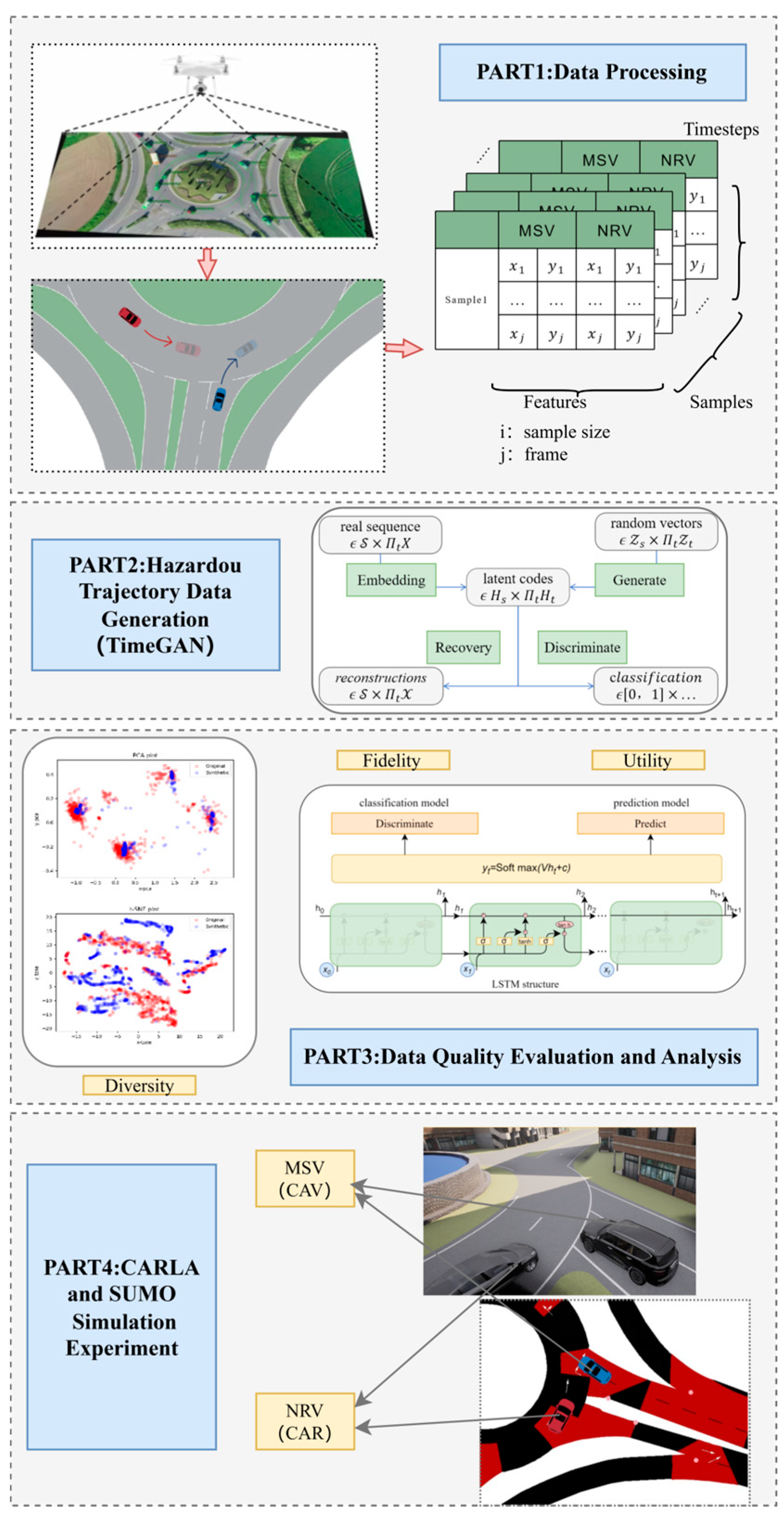
The research framework of this study consists of four main parts, as shown in Figure 1: (1) Data processing, which introduces the extraction of merging scenarios from the RounD dataset and the preprocessing of raw data to obtain basic information on interacting vehicle pairs and hazardous scenarios. (2) Data generation: this part describes the structure of the TimeGAN model and the method of data generation. (3) Data evaluation: the generated data are evaluated from three perspectives, and their respective metrics are proposed in this section. (4) Simulation testing: the last section utilizes the Simulation of Urban Mobility (SUMO) and CARLA platforms to establish a simulation scenario of a roundabout and tests the generated hazardous scenarios to verify the effectiveness of the dangerous trajectories.
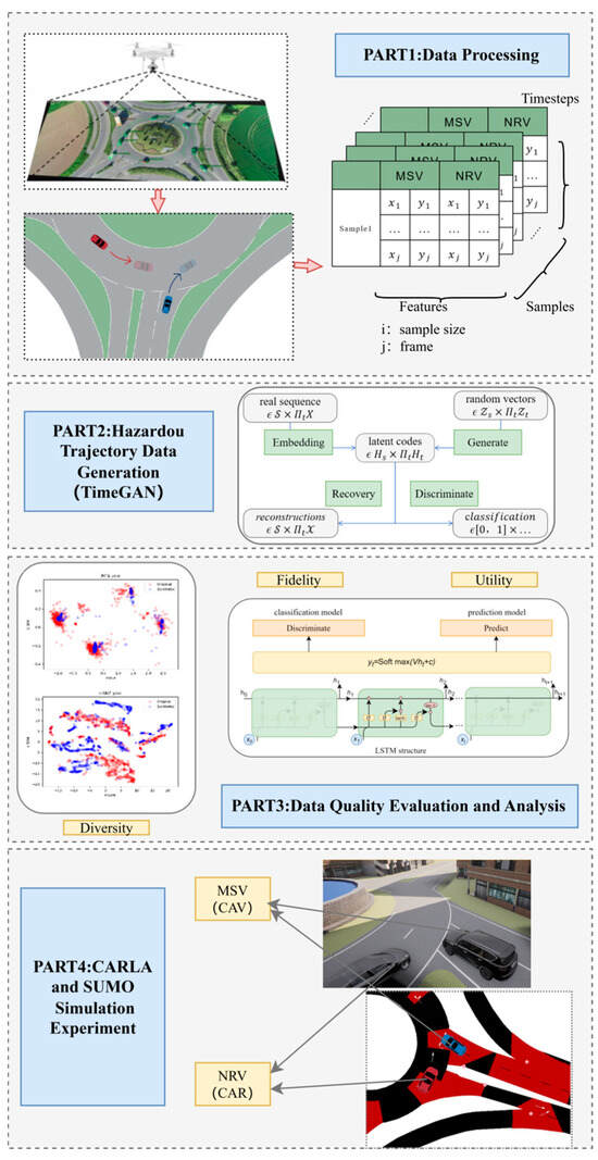
Figure 1.
Research framework.
3.2. Data Processing
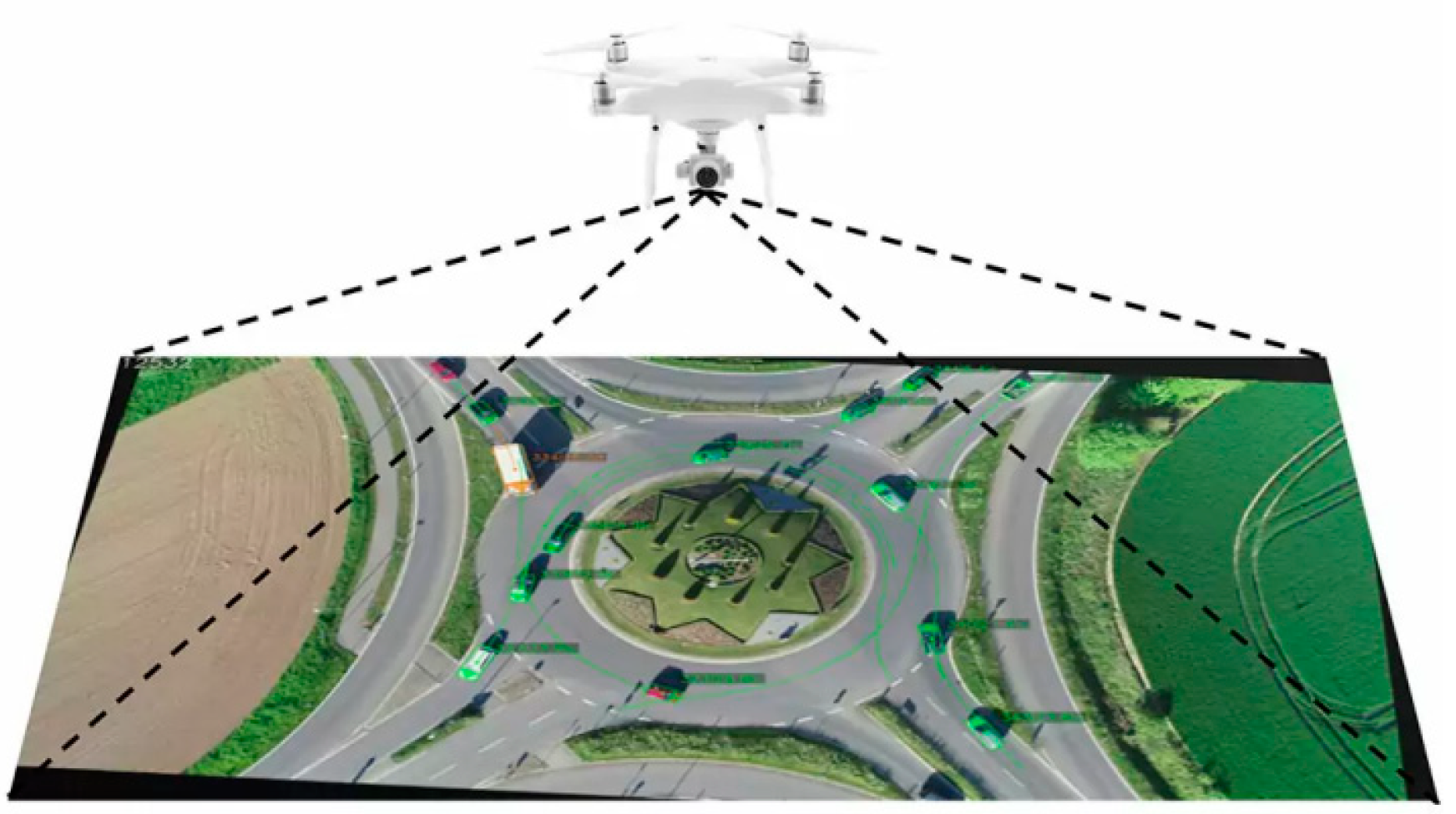
The RounD dataset from RWTH Aachen University in Germany provided the data used in this investigation [40]. This dataset records the trajectories and their types of road users at three separate sites by using drones at a collection frequency of 25. Utilizing state-of-the-art computer vision algorithms, the trajectory position errors are typically less than 10 cm. The roundabout dataset provides four files for every record: a segment image, a file that describes the location where the recording was made, a file that gives a summary of the recorded vehicle trajectories, and a file describing the trajectories. The detailed data include vehicle IDs, timestamps, vehicle positions both longitudinally and laterally, speeds, accelerations, headings, and so on. As depicted in Figure 2, a multi-lane roundabout with a dual-lane entrance and a dedicated right-turn lane was selected from the roundabout dataset. Trajectory data spanning a total of 6 h during different time periods from Tuesday to Thursday were extracted, with a total of approximately 13,000 vehicles.

Figure 2.
Data collection segments of the RounD dataset [40].
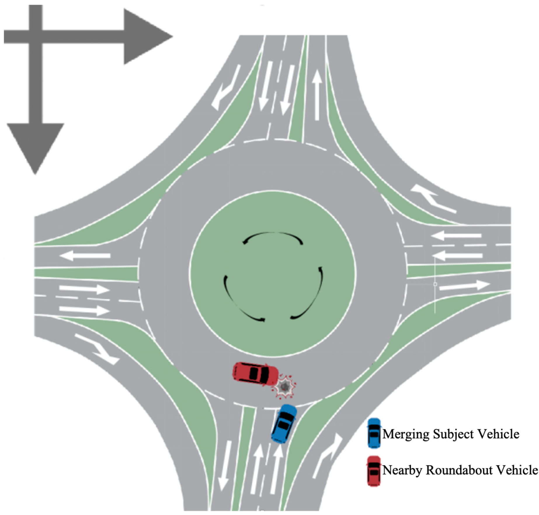
Based on the aforementioned roundabout dataset, vehicle trajectories under merging scenarios were further extracted. During the merging process, the driver prepares to turn right in advance, adjust their driving speed, and steer clear of objects that could obstruct their path, so that the vehicle can safely drive into the roundabout. In this study, an interacting vehicle pair consisting of two vehicles was taken into consideration, as shown in Figure 3. The vehicle attempting to merge into the roundabout was designated as the merging subject vehicle (MSV), which is depicted in blue. This vehicle was the primary focus of our study, as it navigates the complexities of entering the roundabout. The nearby roundabout vehicle (NRV) was identified as the vehicle circling the roundabout closest to the MSV, and it is highlighted in red. This particular vehicle was selected because it poses the highest potential collision risk to the MSV during the merging maneuver.
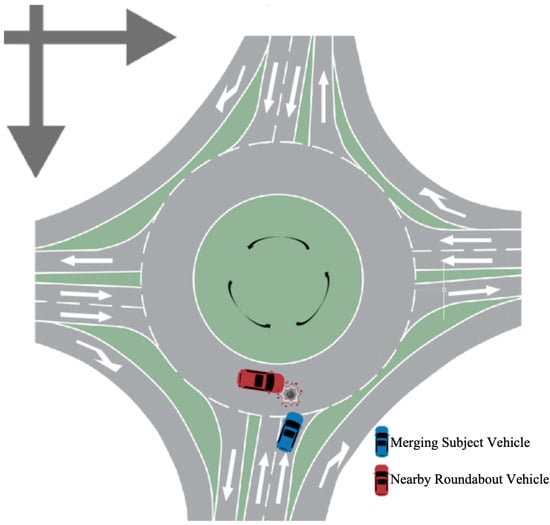
Figure 3.
Description of interactive vehicle pairs in the merge scenario.
Each vehicle entering the roundabout with a risk can find a corresponding vehicle inside the roundabout that poses a significant collision risk. The two vehicles together form a dangerous interaction pair.
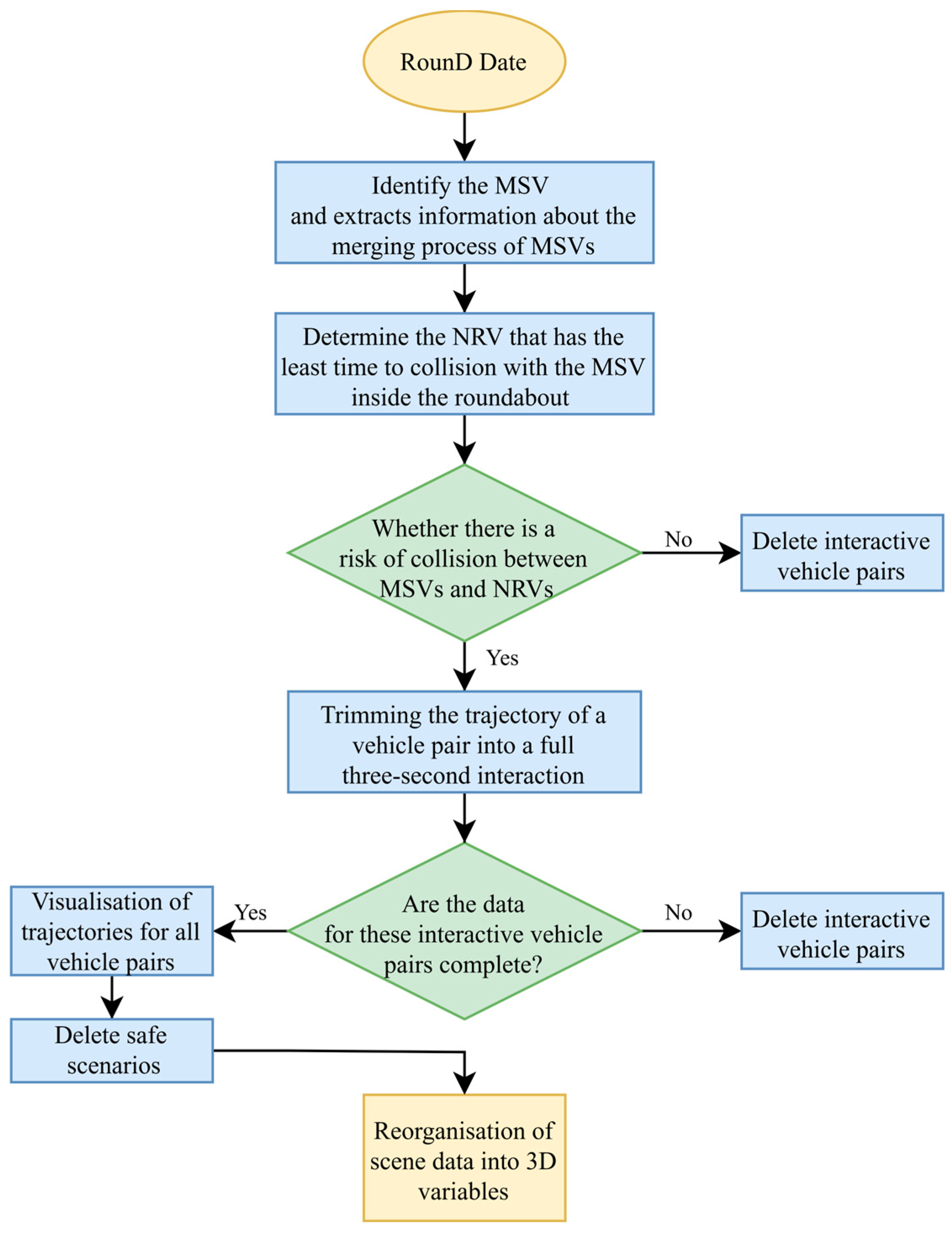
The roundabout merging critical hazard scenario was combined with the fundamental information of the interacting vehicle pair and 3 s of trajectory data, resulting in a complete, continuous, and uninterrupted trajectory data of the two vehicles. The details of the data processing and extraction are depicted in Figure 4. The first step involved identifying the MSV, which is the vehicle attempting to merge into the roundabout. Detailed information about the merging process of the MSVs was extracted. This included data on speed, acceleration, steering angles, and other relevant parameters. Next, the system identified the NRV that has the least time to collision with the MSV inside the roundabout. The workflow then evaluated whether there is a risk of collision between the MSVs and CVs. If no risk was detected, the interactive vehicle pairs were deleted from further analysis. For vehicle pairs identified as having a collision risk, the trajectories were trimmed to include only a full three-second interaction. This trimming ensured that the data analyzed focused on the critical moments leading up to potential collisions, providing a detailed view of the interaction dynamics. After trimming, the system checked if the data for these interactive vehicle pairs were complete. Incomplete datasets were deleted to maintain the quality and reliability of the analysis. If the datasets were complete, the trajectories for all vehicle pairs were visualized. Following this, safe scenarios were deleted, further refining the dataset to include only those scenarios that were critical for safety analysis. The final step involved reorganizing the scene data into 3D variables. More detailed criteria and content are described below.
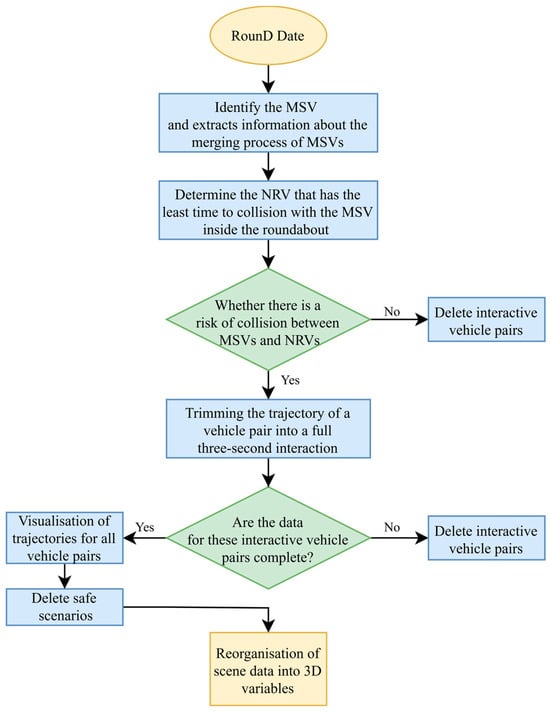
Figure 4.
RounD data processing and extraction process.
3.2.1. Determining the Merging Subject Vehicle
There are two limitations that determine the identification of a vehicle entering a roundabout: (1) At the time , the vehicle remains in the roundabout’s entry lane, meaning the distance between the center of the vehicle and the center of the roundabout is greater than or equal to the radius of the roundabout. (2) At the next time , the distance between the vehicle and roundabout is less than the roundabout’s radius. The two constraints are shown in Equations (1) and (2):
where R is the radius of the roundabout and is the distance between the center of the vehicle and the center of the roundabout at the moment . Moment is considered as the critical moment merging into the roundabout. According to the previous studies, the whole merging process was defined as a time interval of four seconds in total, two seconds before and two seconds after the critical moment.
3.2.2. Extracting Interactive Vehicle Pairs
After identifying all merging vehicles, it was necessary to determine the specific interacting vehicle (RSV), which is defined as the vehicle that has the highest conflict possibility with the MSV during its merging process. Firstly, the global frame was used to find all surrounding vehicles that were present at the same moment as the MSV and then identify RSVs among these vehicles. To quantify the potential conflict, the TTC metric was applied in this study. However, the conventional TTC index is not suitable for roundabout safety evaluation due to the particular structure and complexity of roundabouts. Unlike the straightforward one-dimensional method, conflicts at roundabouts are characterized in two dimensions. Conflict between the MSV and NRV was divided into two dimensions of horizontal X and vertical Y directions. The modified two-dimensional TTC (MTTC) was introduced to identify conflicts, and the calculation formulas are as follows:
where and are the coordinate vectors of the two vehicles, while and are the velocity vectors of the two vehicles, respectively. When the acceleration difference between the two vehicles is zero, the MTTC is determined by the relative speed and distance between the two vehicles. Specifically, it is calculated as the difference in distance divided by the difference in speed. Sometimes, the vehicles’ motion states make a collision impossible, for example, the leading vehicle is moving faster than the following vehicle, or they are moving apart. To represent this scenario, where no collision is possible, the MTTC is defined as infinity. This indicates that the vehicles will not collide under their current motion states. The last possibility is the scenario where the vehicles are on a trajectory that will result in a collision at some point in the future. The MTTC in this case is defined as the time remaining until the closest approach to collision, assuming the vehicles continue to move in their current states. This represents the minimum time before a potential collision occurs if the vehicles maintain their current trajectories. From the formula, it is evident that the MTTC not only accounts for the longitudinal time to collision but also incorporates lateral dynamics. This two-dimensional approach enables a more precise prediction of potential collision risks, especially in complex traffic scenarios like roundabouts, where both forward and side movements are critical. Thus, the MTTC provides an advantage in assessing safety in such intricate environments. So, we calculated the MTTC of the MSV and all surrounding vehicles throughout the merging process. The moment with the smallest MTTC was identified as the most dangerous moment.
3.2.3. Screening for High-Risk Interaction Scenarios
In previous studies, the scenario with a TTC smaller than 3 s was considered as hazardous. Therefore, in this study, vehicle pairs where the MTTC between the MSV and NRV at the most dangerous moment was smaller than 3 s were defined as dangerous vehicle pairs. In order to standardize the scenario length and adapt to the input dimensions of the GAN model, it was necessary to unify the time steps. The trajectory data of dangerous vehicle pairs for the 2 s before and 1 s after the most dangerous moment (a total of 3 s) were combined to form a dangerous scenario. This three-second window, capturing the motion states of both vehicles, collectively formed what we defined as a roundabout merging high-risk scenario in this study.
The original RounD trajectory data contain redundant information, such as speed, in the global coordinate system, and excessive features can affect the convergence and performance of the TimeGAN model. In this study, only the coordinates were selected as basic features because other features, such as speed and acceleration, can be derived from coordinates. Therefore, the horizontal and vertical coordinates of the two vehicles forming the vehicle pair (MSV and NRV) were used as model inputs. In cases where data for certain vehicles were missing, leading to incomplete data, such scenarios were excluded. After excluding scenarios where vehicle trajectory data were missing, a total of 1747 dangerous scenarios were screened out.
3.2.4. Visualization and Grouping
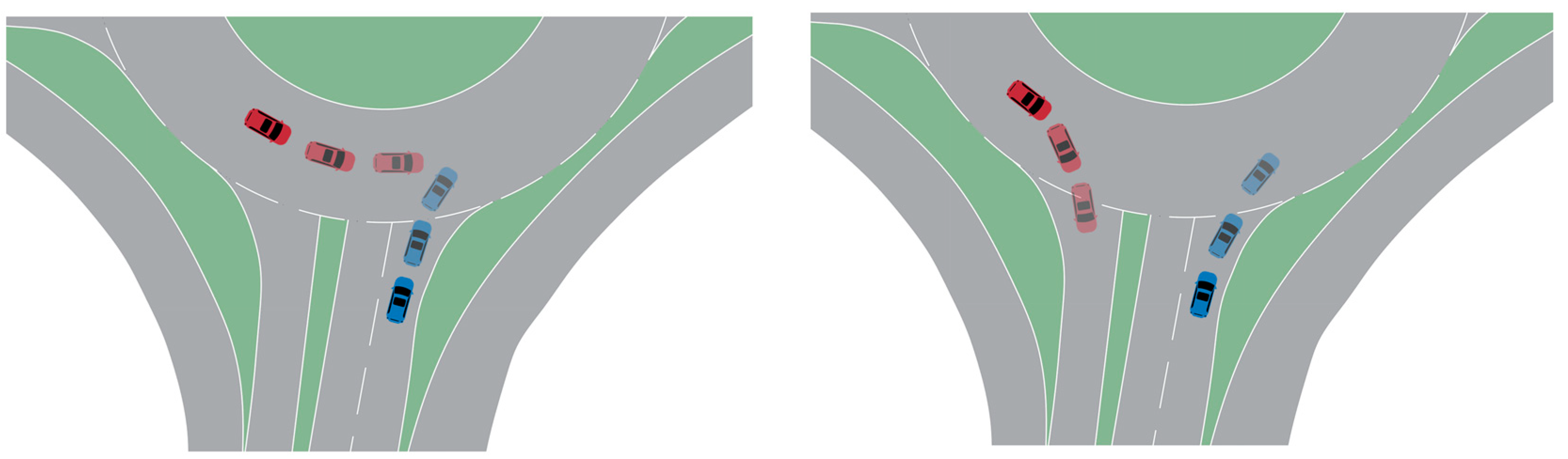
After visualizing all scenarios, it was observed that based on the trajectories of the NRV, they could be divided into two main categories. As shown in Figure 5, one category was where the NRV continued to drive around the roundabout, as in Figure 5a, while the other category was where the NRV exited the roundabout, as in Figure 5b. Considering there were no conflict points between vehicles leaving and entering the roundabout, these 706 sets of sample scenarios, as shown in Figure 5b, were excluded, leaving 1041 dangerous scenario samples for further research.
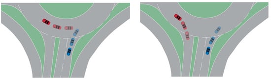
Figure 5.
Scenario visualization classification.
3.2.5. Data Reconstruction
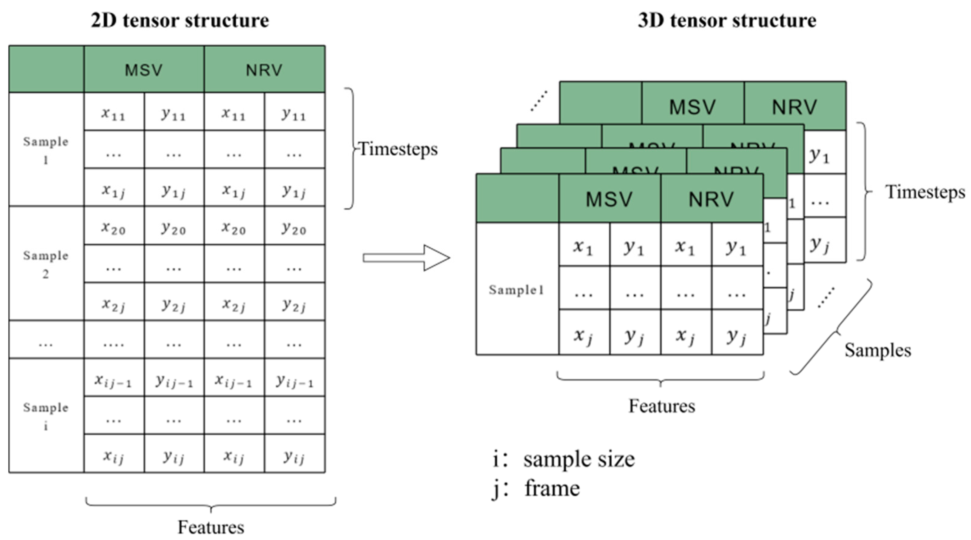
In this study, the initial data consisted of two-dimensional tensors, where each tensor represented a frame of trajectory data for two vehicles involved in a merging scenario. Each frame included the x and y coordinates of both the MSV and the NRV. This structure is suitable for analysis but not directly compatible with the TimeGAN model, which requires a three-dimensional input tensor format.
The three-dimensional tensor format needed by TimeGAN consists of samples, time steps, and features. Each sample represents an individual merging scenario, containing a sequence of frames, and each frame includes the coordinates of the two vehicles.
To convert our two-dimensional data into the required three-dimensional format, we performed a data reconstruction process. This process involved splitting the original files into individual samples: since the data collection frequency was 25 Hz, the total time step of the scenario was composed of key frames, which included 50 frames from the first 2 s and 25 frames from the subsequent 1 s, summing up to 76 frames. Each frame featured four features, which included the coordinates of the two vehicles. As shown in Figure 6, data reorganization of the original 79,116*4 dataset was carried out and converted into three-dimensional tensors (samples, time step, and features) = (1041, 76, and 4).
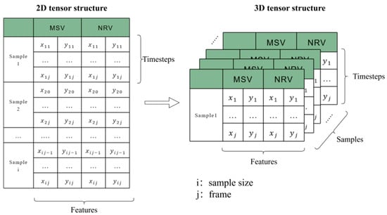
Figure 6.
Data downgrading process.
3.3. TimeGAN
TimeGAN for generating time series data combines the flexibility of the unsupervised GAN framework with the control provided by supervised training in autoregressive models, as proposed by Yoon et al. [39]. Supplementing the unsupervised adversarial loss, a stepwise supervised loss with raw data as supervision was introduced to capture the stepwise conditional distribution in the data. An embedding network provided reversible mapping between features and latent representations, reducing the adversarial learning space’s dimensionality. Joint training of the embedding and generator networks to minimize the supervised loss improved parameter efficiency and enabled the generator to learn temporal relationships.
TimeGAN is composed of four main networks: embedding, recovery, sequence generation, and sequence discrimination. Crucially, its auto-encoding networks (embedding and recovery) are trained together with its adversarial networks (sequence generator and discriminator). This unified training approach enables TimeGAN to encode features, create representations, and process sequences over time. Figure 7a shows the TimeGAN architecture and the roles of each network. The embedding network defines the latent space for the adversarial network’s operation, synchronizing the latent dynamics of both real and synthetic data via supervised loss.
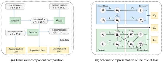
Figure 7.
Structure of TimeGAN (Yoon et al. [39]).
3.3.1. Embedding Functions and Recovery Functions for Self-Encoding Parts
These two functions provided feature space and latent space mappings for the model, used to learn the underlying dynamic relationships of time series data through low-dimensional representations. The embedding function transforms static features and time states into latent space: . The function e is implemented in the recursive function to achieve this transformation, yielding latent encoding representations for static features and time features, denoted as and :
where and represent the embedding networks mapping static features and time features, respectively.
Conversely, the recovery function retrieves feature representations from the latent encoding of static features and temporal features, achieving function r through the feedforward network:
where the recovery networks containing temporal and static characteristics are denoted, respectively, by and . Any architecture can be used to parameterize the two functions, but they must be autoregressive and obey a causal order.
3.3.2. Generators and Discriminators
The TimeGAN model’s generator randomly selects vectors from the vector spaces and of known distributions rather than producing synthetic outputs directly in the feature space, and inputs them into the embedding space, then generates the latent distributions and . Here, and represent the generator networks for generating latent states of static features and latent states of time features , respectively. The generator is implemented through a recursive network that transforms static and temporal random vectors into feature latent encodings and :
The random vectors are sampled from known vector spaces , and is generated stochastically using random sampling. In this model, it is assumed that and follow Gaussian distributions and a Wiener process, respectively.
Similarly, the discriminator processes from the embedding space. The discriminant function takes in the potential encoding of static features and temporal features and returns categories , with representing real states and representing generated states. These are divided into output layer classification functions:
where and represent forward and backward latent state sequences, respectively, while and are the recursive functions. There is no restriction on the structure of the discriminator, and the standard recursive formulation was used in this study.
3.3.3. Joint Learning, Generation, and Iteration
Because of the reversible mapping between the feature space and the latent space, the embedding and recovery functions should accurately reconstruct the latent encoding and of the original data and into the data and . It follows that a reconstruction loss is necessary for the first objective function:
In the TimeGAN model, during adversarial training of the generator and discriminator, the first one receives the original training data and its own previously generated data. Therefore, the second objective function should maximize (for the discriminator) or minimize (for the generator) the likelihood of correctly classifying for and when considering both the training data and as well as the data and that the generator output. Based on the unsupervised loss for computing gradients, the second objective function is:
However, relying solely on the binary adversarial feedback from the discriminator is not sufficient to encourage the generator to capture the stepwise conditional distribution within the data. Therefore, additional losses need to be introduced to further constrain the learning process, with interactive training between cyclic and adversarial. During cyclic training, the generator receives the current state of actual data after being processed by the embedding function and then generates the latent encoding for the next state. The training gradients are computed by capturing the differences between distributions and . The third objective function, the supervised loss function, is calculated using maximum likelihood estimation:
In summary, at each step of training, there is a need to compare the subsequent original latent state from the embedding function with the subsequent latent vector obtained from the generator. Figure 7b illustrates and explains the training mechanism of the three loss functions. The discriminator and the recovery function are trained independently, while the generator and the embedding function are trained jointly.
Here, the loss functions and promote the learning of temporal dynamics and the simulation of real data by the generator, respectively. The parameters of the embedding function as well as the parameters of the recovery function are updated by reconstructing the loss function and the supervised loss function :
where the hyperparameter used to equalize the two losses is λ ≥ 0.
The parameters of the generator network and the parameters of discriminator network are updated from adversarial training:
where another hyperparameter used to equalize the two losses is ≥ 0. The generator minimizes the supervised loss while performing the unsupervised minimum game, allowing TimeGAN to train encoding, generate, and iterate simultaneously. Using , , , and to represent the network parameters for each of the four functions, Figure 8 illustrates the training methodology used by the model and the data transfer process.
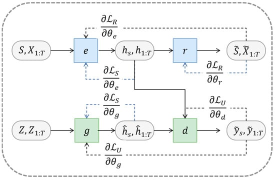
Figure 8.
Network training process (Yoon et al. [39]).
3.4. Evaluation of Generation Quality
Three aspects must be considered in order to assess the quality of generated data: diversity, similarity, and authenticity of the generated samples. The degree to which the distribution of created samples covers the distribution of actual data is referred to as diversity. A common and effective method for evaluating this measure is visualization and dimensionality reduction. In this investigation, principal component analysis (PCA) and t-distributed stochastic neighbor embedding (t-SNE) were employed to scrutinize both the pristine dataset and the synthesized counterpart, whereby temporal information was flattened to project three-dimensional data onto a two-dimensional coordinate plane. This approach facilitated the visual appraisal of the similarity between the distribution of generated samples and that of the original samples.
To validate the similarity between the generated and original trajectories, this study derived the vehicle’s velocity by differentiating the generated continuous coordinate data. By comparing the velocity distributions between the generated and real scenarios, high similarity in the generated samples was inferred if the distributions aligned. The distribution of distances between interacting vehicle pairs was used to further corroborate this result. In addition, the samples generated by a good generative model should be as difficult as possible to be distinguished from the original data by the classification model. If a simple classification model can easily differentiate between generated and real data, this means that the generative model does not perform well. Conversely, if even a sophisticated classification model has difficulty in correctly distinguishing between real and generated data, it indicates a high similarity of the generated data. Therefore, to evaluate the quality of the generated data, a time series classification model using an optimized dual-layer LSTM was trained to differentiate between sequences of original data and generated data. Every created sequence was initially classified as non-real, while every original sequence was labeled as real. Subsequently, to distinguish between the two groups, a ready-made recurrent neural network (RNN) classifier was trained. The similarity was quantitatively assessed through classification error, with the training scores noted as discriminate scores. Using the discriminate score for evaluation, the closer the score is to 0, the more difficult it is for the classification model to distinguish between real and generated data.
Authenticity is used when it is necessary to evaluate whether the generated data can serve practical purposes. In the case of time series data, this means whether the generated data can inherit the predictive characteristics of the original data or, in other words, whether the model can excellently capture the features of time series. Well-generated data should possess predictive capability, meaning they can be used for the prediction of subsequent trajectories. Therefore, a time series prediction model was trained utilizing a RNN with the generated dataset to predict the next time vector for each input sequence. After training, the model was tested on the original dataset. If the prediction results had a good fit with the real data, it indicates that the generated data retained high-quality time series features similar to those of the real data. The mean absolute error (MAE) served as the metric for quantifying the degree of fit and measuring predictive performance. The smaller the error value, the better the prediction effect, indicating that the generated data had good performance in capturing the characteristics of the temporal distribution, and the higher the authenticity. The RNN architecture used for classification and prediction models is illustrated in Figure 9.

Figure 9.
The RNN-based model structure.
3.5. Simulation
The generation of hazardous scenarios was based on naturalistic driving data that can be used for the testing of autonomous vehicles. In order to simplify the experimental model, this study focused only on the feasibility testing of high-risk scenarios generated through the TimeGAN model.
The CARLA simulation platform has been widely used to support development, training, and validation of autonomous driving systems in recent years, favored for its open-source code and open digital assets. CARLA exposes a powerful API that allows users to control all aspects related to the simulation, including traffic generation, pedestrian behaviors, and much more. For this research, the advantages of CARLA include its ability to control a multitude of vehicles with simple autonomous driving capabilities, providing a realistic urban-like environment. Furthermore, CARLA provides a solid foundation for secondary development with its Python (version 3.7) and C++ APIs, which can be flexibly integrated with existing artificial-intelligence-related Python libraries. At the same time, SUMO has a traffic control interface (TraCI), which provides access to all information about the simulation subjects and facilitates cross-platform joint simulation, providing a foundational interface that lays the groundwork for further testing of hazardous scenarios generated in the future. Therefore, the use of co-simulation between CARLA and SUMO can not only use the autonomous vehicle model but also makes it easier to obtain data. The original trajectory data collected from real-world scenarios reflect motion states that conform to vehicular dynamics constraints. However, noise is inevitable in the data generation process, sometimes leading to generated data with significant fluctuations that violate the principles of dynamics. This part of the data requires appropriate processing.
In the data generated from experiments, two types of anomalies were identified. The first and more common anomaly involved vehicle trajectories overlapping or folding back, meaning vehicles appeared to be backing up or turning in place, inconsistent with actual driving behavior. The other type of anomaly was observed as abrupt transitions or shifted too much in some coordinates between two consecutive frames. According to the interval of the original actual speed, we determined a reasonable speed range by exceeding the maximum and minimum values of the actual data by thirty percent. The limit interval for the absolute value of the horizontal velocity was set to be [0, 20], the interval for the vertical velocity was [−10, 12], and the numerical units were both m/s. The data were analyzed with this constraint to identify abnormal data, and the noise was processed to remove these partially fluctuating samples.
Scenario Simulation Test
First, we constructed the roundabout scenario in CARLA in the same manner as the raw data was collected. Maps were retrieved from the OpenStreetMap open-source map collection then imported into RoadRunner. We made sure the roads were meticulously refined on the map to align with the actual roundabout, as the downloaded map could have some missing areas that need to be corrected. Then, we imported the map, which was downloaded from RoadRunner, to CARLA. We set the parameters of each road based on the structural dimensions and speed limits of the real-world roundabout. The CARLA road network was obtained as shown in Figure 10.
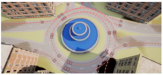
Figure 10.
Roundabout scene in CARLA simulation.
In the traffic scenarios concerning areas where vehicles merge into roundabouts, it is often the responsibility of the drivers in the merging vehicles to make safety judgments to decide when and at what speed to enter the roundabout. In contrast, vehicles circulating within the roundabout typically continue their current path of travel, with drivers rarely needing to consider yielding to merging vehicles. Therefore, during virtual simulation testing, rather than focusing on the functionality of autonomous vehicles driving within the roundabout, it is more crucial to test how autonomous vehicles make decisions when merging into the roundabout.
In the second step, we added two vehicles running within the constructed roundabout environment in CARLA. Vehicle1 was designated as a vehicle circulating within the roundabout, with its vehicle type defined as “CAR”. We used the interface to ensure that the trajectory of V1 followed the trajectory data of the generated nearby roundabout vehicle (NRV). The other vehicle, Vehicle2, represents a vehicle merging into the roundabout. Its vehicle type was defined as “CAV”. The starting position of V2 was specified to ensure it aligned with the starting trajectory data of the generated main subject vehicle (MSV). By setting the endpoint within the internal roads of the roundabout, the objective of V1’s movement was achieved, entering the roundabout and circulating within it. Once the CARLA simulation was up and running, V2 was free to travel, using certain deceleration and avoidance measures when a collision was detected or there was a risk of collision based on the agent from CARLA.
All the generated samples were tested according to the above process, and the trajectories of the “CAV” in the simulated scenario were exported and analyzed together with the trajectories of the “CAR” to determine the danger level of the scenario. The potential encounter time (PET) metric was employed to quantify the severity of conflicts between the merging vehicles and the vehicles circulating within the roundabout.
4. Results and Discussion
4.1. Evaluation of Generated Data
4.1.1. Diversity
In validating the diversity of generated samples, this study employed PCA and t-SNE for dimensionality reduction and visualization, as depicted in Figure 11. The blue dots represent generated samples, while the red dots represent original samples. Since the original scenario is a roundabout, which is a complex scenario with four entrance directions and a large gap between the traffic flows in different directions, the original data suffered from a variety of categories and sample imbalance. This distribution can be clearly found in PCA dimensionality reduction, which is proficient at retaining the global structure of the data. Figure 11a indicates that the overall distribution of generated data was in line with the actual data, but this also implies that PCA’s dimensionality reduction method may not effectively showcase the diversity of the data. On the other hand, t-SNE can preserve the local structure and distance relationships between data samples. As seen in Figure 11b, although the generated data did not completely overlap with the original data, the distribution distance with the original data was close to the original data, indicating good similarity between the two. The distribution range of the generated data demonstrated the existence of diversity among samples. For random events like vehicle interactions, each occurrence varied, and the number of samples that can be collected was limited. Generating samples in this way not only learns the characteristics of the interaction but also generates conflict samples that have not been collected, which provides a new perspective for the establishment of a hazardous scenario library.
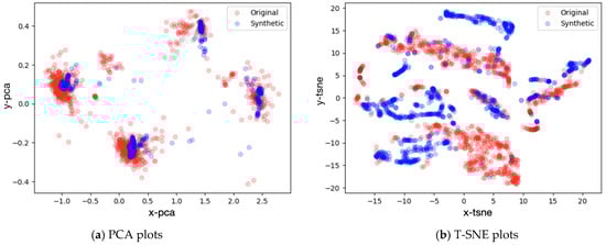
Figure 11.
Visualization results after dimensionality reduction.
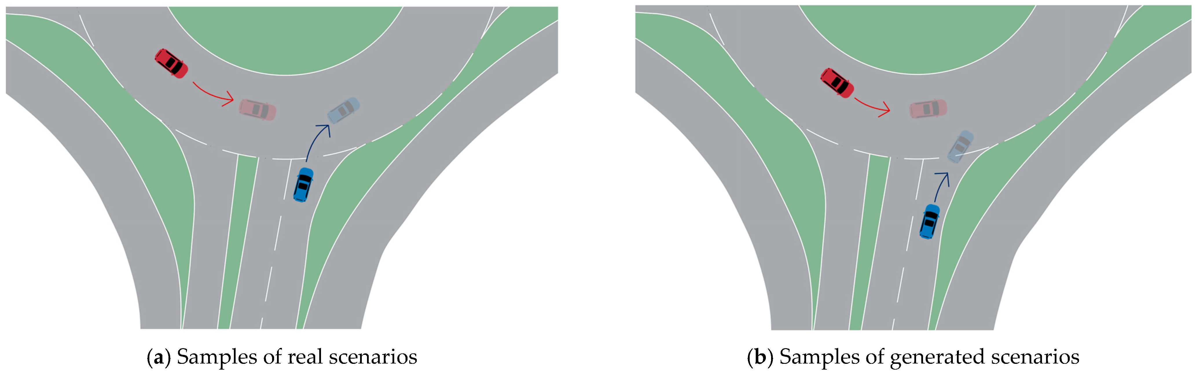
We randomly selected a sample from both the generated and original datasets originating from the same entrance of the scenario. By simply visualizing the trajectories, Figure 12a,b show a generated interaction and the original interaction scenario, respectively. It can be seen that the generated scenario bore a high resemblance to the original one, albeit with its own distinct characteristics. The generated data also conformed to the actual driving pattern and met the dynamic requirements. This indicates that augmenting the dataset through data generation methods can expand the scenario library and enhance diversity.
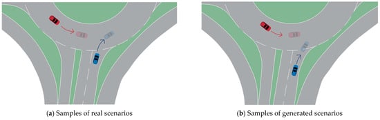
Figure 12.
Scenario visualization.
4.1.2. Similarity and Authenticity
- Kinematic Feature Analysis
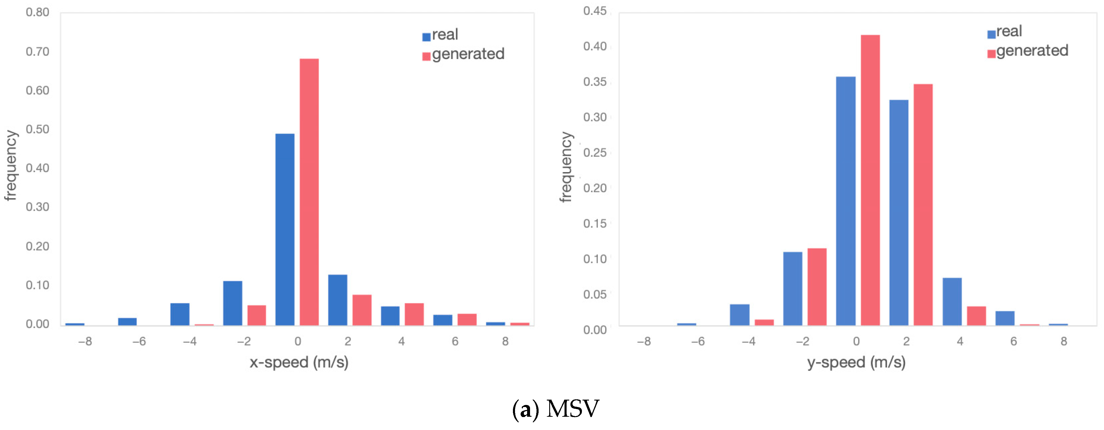
Velocity distributions: Figure 13 depicts the speed distributions of interacting vehicle pairs, both in the horizontal and vertical directions. Figure 13a exhibits the velocity distributions of MSVs in the original and generated scenarios for all samples. Figure 13b exhibits the velocity distributions of NRVs.

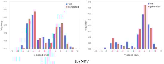
Figure 13.
Comparison of speed distribution between real and generated scenarios.
The TimeGAN model used in this study used coordinate data as the output and input results, so the original and generated data were highly consistent in the distribution of coordinate values. It would be more rigorous to look at the strengths and weaknesses of the generated data even further by calculating the velocities. For the obtained velocity results in the distribution, in the generated scenario both in the horizontal and vertical directions, the distribution pattern was very close to the real ones.
For the MSV, as it is a merging vehicle, it tended to slow down and observe before entering the roundabout, resulting in speeds predominantly concentrated between [−5, 5] m/s. On the other hand, the NRV maintained a steady speed while navigating the roundabout. Although it did not decelerate to yield, its speed during roundabout traversal remained relatively slow, with speeds concentrated in the range [2, 8] m/s regardless of the vehicle’s position. These similarities in the distribution of speeds indicate that the TimeGAN model effectively captured the motion characteristics of both the MSV and NRV. Although there may be slight differences in mathematical features, such as maximum/minimum values, as shown in Table 2, these differences were within expectations and consistent with real-world scenarios.
Table 2.
Comparison between real and generated scenarios.
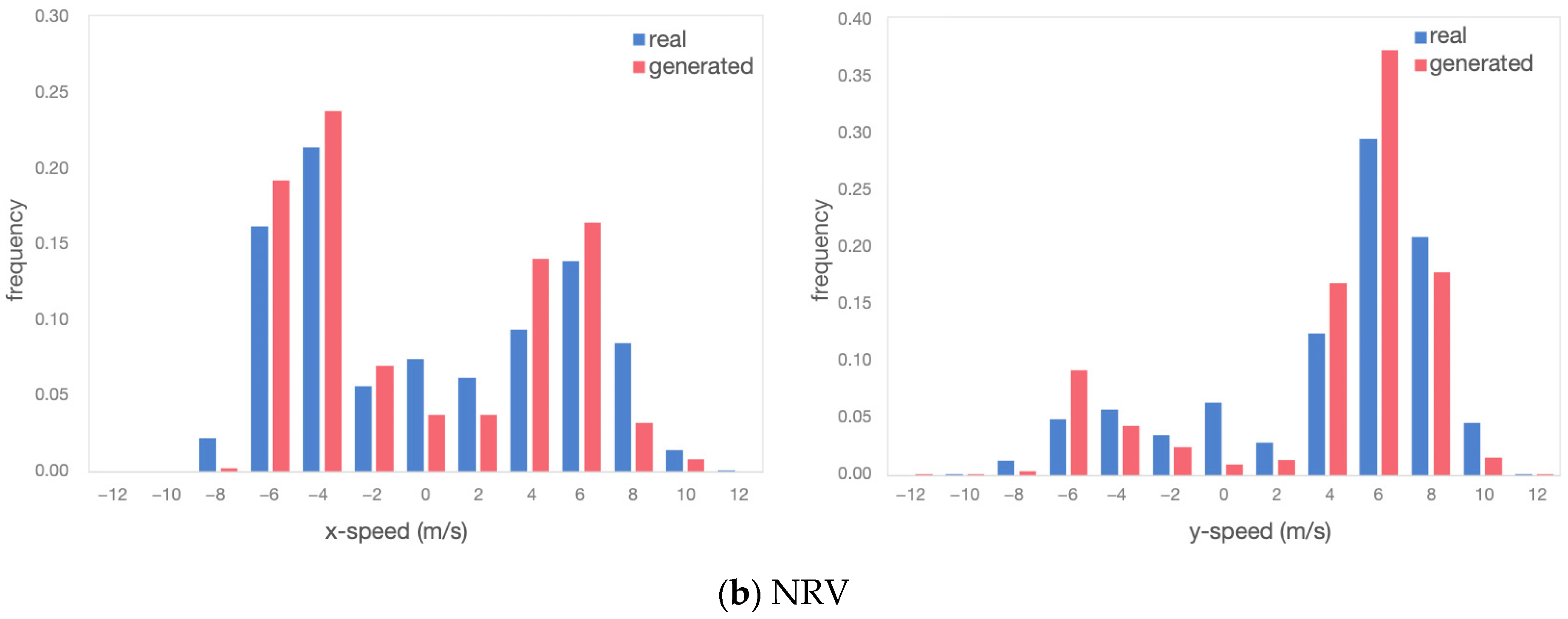
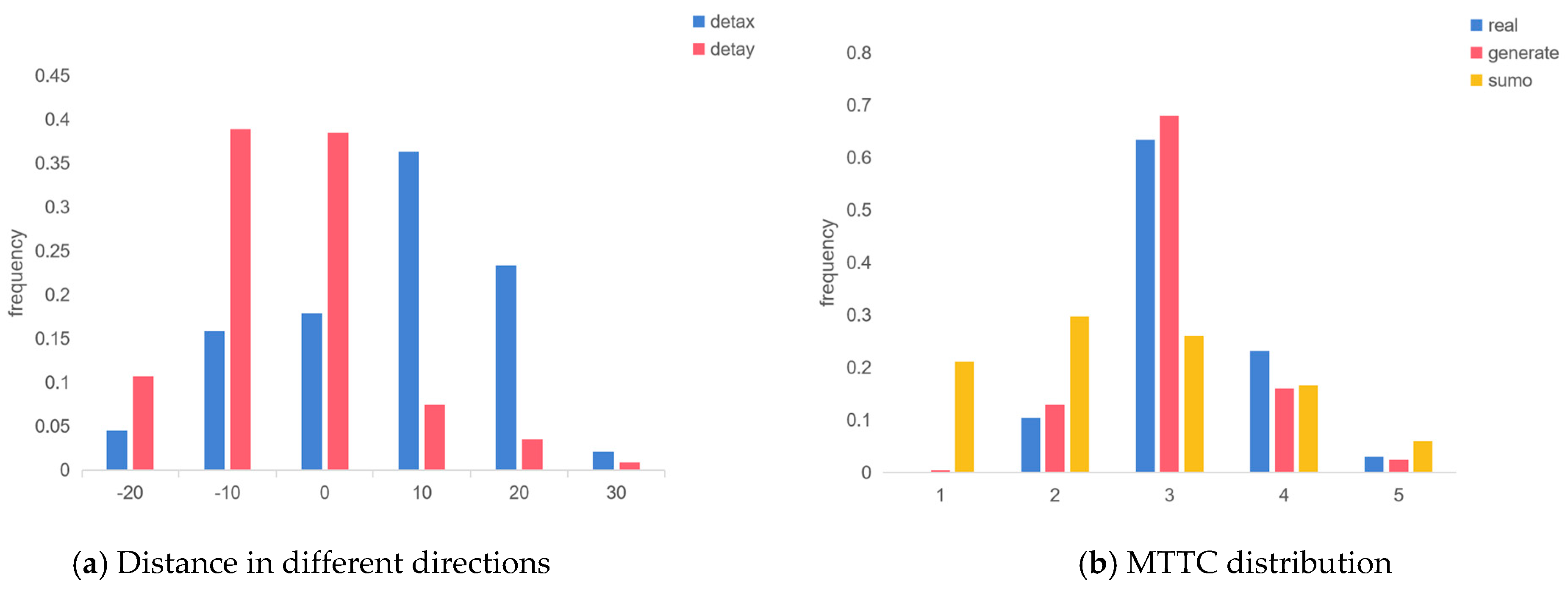
Distance distributions: Figure 14 illustrates the distances between interacting vehicle pairs in the horizontal and vertical directions. The overall distribution patterns of generated and real-world scenario data were consistent. The distances in both directions were mainly concentrated in the range of [−20, 20] m. This consistency was due to the structural characteristics of the roundabout. The horizontal direction of the north–south entrance and the vertical direction of the east–west entrance showed the distance characteristics in the same directions for the interacting vehicles. When paired with the information in Table 2, it was evident that the range of distance distribution was more concentrated in the generated scenario. This trend was also reflected in the distribution of MTTC values, as shown in Figure 15.
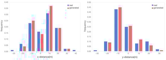
Figure 14.
Comparison of distance distribution between vehicles for real and generated scenarios.
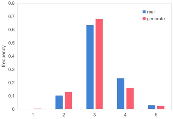
Figure 15.
MTTC distribution.
- 2.
- Hazardous Feature Analysis
Although the MTTC distributions of the generated and real scenarios were very consistent, there were subtle differences. In the generated scenarios, there were more points where the MTTC was less than 3 s, whereas in the real scenarios, there were more points where the MTTC was greater than 3 s. In some extreme cases, the generated scenarios exhibited bolder characteristics. For instance, while real-world scenarios did not feature MTTC values less than 1 s, such instances were observed in generated scenarios.
Overall, the generated trajectory data exhibited a high level of similarity with real trajectory data in terms of distribution and extremum values. However, the generated trajectory data often displayed more hazardous features, such as higher speeds and shorter distances, leading to riskier merging scenarios. This demonstrates that TimeGAN can effectively capture the characteristics of real-world scenarios and is suitable for generating adversarial cases with high risk. It can even generate more dangerous and more valuable adversarial scenarios, which provides a new way to generate dangerous scenarios and is an effective way to expand the library of test scenarios in favor of CAV testing.
- 3.
- Model Evaluation for Similarity and Authenticity
To evaluate the similarity and authenticity of the generated data, two separate models based on recurrent neural networks (RNNs) were developed: one for time series classification and the other for forecasting. The time series classification model discriminated between generated and real data to assess the classification accuracy. The closer the discriminant score of the classification model was to 0, the higher the performance of the classification model, which means that the data generated by the TimeGAN model were of higher quality. A smaller MAE value indicated better prediction performance, which further indicated a higher quality of the data generated by the TimeGAN model. The development of these two models aims to comprehensively assess the similarity and authenticity of the generated data, providing robust evidence for evaluating the performance of the TimeGAN model.
Table 3 presents the results of our experiments. After multiple trials, it could be observed that the optimizer produced better quality data when GRU was chosen and 10,000 iterations were performed. In particular, the optimum achievable result was achieved when the batch size and hidden dim were chosen, and the optimal combination of parameters was 256,180. As indicated in the table, after this round of experiments, the module achieved the optimal discriminative score of 0.0696 and the best predictive score of 0.0488, both of which are very close to 0. These results demonstrate the exceptional performance of our proposed data generation model.
Table 3.
Experimental results for different parameter combinations.
In this section, the quality of the generated scenarios was assessed qualitatively and quantitatively based on aspects such as diversity, similarity, and authenticity. The conclusion drawn is that the scenarios generated by TimeGAN exhibited high quality. Furthermore, they could capture scenarios not encountered in real-world data collection and even depict situations with higher levels of risk than those observed in reality. This provides an effective approach for expanding the testing scenario repository.
4.2. Simulation Result
4.2.1. Simulation Setup and Observations
The generated results were input into CARLA and SUMO for simulation. The NRV followed the generated trajectory during the simulation. However, the actual driving trajectory was slightly different from the generated trajectory, and this difference made the vehicle’s driving state more in line with reality. The MSV only specified its travel task of merging in the roundabout, without limiting the specific travel trajectory.
During the simulation, it was observed that some generated scenarios extended beyond the roadway boundaries, causing vehicles to appear outside the driving area. But such occurrences were relatively rare and predominantly concentrated at specific entry points. Analysis revealed that the sample size of the entrance in the total sample accounted for a very small proportion. This scarcity of samples may have hindered the model’s ability to learn the trajectories of vehicles entering through these specific points. The lack of samples may cause the model not to learn the vehicle trajectory of this entrance well, so that the occurrence of these particular scenarios is understandable. In future research, targeted scenario generation can be performed for these entry points. Out of the 1046 scenarios generated, the scenarios beyond the boundary only accounted for less than 5 percent, which further indicates that it is feasible to use the generative model to generate more vehicle travel scenarios.
4.2.2. Advanced Responses in Simulations
After further simulation of the generated scenarios, it was observed that the MSV, which was not constrained by specific trajectories, tended to exhibit trajectories even more dangerous than those generated originally. Certain conditions occasionally led to triggered collision warnings in SUMO or lateral collisions. Building on this observation within CARLA’s intelligent agent model, the “CAV” would further demonstrate a more advanced response, directly engaging in emergency braking to halt the vehicle, thus averting potential accidents more effectively. After statistical analysis, it was found that 35% of the samples experienced emergency braking scenarios in the CARLA simulation. Furthermore, even when the MSV followed a predefined trajectory and the NRV was controlled by an autonomous driving model, similar situations could still occur. This further illustrates the inherent danger of these generated scenarios. The advanced responses demonstrated by the “CAV” in the CARLA simulation, such as engaging in emergency braking to prevent accidents, underscore the critical nature of these scenarios in real-world driving conditions. To better compare with the original data, simulations were re-run using conventional manually driven vehicle models that do not possess pre-emptive autonomous braking capabilities, and new trajectory information was obtained.
4.2.3. Analysis of Simulation Findings
Figure 16a illustrates the differences in distance between interacting vehicle pairs in both horizontal and vertical directions. It can be observed that these distances were predominantly concentrated within the range of [−10, 10] meters, which is even more concentrated in a closer area than the original and generated scenarios.
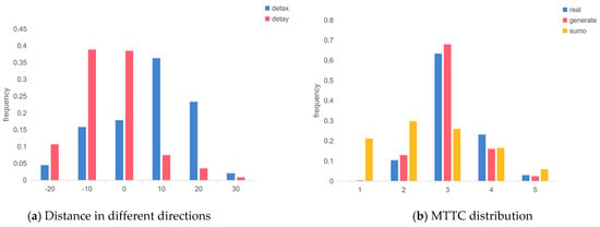
Figure 16.
Simulation results.
The distribution of MTTC values further indicated that most of these simulated scenarios are highly dangerous. As depicted in Figure 16b, instances where the MTTC was less than 2 s were more prevalent. Moments where the MTTC was less than 2 s or even less than 1 s signified situations requiring external intervention to prevent serious collisions. Particularly for the merging part of the roundabout, due to the green cover, the human driver finds it difficult to notice the oncoming traffic from the side, thus leading to aggressive behavior. These special scenarios that require human control or external intervention are exactly the dangerous situations that need to be solved by the self-driving vehicles, and simulation testing with these dangerous scenarios can effectively verify the function of the self-driving vehicles.
5. Conclusions
This study developed a data-driven deep learning framework for generating adversarial hazardous scenarios and devised metrics to evaluate the quality of the generated data. Joint simulation was used to highlight the significance of the generated scenarios. The original data were sourced from the RounD dataset, focusing on vehicle merging scenarios at a genuine roundabout, and extracting hazardous scenarios with adversarial behaviors. The original complex scenario data were culled to leave the trajectory data with critical content, and the dimensions were reduced to horizontal and vertical coordinates at each timeframe. The dynamic information in time series was captured using TimeGAN, which combines adversarial network learning with autoregressive models. The quality of generated lane-changing scenario data was assessed from three critical perspectives: diversity, similarity, and authenticity. Finally, the generated scenarios were tested through the joint simulation using CARLA and SUMO, which confirmed the necessity of generated scenarios in autonomous driving testing. The main conclusions are as follows:
- (a)
- Simplifying scenarios into trajectory data for generation is a rational and effective approach. It allows for the retention of maximum information while enhancing the performance of model training.
- (b)
- For complex scenarios like roundabouts, TimeGAN effectively captured the spatiotemporal features of merging scenarios. It demonstrated the diversity of the generated data, the similarity between the generated and real data, and the feasibility of the generation in various aspects. The analysis validated the effectiveness of this method in expanding the test scenario library.
- (c)
- The developed TimeGAN model effectively generated more high-risk merging scenarios, including adversarial situations not observed in real scenarios. This demonstrates the great potential of generative methods in hazardous scenario testing.
This study still has certain shortcomings. First off, while the TimeGAN model has been investigated for equal-length data, it has not yet been tested for asymmetrical time step sequences. Moreover, it is also necessary to investigate whether the critical scenarios that are important for CAV testing can be further explored in the generated model. The next step to investigate is whether working together with a driving simulator to calibrate cars for different forms of autonomous driving and implement the CAV’s control module functionalities to be tested in the simulation program is feasible.
Author Contributions
Conceptualization, D.R. and Y.L.; methodology, D.R. and J.J.; validation, D.R.; resources, Y.L.; data curation, J.J.; writing—original draft preparation, D.R.; writing—review and editing, Y.L. and J.J.; project administration, H.H. and Y.L.; funding acquisition, H.H. All authors have read and agreed to the published version of the manuscript.
Funding
This research was funded by the National Key Research and Development Program of China, grant number 2023YFB2504704, Changsha Major Science and Technology Projects, grant number kh2401002, the Ministry of Education Foundation for Humanities and Social Sciences, grant number 24YJCZH460, and the Natural Science Foundation of Hunan Province, China, grant number 2024JJ7624.
Institutional Review Board Statement
Not applicable.
Informed Consent Statement
Not applicable.
Data Availability Statement
The original contributions presented in the study are included in the article, further inquiries can be directed to the corresponding author.
Conflicts of Interest
The authors declare no conflicts of interest.
References
- DMV. Autonomous Vehicle Collision Reports. 2024. Available online: https://www.dmv.ca.gov/portal/vehicle-industry-services/autonomous-vehicles/autonomous-vehicle-collision-reports/ (accessed on 27 April 2024).
- Wang, C.; Storms, K.; Winner, H. Online safety assessment of automated vehicles using silent testing. IEEE Trans. Intell. Transp. Syst. 2021, 23, 13069–13083. [Google Scholar] [CrossRef]
- Butz, T.; Paleduhn, S.; Merkel, A.; Bohner, C. Virtual Test of Automated Driving Functions. ATZ Worldw. 2020, 122, 16–21. [Google Scholar] [CrossRef]
- Liu, S.; Ren, F.; Li, P.; Li, Z.; Lv, H.; Liu, Y. Testing Scenario Identification for Automated Vehicles Based on Deep Unsupervised Learning. World Electr. Veh. J. 2023, 14, 208. [Google Scholar] [CrossRef]
- Song, Q.; Tan, K.; Runeson, P.; Persson, S. Critical scenario identification for realistic testing of autonomous driving systems. Softw. Qual. J. 2023, 31, 441–469. [Google Scholar] [CrossRef]
- Althoff, M.; Lutz, S. Automatic generation of safety-critical test scenarios for collision avoidance of road vehicles. In Proceedings of the 2018 IEEE Intelligent Vehicles Symposium (IV), Changshu, China, 26–30 June 2018; pp. 1326–1333. [Google Scholar]
- Donzé, A. Breach, a toolbox for verification and parameter synthesis of hybrid systems. In Proceedings of the 22nd International Conference on Computer Aided Verification, CAV 2010, Proceedings 22, Edinburgh, UK, 15–19 July 2010; Springer: Berlin/Heidelberg, Germany, 2010; pp. 167–170. [Google Scholar]
- Tuncali, C.E.; Pavlic, T.P.; Fainekos, G. Utilizing S-TaLiRo as an automatic test generation framework for autonomous vehicles. In Proceedings of the 2016 IEEE 19th International Conference on Intelligent Transportation Systems (ITSC), Rio de Janeiro, Brazil, 1–4 November 2016; pp. 1470–1475. [Google Scholar]
- Karunakaran, D.; Worrall, S.; Nebot, E. Efficient statistical validation with edge cases to evaluate highly automated vehicles. In Proceedings of the 2020 IEEE 23rd International Conference on Intelligent Transportation Systems (ITSC), Rhodes, Greece, 20–23 September 2020; pp. 1–8. [Google Scholar]
- Koren, M.; Alsaif, S.; Lee, R.; Kochenderfer, M.J. Adaptive stress testing for autonomous vehicles. In Proceedings of the 2018 IEEE Intelligent Vehicles Symposium (IV), Changshu, China, 26–30 June 2018; pp. 1–7. [Google Scholar]
- Lee, R.; Kochenderfer, M.J.; Mengshoel, O.J.; Brat, G.P.; Owen, M.P. Adaptive stress testing of airborne collision avoidance systems. In Proceedings of the 2015 IEEE/AIAA 34th Digital Avionics Systems Conference (DASC), Prague, Czech Republic, 13–17 September 2015; pp. 6C2-1–6C2-13. [Google Scholar]
- Feng, S.; Yan, X.; Sun, H.; Feng, Y.; Liu, H.X. Intelligent driving intelligence test for autonomous vehicles with naturalistic and adversarial environment. Nat. Commun. 2021, 12, 748. [Google Scholar] [CrossRef] [PubMed]
- Xu, Y.; Zou, Y.; Sun, J. Accelerated testing for automated vehicles safety evaluation in cut-in scenarios based on importance sampling, genetic algorithm and simulation applications. J. Intell. Connect. Veh. 2018, 1, 28–38. [Google Scholar] [CrossRef]
- Zhang, S.; Peng, H.; Zhao, D.; Tseng, H.E. Accelerated evaluation of autonomous vehicles in the lane change scenario based on subset simulation technique. In Proceedings of the 2018 21st International Conference on Intelligent Transportation Systems (ITSC), Maui, HI, USA, 4–7 November 2018; pp. 3935–3940. [Google Scholar]
- Christian, K.; Frank, D. Data-driven test scenario generation for cooperative maneuver planning on highways. Appl. Sci. 2020, 10, 8154. [Google Scholar] [CrossRef]
- Jenkins, I.R.; Gee, L.O.; Knauss, A.; Yin, H.; Schroeder, J. Accident scenario generation with recurrent neural networks. In Proceedings of the 2018 21st International Conference on Intelligent Transportation Systems (ITSC), Maui, HI, USA, 4–7 November 2018; pp. 3340–3345. [Google Scholar]
- Jin, J.; Huang, H.; Yuan, C.; Li, Y.; Zou, G.; Xue, H. Real-time crash risk prediction in freeway tunnels considering features interaction and unobserved heterogeneity: A two-stage deep learning modeling framework. Anal. Methods Accid. Res. 2023, 40, 100306. [Google Scholar] [CrossRef]
- Ding, W.; Xu, C.; Arief, M.; Lin, H.; Li, B.; Zhao, D. A survey on safety-critical driving scenario generation—A methodological perspective. IEEE Trans. Intell. Transp. Syst. 2023, 24, 6971–6988. [Google Scholar] [CrossRef]
- Ding, W.; Xu, M.; Zhao, D. Cmts: A conditional multiple trajectory synthesizer for generating safety-critical driving scenarios. In Proceedings of the 2020 IEEE International Conference on Robotics and Automation (ICRA), Paris, France, 31 May–31 August 2020; pp. 4314–4321. [Google Scholar]
- Małecki, K.; Wątróbski, J.; Wolski, W. A cellular automaton based system for traffic analyses on the roundabout. In Computational Collective Intelligence: 9th International Conference, ICCCI 2017, Nicosia, Cyprus, September 27-29, 2017, Proceedings, Part II 9; Springer International Publishing: Cham, Switzerland, 2017; pp. 56–65. [Google Scholar]
- Mamlouk, M.; Souliman, B. Effect of traffic roundabouts on accident rate and severity in Arizona. J. Transp. Saf. Secur. 2019, 11, 430–442. [Google Scholar] [CrossRef]
- Al-Ghandour, M.N.; Schroeder, B.J.; Williams, B.M.; Rasdorf, W.J. Conflict Models for Single-Lane Roundabout Slip Lanes from Microsimulation: Development and Validation. Transp. Res. Rec. J. Transp. Res. Board 2011, 2236, 92–101. [Google Scholar] [CrossRef]
- Guo, R.J. A Study on the Capacity of Circular Intersections Based on Gap Acceptance Theory. Doctoral Dissertation, Beijing Jiaotong University, Beijing, China, 2013. [Google Scholar]
- Nafis, A.; Mohamed, A.; Amrita, G.; Ou, Z. Investigating surrogate safety measures at midblock pedestrian crossings using multivariate models with roadside camera data. Accid. Anal. Prev. 2023, 192, 107233. [Google Scholar]
- Kumar, A.; Paul, M.; Ghosh, I. Analysis of Pedestrian Conflict with Right-Turning Vehicles at Signalized Intersections in India. J. Transp. Eng. Part A Syst. 2019, 145, 04019018. [Google Scholar] [CrossRef]
- Xin, F.; Wang, X.; Sun, C. Risk evaluation for conflicts between crossing pedestrians and right-turning vehicles at intersections. Transp. Res. Rec. J. Transp. Res. Board 2021, 2675, 1005–1014. [Google Scholar] [CrossRef]
- Ozbay, K.; Yang, H.; Bartin, B.; Mudigonda, S. Derivation and Validation of New Simulation-Based Surrogate Safety Measure. Transp. Res. Rec. J. Transp. Res. Board 2008, 2083, 105–113. [Google Scholar] [CrossRef]
- Charly, A.; Mathew, T.V. Estimation of traffic conflicts using precise lateral position and width of vehicles for safety assessment. Accid. Anal. Prev. 2019, 132, 105264. [Google Scholar] [CrossRef] [PubMed]
- Mirza, M.; Osindero, S. Conditional generative adversarial nets. arXiv 2014, arXiv:1411.1784. [Google Scholar]
- Krajewski, R.; Moers, T.; Meister, A.; Eckstein, L. Béziervae: Improved trajectory modeling using variational autoencoders for the safety validation of highly automated vehicles. In Proceedings of the 2019 IEEE Intelligent Transportation Systems Conference (ITSC), Auckland, New Zealand, 27–30 October 2019; pp. 3788–3795. [Google Scholar]
- Krajewski, R.; Moers, T.; Nerger, D.; Eckstein, L. Data-driven maneuver modeling using generative adversarial networks and variational autoencoders for safety validation of highly automated vehicles. In Proceedings of the 2018 21st International Conference on Intelligent Transportation Systems (ITSC), Maui, HI, USA, 4–7 November 2018; pp. 2383–2390. [Google Scholar]
- Sumiya, Y.; Horie, K.; Shiokawa, H.; Kitagawa, H. Nr-gan: Noise reduction gan for mice electroencephalogram signals. In ICBSP ‘19, Proceedings of the 2019 4th International Conference on Biomedical Imaging, Signal Processing, Nagoya, Japan, 17–19 October 2019; Association for Computing Machinery: New York, NY, USA, 2020; pp. 94–101. [Google Scholar]
- Wiese, M.; Knobloch, R.; Korn, R.; Kretschmer, P. Quant GANs: Deep generation of financial time series. Quant. Financ. 2020, 20, 1419–1440. [Google Scholar] [CrossRef]
- Cao, C.; Li, M. Generating mobility trajectories with retained data utility. In KDD ‘21, Proceedings of the 27th ACM SIGKDD Conference on Knowledge Discovery & Data Mining, Virtual Event Singapore, 14–18 August 2021; Association for Computing Machinery: New York, NY, USA, 2021; pp. 2610–2620. [Google Scholar]
- Yang, B.; Yan, G.; Wang, P.; Chan, C.-Y.; Song, X.; Chen, Y. A novel graph-based trajectory predictor with pseudo-oracle. IEEE Trans. Neural Netw. Learn. Syst. 2021, 33, 7064–7078. [Google Scholar] [CrossRef] [PubMed]
- Tang, C.; Salakhutdinov, R.R. Multiple futures prediction. In Proceedings of the 33rd International Conference on Neural Information Processing Systems, Vancouver, BC, Canada, 8–14 December 2019; Volume 32. [Google Scholar]
- Andreas, D.; Henrik, A.; Sadegh, R.; Morteza, H.C. A deep learning framework for generation and analysis of driving scenario trajectories. SN Comput. Sci. 2023, 4, 251. [Google Scholar]
- Arnelid, H.; Zec, E.L.; Mohammadiha, N. Recurrent conditional generative adversarial networks for autonomous driving sensor modelling. In Proceedings of the 2019 IEEE Intelligent transportation systems conference (ITSC), Auckland, New Zealand, 27–30 October 2019; pp. 1613–1618. [Google Scholar]
- Yoon, J.; Jarrett, D.; Van der Schaar, M. Time-series generative adversarial networks. In Proceedings of the 33rd International Conference on Neural Information Processing Systems, Vancouver, BC, Canada, 8–14 December 2019; Volume 32. [Google Scholar]
- Krajewski, R.; Moers, T.; Bock, J.; Vater, L.; Eckstein, L. The round dataset: A drone dataset of road user trajectories at roundabouts in germany. In Proceedings of the 2020 IEEE 23rd International Conference on Intelligent Transportation Systems (ITSC), Rhodes, Greece, 20–23 September 2020; pp. 1–6. [Google Scholar]


Disclaimer/Publisher’s Note: The statements, opinions and data contained in all publications are solely those of the individual author(s) and contributor(s) and not of MDPI and/or the editor(s). MDPI and/or the editor(s) disclaim responsibility for any injury to people or property resulting from any ideas, methods, instructions or products referred to in the content. |
© 2025 by the authors. Licensee MDPI, Basel, Switzerland. This article is an open access article distributed under the terms and conditions of the Creative Commons Attribution (CC BY) license (https://creativecommons.org/licenses/by/4.0/).