Abstract
This study optimized the constants of the RNG k-ε model using the Ensemble Kalman Filter (ENKF) data assimilation method to improve the accuracy of air-lift plunger gap flow predictions. For high Reynolds number turbulent flow, we conducted numerical simulations integrating experimental data with a library of predicted data generated via optimal Latin hypercube sampling. ENKF was employed to assimilate these data and adjust the model constants, significantly reducing prediction errors and enhancing the accuracy of plunger models. Specifically, mean square errors for rectangular and circular plungers decreased from 60.67 and 61.48 to 7.12 and 7.20, respectively. The study also revealed significant changes in vortex dynamics and flow distribution following data assimilation, providing insights for optimizing plunger design and improving system energy efficiency. These findings underscore the potential of data assimilation in advancing oil and gas production.
1. Introduction
In the middle and late stages of a natural gas field’s development, the reduction in formation pressure often renders the gas incapable of autonomously removing the accumulated formation water. This frequently results in a decline in the production capacity of the gas wells, potentially leading to their abandonment [1]. Therefore, to effectively address this issue, plunger lift technology has been widely adopted as a cost-effective artificial lift method [2]. This technique involves deploying a plunger in the wellbore to facilitate efficient gas-liquid separation and liquid discharge [3].
Current research on gas-lift plunger performance primarily employs experimental measurements and numerical simulations, both of which have inherent limitations. Experimentally, the process involves high costs and complex equipment setup, often requiring on-site trials. Experiments are constrained by actual gas well conditions, making it difficult to replicate various operating conditions, thereby limiting the general applicability of the results. Additionally, experiments are time-consuming, especially when repeated under different conditions. Due to environmental influences on measurement, experimental results often contain significant errors. Particularly in gas-lift plunger experiments, the small gap between the plunger and the pipeline makes it challenging to measure physical quantities within the gap, which are crucial for characterizing the plunger’s flow field.
For numerical simulations, the reliance is on established models and assumptions, which may not fully reflect real-world scenarios. The flow field around a gas-lift plunger, characterized by high velocities, large gradients, small gaps, and curved streamlines, complicates the flow, necessitating the use of appropriate turbulence models to accurately describe turbulence structures and their impacts. The Reynolds-averaged Navier-Stokes (RANS) method, blending theory and empiricism, is a viable simulation technique. However, its turbulence model accuracy relies on specific model constants, usually calibrated with standard flows like flat plate boundary layers and free shear flows, which may be inadequate for predicting complex flow fields in gas-lift plungers [4].
Traditional computational fluid dynamics (CFD) techniques, such as Direct Numerical Simulation (DNS) and Large Eddy Simulation (LES), can effectively model gas flow. However, their requirement to handle high Reynolds number turbulence necessitates substantial computational resources, which in turn limits their practical engineering applications [5]. Currently, the Reynolds-averaged Navier-Stokes (RANS) equations remain the mainstream choice for engineering applications due to their favorable balance between computational cost and predictive accuracy.
Given these limitations, there is a clear need to develop more accurate and efficient modeling techniques for gas-lift plunger systems. Accurate modeling not only enhances the fundamental understanding of near-wall turbulence and flow resistance within narrow annular gaps but also enables the optimization of plunger geometry and operating parameters through numerical tools. Furthermore, improved modeling fidelity provides a basis for digital twin technologies and intelligent well management systems.
In geosciences, data assimilation (DA) has been developed as a technique to address potential shortcomings in experimental and numerical simulations, establishing it as a fourth central analytical approach alongside theoretical, experimental, and numerical methods [6]. DA is a method that integrates mathematical models with observational data, considering the uncertainties of both. It combines measured data with predictive models to adjust the model’s evolution, optimize performance, and enhance accuracy. Data assimilation was initially proposed by Lewis Fry Richardson to optimize weather forecasting [7]. Subsequently, this approach has been applied to system monitoring, hydrology, and geology, among other fields [8].
This technique pioneers a novel approach to turbulence research, facilitating more precise simulations and predictions of turbulence behavior and offering more reliable guidance for engineering applications. Kato et al. [9] developed a data assimilation method based on the ensemble transformed Kalman filter (ETKF) and successfully predicted the inlet angle of attack and the Mach number for the turbulent flow field around an airfoil. Deng et al. [10] optimized the constants in four turbulence models using an EnKF-based DA technique. Analyzing Particle Image Velocimetry data from a free circular jet flow showed significant improvements in flow field predictions across all models after optimization, with the k-ε model exhibiting the best performance. Zhang et al. [11] conducted an in-depth study on the applicability of the hybrid data assimilation method (EnVar) in turbulence modeling. From the perspective of Bayesian inference, the research optimized RANS simulations for a converging-diverging channel. Experimental results demonstrated that the ensemble-based variational method effectively inferred unknown parameters under both small-sample conditions (D = 20) and large-scale systems (D = 2400). He et al. [12] employed a data assimilation approach, utilizing the Ensemble Kalman Filter (EnKF) combined with NASA’s PIV experimental data to optimize the constants of the Spalart-Allmaras (SA) turbulence model. The optimized model improved the accuracy of jet flow field predictions, reducing the relative error in the horizontal direction behind the nozzle from 13.04% to 4.6%. Fang et al. [13] used the Ensemble Kalman Filter (EnKF) algorithm to recalibrate the constants of the SST k-ω turbulence model, significantly improving the accuracy of flow characteristic predictions for steam valves with filters. The recalibrated model constants are suitable for conditions with similar valve openings but exhibit higher errors when the opening differences are large. The optimized model constants better capture the turbulence characteristics of the internal flow. Liu et al. [14] developed a data-driven framework using a two-step EnKF method to predict compressor cascade flow fields. Validating with a test function, they applied S-A and SST models to the MAN GHH cascade, achieving predictions consistent with experiments. Data assimilation reduced errors by nearly 70%, improved separation bubble predictions, and showed low dependency on turbulence models. Yu et al. [15] utilized the EnKF DA technique to optimize the SST k-ω turbulence model constants for enhancing heat transfer predictions in plate heat exchangers. By assimilating experimental data from various operational conditions into the computational model, the study achieved significant reductions in prediction errors. The calibrated model constants enabled more accurate simulations of the complex flow and heat transfer behaviors within plate heat exchangers. This optimization, validated by experimental data, substantially enhanced the accuracy of flow predictions, offering a more precise method for analyzing the flow characteristics of the control valve. Meng et al. [16] optimized S-A turbulence model parameters using the Ensemble Kalman Filter (EnKF) for three wind turbine airfoils (NACA63415, S809, DU97W300) under stall conditions. The optimized parameters reduced simulation errors, improved flow separation predictions, and showed that S809’s parameters could be applied to other airfoils with slightly higher errors. Key parameters Cb1, Cu1, and σ changed significantly, with Cb1 being the most critical.
Despite extensive research in related fields, studies on data assimilation for air-lift plungers remain scarce, particularly regarding the scalability of assimilated models. This paper employs the Ensemble Kalman Filter (EnKF) algorithm to recalibrate turbulence model constants through data assimilation techniques. By integrating experimental data with numerical simulations, the study evaluates the scalability of various plungers under different operational conditions. A comparative analysis is conducted to examine the flow characteristics and states of the gas-lifted plunger gap flow before and after model optimization. It is crucial to emphasize that the assimilation process requires high-fidelity experimental data. In this study, gas is used as the sole flow medium, with the flow rate during plunger hovering serving as the observational data. This approach aims to investigate the gas flow characteristics as it passes through the plunger gap, ultimately providing a more accurate and practical theoretical foundation for enhancing plunger lifting techniques.
Furthermore, the findings of this study are expected to contribute to the broader field of turbulent flow modeling by extending data assimilation techniques to gas–liquid two-phase systems, while also offering technical insights that may enhance the efficiency, reliability, and design optimization of plunger lift operations in low-pressure gas wells.
2. Mathematical Principles
2.1. Turbulence Modeling Equations
Due to the irregular rod-like external structure of the plunger, the fluid dynamics around it become highly complex. This complexity stems not only from the plunger’s geometry but also from the fluid flow behavior both around and within the plunger. To effectively simulate and analyze this intricate flow scenario, the RNG k-ε model, an enhanced version of the standard k-ε model, provides an ideal solution. By incorporating additional correction terms, this model can accurately handle strong vortex flows and flow distortions around curved surfaces, thereby improving the precision of turbulence simulations. The RNG k-ε model excels in simulating flow fields both inside and outside the plunger, effectively capturing subtle flow variations and vortex structures [17].
RNG k-ε model equations:
k equation:
ε equations:
In these equations, Gk represents the turbulent kinetic energy produced by the mean velocity gradient
is the turbulent kinetic energy generated by buoyancy.
represents the contribution of pulsating expansion to the total dissipation rate in compressible turbulence.
represents the source term defined by the use.
The reciprocal of the effective Prandtl number, , is analytically determined using RNG theory, with .
In Fluent, the default constants of the RNG k-ε turbulence model are modifiable, including: .
2.2. Ensemble Kalman Filter
The Ensemble Kalman Filter (EnKF) is a DA method designed for state estimation in nonlinear systems. This method was proposed by Evensen et al. [18] to address the limitations of the traditional Kalman Filter (KF) when applied to nonlinear systems. The EnKF uses an ensemble of samples to represent the probability distribution of the system’s state and adjusts the samples to more closely align with experimental observations by calculating their covariance matrix and the Kalman gain [19].
The subject of study is represented by a set of state variables, denoted collectively as the vector . Experimental observations are represented as the vector . The algorithm assumes a specific relationship exists among state variables, experimental observations, and predictive models.
The state-space model describing the relationship between the experimental observations and prediction model is:
In the formula:
: prediction model function.
: initial state vector of the samples.
: prediction model error (neglected in this study).
: observation matrix mapping the state vector to observation space.
: experimental observation error.
- (1)
- Forecasting process
During the prediction process, the state parameter vector within each ensemble member will be iteratively computed using the RNG k-ε model starting from the initial state until the numerical simulation of turbulence converges.
The updating of the state parameters follows the following equation:
Here, F represents the governing equations of the RNG k-ε turbulence model, and the state parameters of each ensemble member are expressed in the following form:
Here, Q denotes the gas volumetric flow rate predicted by the RNG k-ε model, and A is the vector of turbulence model constants, expressed as: A = (Cu C1ε C2ε Prt)T. The superscript i denotes the index of the ensemble member.
Mean value of the ensemble members:
where represents the total number of set members, and denotes the average value of the set members.
- (2)
- Analysis process
The analysis phase is a critical step in the ENKF algorithm. In this phase, the Kalman gain is determined, and the ensemble members are updated by synthesizing the uncertainty of observational data with the statistical information of the ensemble members. The specific process is as follows:
Prediction error analysis:
Here,
Kalman gain calculation:
Updating collection members:
Mean value of the corresponding new set member:
For highly nonlinear models, a relatively accurate prediction is often not achieved by performing the analysis process only once. Consequently, this study employs a multi-iteration EnKF algorithm for both prediction and analysis. By iterating multiple times, the uncertainty of observational data and the statistical properties of the ensemble members can be more comprehensively incorporated, thereby enhancing the precision of predictions. At each iteration, the convergence of the algorithm is assessed based on the standard deviation of the ensemble members and the maximum number of iterations, which is set to 10,000. Utilizing this multi-iteration EnKF algorithm enables a more accurate approximation of the system’s actual state, improves prediction accuracy, and ensures algorithmic convergence.
2.3. Model Calibration Process
This paper uses the EnKF in the data assimilation method to calibrate the model’s constants. In this method, we define an ensemble state matrix of the following form:
Here, k denotes the number of state variables, which is 5 in this study.
The experimental flow rate observation data are as follows:
represents the experimentally measured gas volumetric flow rate under specific conditions.
The observation matrix for data assimilation is as follows:
where W is the observation error derived from the uncertainty of the measurement instruments.
The mapping function matrix is as follows:
Here, 1m×n denotes an m × n matrix with all elements equal to 1, In represents the identity matrix of order n, and 0m×n indicates an m × n matrix with all elements equal to 0.
In this study, the observation matrix H is employed to extract the predicted gas volumetric flow rate Q from the state vector and project it onto the observation space, corresponding to the experimentally measured volumetric flow rate. The observation matrix is explicitly defined as follows:
This indicates that only the first variable of the state vector (the gas volumetric flow rate) is directly compared with the experimental observations.
In this study, 100 samples, corresponding to the total number of ensemble members (L = 100), are generated through Latin hypercube sampling and selected for calibrating the turbulence model constants. The predicted flow rates for these 100 samples under specific operating conditions are obtained using RNG k-ε model calculations. According to the integration method in Equation (17), these 100 sets of predicted flow rates serve as the initial state matrix for the algorithm. Subsequently, the initial state matrix is updated through several iterations of the ensemble Kalman filtering algorithm, using experimentally observed flow data to derive the optimal model constants calibrated through data assimilation. Finally, the newly calibrated model constants are applied under various operating conditions to evaluate their reliability and applicability. The entire process is illustrated in Figure 1.
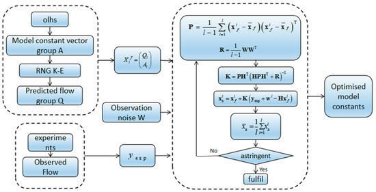
Figure 1.
Model constant calibration procedure based on experiment data assimilation.
3. Experimental Procedure and Equipment
In the study of gas-lift plunger flow fields, conventional flow measurement techniques are difficult to apply due to the extremely narrow clearance between the plunger and the tubing wall (typically on the millimeter scale) and the confined, compact structure. Although hot-wire/hot-film anemometry (HWA/HFA) [20] offers fast response, the probe is relatively large and tends to disturb the flow. Particle Image Velocimetry (PIV) and Particle Tracking Velocimetry (PTV) require transparent test sections and laser illumination, and the tracer particles are significantly affected by wall adhesion effects and plunger motion. Laser Doppler Velocimetry (LDV), while highly accurate, can only provide point measurements and also relies on optical access, making it difficult to capture the overall flow structure within the narrow, complex clearance [21].
Therefore, in this study, the flow rate observed when the gas-lift plunger is suspended in the well is used as the measurement input, and the flow characteristics are then inferred through data assimilation.
3.1. Calibration of Turbulence Modeling Constants
The experimental apparatus consists of core components, an auxiliary system, and an observation system, primarily constructed from plexiglass and high-strength stainless steel.
The core components include a steel frame, tubing frame assembly, tubing components, and plungers with various slot geometries. The entire structure is built on a 7-m-high steel framework, with its top securely anchored to the ceiling and wall to mitigate structural vibrations, while the base is firmly fixed to the ground using four sets of anchor bolts. The tubing frame assembly comprises a blowout preventer, a well-bottom buffering device, and a plexiglass tubing section with an inner diameter of 60 mm and a wellbore length of 6 m.
The auxiliary system consists of an air compressor, a gas storage tank, and adjustable control valves. The observation system includes a gas flow meter positioned at the gas inlet and pressure transmitters installed at the gas inlet, well bottom, and wellhead.
The primary equipment parameters are presented in Table 1, while the experimental setup for evaluating the sealing performance of the gas-lift plunger is illustrated in Figure 2.

Table 1.
Main equipment parameters.
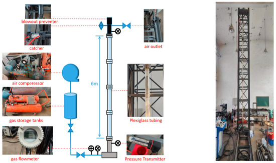
Figure 2.
Plunger lifting simulation experiment device diagram.
According to the optimal diameter ratio proposed by Zhao et al. [22], the outer diameter of the plunger was set to 57.6 mm. Based on the findings of Wang et al. [23], the rectangular slot, which exhibits the poorest sealing performance, and the arc-shaped slot, which demonstrates the best sealing performance, were selected as the sealing slot structures for the plunger’s exterior. The rectangular slot has a depth of 6 mm and a width of 12 mm, while the arc-shaped slot has a radius of 6 mm and is designed as a complete semicircle. The experimental plunger device, as illustrated in Figure 3, is constructed from stainless steel, with each plunger weighing 3.5 kg.
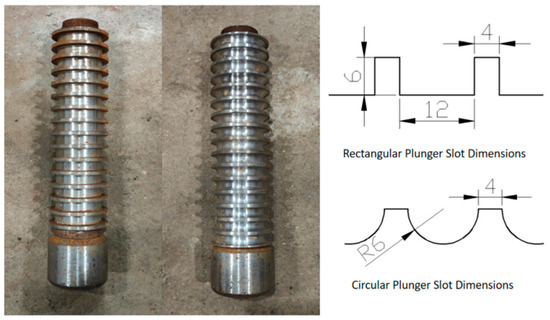
Figure 3.
Plunger device for the experiment.
3.2. Experimental Method
The objective of the experiment is to obtain the volumetric flow rate of gas when the plunger is in a suspended state at various positions within the wellbore, as well as the corresponding pressure readings at the flow meter, well bottom, and wellhead. The working fluid used in the experiment is air, with a temperature of 15 °C and operated under standard atmospheric pressure.
The sealing performance of the air-lifted plunger was evaluated as follows:
- After verifying and confirming the integrity of the experimental apparatus, the required test plunger structure is installed. The plunger is introduced into the system through the top of the device, and the air compressor is activated to store compressed air, providing the necessary gas supply for the experiment.
- A cushioning plug is installed at the top of the tubing to ensure the stability and safety of the plunger during the testing process and to prevent potential accidents.
- The intake valve is opened, and the gas flow rate is gradually increased until the plunger begins to exhibit signs of activation. By precisely controlling the gas flow, the plunger is brought to a state of upward motion. The flow rate is then finely adjusted so that the plunger reaches and maintains a stable hovering position, as illustrated in Figure 4. Once in position, the plunger is held in suspension for 10 s, during which the inlet flow rate, inlet pressure, bottom-hole pressure, and wellhead pressure are recorded. Data are collected at a sampling frequency of one measurement per second, and the average values during this steady-state period are subsequently calculated.
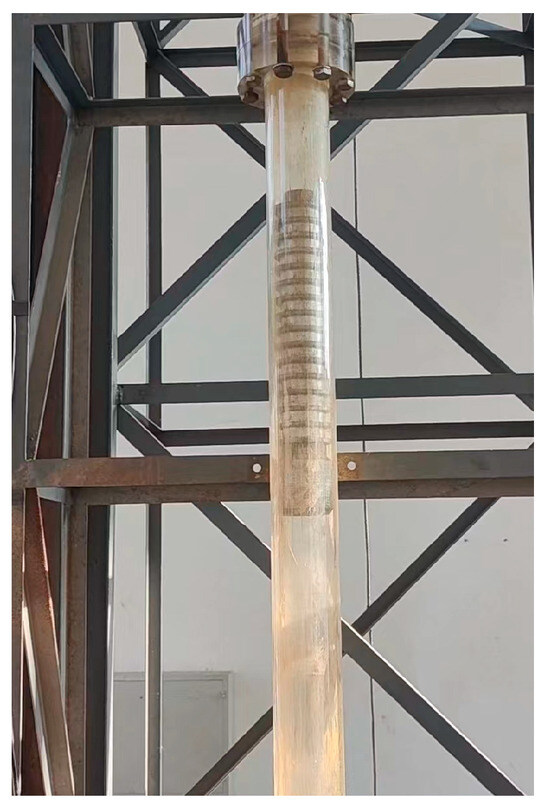 Figure 4. Plunger hovering state.
 - Based on the experimental data, the gas flow rate is corrected using the ideal gas law to calculate the volumetric flow rate under standard conditions (0 °C, 101.325 kPa):
: Gas volumetric flow rate under standard conditions (m3/h);
: Measured gas flow rate (m3/h);
: Measured absolute gas pressure (Pa);
: Standard atmospheric pressure (101,325 Pa);
: Measured absolute gas temperature (K);
: Standard temperature (273.15 K)
Adjust the opening of the outlet valve to control the hovering position of the plunger, and repeat step (3) multiple times.
- 5.
- Replace the plunger and repeat steps 1–4.
3.3. Experimental Results
The measured experimental data are displayed in Table 2, where one set is utilized for experimental data assimilation to optimize the turbulence model constants, and the remainder is used for validation.
Table 2.
Experimental test results.
4. Examples of Numerical Simulation Calculations
The geometric model and computational grid of the plunger lift model are shown in Figure 4. The dimensions of the plunger and tubing are based on the experimental setup. The distance from the inlet to the plunger is 70 mm, and the distance from the outlet to the plunger is 150 mm. Considering the complexity of the flow field around the plunger, a Poly-HexCore mesh is used in this study. The Poly-HexCore mesh is an advanced mesh type designed to provide flexibility and efficiency compared to the traditional hexahedral core mesh. This meshing technique combines the advantages of polyhedral mesh and hex-core mesh, thus optimizing mesh quality and computational efficiency, especially for flow problems with complex structures or large size spans. After verifying mesh independence, a physical model with a mesh size of 6 million cells is used to improve computational efficiency while ensuring accuracy. The physical model is shown in Figure 5.
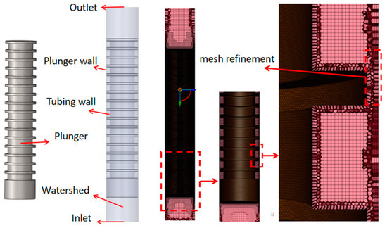
Figure 5.
Plunger Modeling Model.
In this study, the boundary conditions were determined based on the experimental conditions. The fourth set of experimental data was randomly selected for data assimilation, while the remaining sets were used to validate the assimilation results. The SIMPLE algorithm was adopted for pressure–velocity coupling, and the convective terms were discretized using the first-order upwind scheme. The simulation was considered converged when either the inlet flow rate remained unchanged for more than 2000 iterations or the maximum residual of all monitored variables dropped below 1 × 10⁻⁵. The detailed settings are provided in Table 3.
Table 3.
Model and boundary settings.
DA using the EnKF method requires the configuration of several key hyperparameters as follows: the number of ensemble samples, the range of adjustment coefficients, and the variance of specific Gaussian noise. Properly setting these hyperparameters is critical, as inappropriate values may lead to issues such as excessive computational costs, significant deviations of calibration results from experimental values, and instability in data assimilation outcomes. Therefore, hyperparameters must be carefully selected to ensure the accuracy and stability of the data assimilation process.
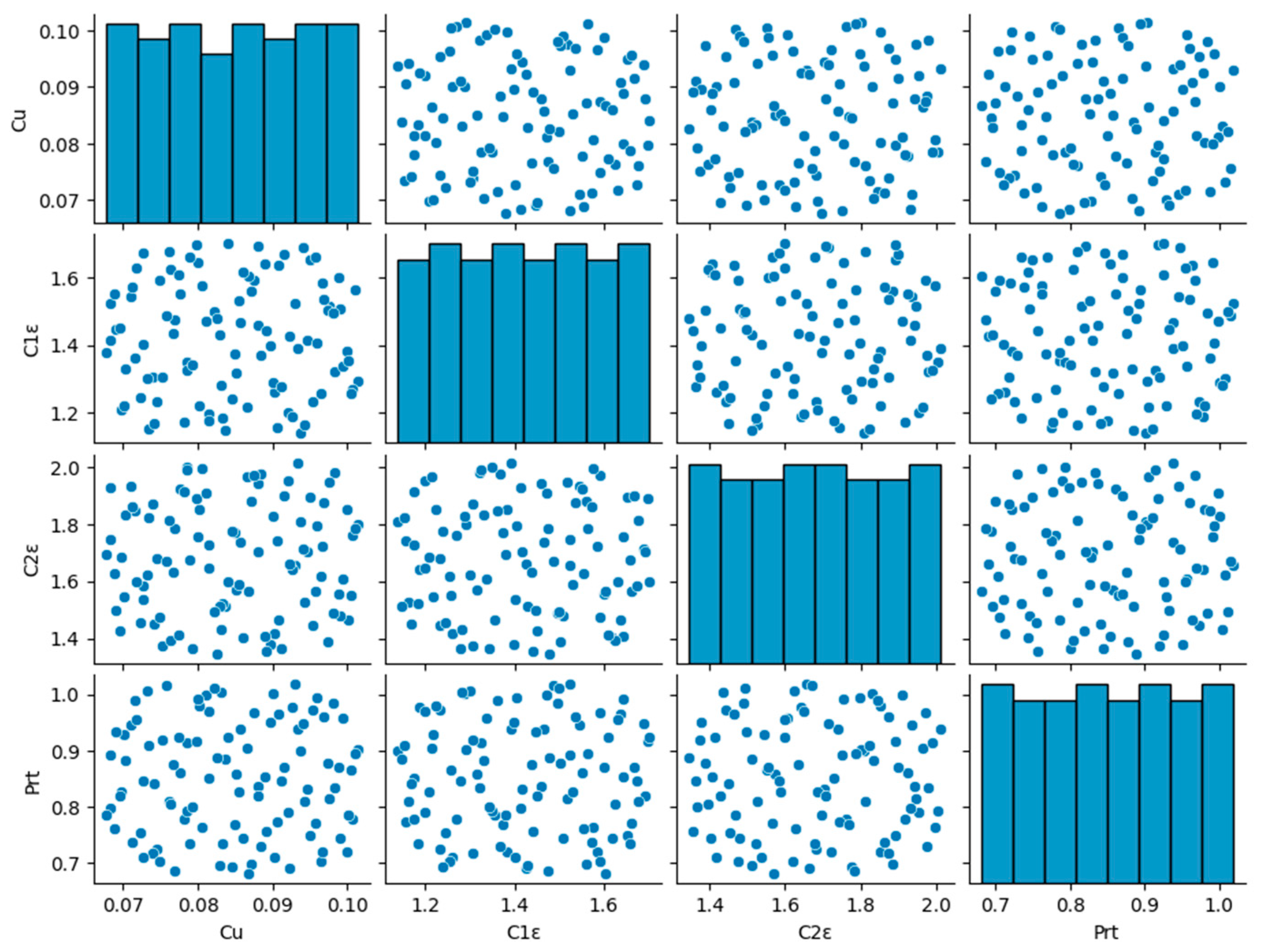
In this study, the optimized Latin Hypercube Sampling (OLHS) method was employed to generate random samples of four turbulence model constants in the RNG k-ε model. The sampling range for each parameter was set to ±20% of its nominal value, specifically 0.0676 ≤ Cu ≤ 0.1014, 1.136 ≤ C1ε ≤ 1.704, 1.344 ≤ C2ε ≤ 2.016, 0.68 ≤ Prt ≤ 1.02.
By evenly dividing each parameter range and optimizing the sample distribution, a total of 100 representative turbulence model sample sets were constructed. As illustrated in Figure 6, the optimized samples were evenly distributed across the high-dimensional parameter space, effectively avoiding clustering and ensuring both the uniformity and representativeness of the sample set.

Figure 6.
Distribution Status of Constant Sample Group.
The 100 sets of turbulence model constants obtained through OLHS were individually input into Fluent for parameter modification, followed by numerical simulations to generate the forecast dataset required for the data assimilation process. In setting the boundary conditions, the bottom-hole pressure and wellhead pressure from the fourth experimental group were randomly selected and applied as the pressure inlet and pressure outlet, respectively, in the simulations. The predicted flow rates corresponding to each set of turbulence model constants were obtained through the simulations. Detailed results are provided in Appendix A.
The observation noise, which is set with a mean of zero and follows a normal distribution with a standard deviation of 0.1, requires careful consideration when determining its variance. This is because the measurement bias includes both the uncertainty inherent in the experimental instrumentation and the biases arising from physical differences between the experimental setup and the predictive model.
5. Analysis of Results
5.1. Data Assimilation Results
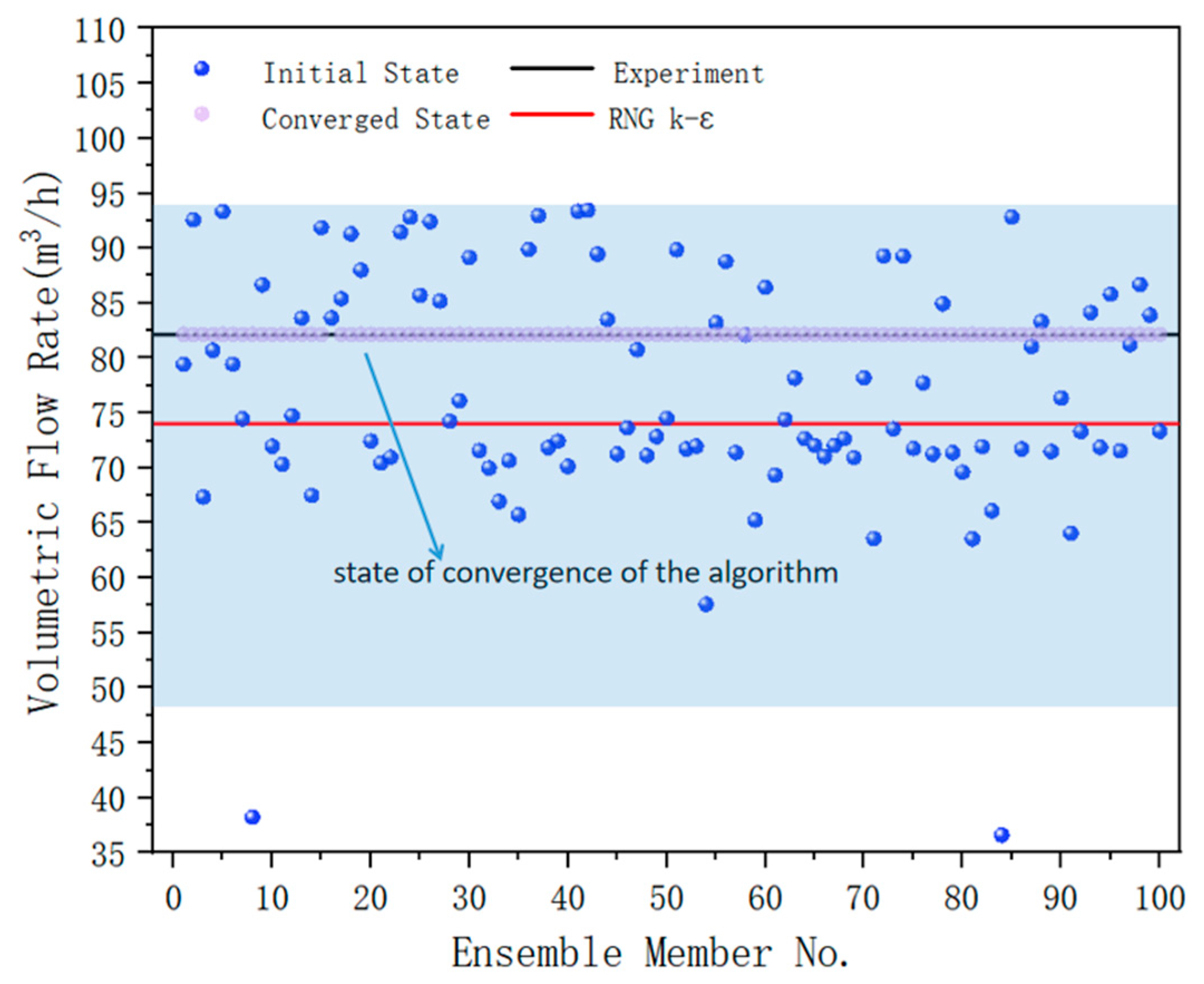
Initially, the generated sample parameter set is input into the FLUENT commercial software (ANSYS 2021 R1)and analyzed using the RNG k-ε turbulence model. The results are subsequently post-processed to derive the initial sample prediction set, as shown in Figure 7. From Figure 7, it is evident that the experimental measurements fall within the range of the predicted sample set. This indicates that the initial sample set captures sufficient information about the flow field, thereby validating the assimilation process. When the EnKF algorithm reaches a converged state, the distribution of all ensemble members closely aligns with the experimental data.
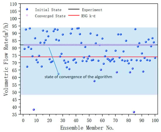
Figure 7.
CFD calculation results.
Subsequently, the initial sample collection and experimental data are integrated using the EnKF algorithm to compute the updated model constants. Table 4 presents both the original and updated constants of the RNG k-ε turbulence model. The results show that after the EnKF integration, constants , , and were modified relative to their initial values, while constant remained largely unchanged.
Table 4.
Model constants for models before and after data assimilation.
The Mean Squared Error (MSE) quantifies the deviation between experimental measurements and theoretical values. A smaller MSE indicates higher accuracy of the experimental results. In this study, a lower MSE between the predicted flow rate from the turbulence model and the experimental flow rate reflects greater predictive accuracy of the corresponding model.
The definition of MSE is as follows:
: Sample size
: The i-th predicted value.
: The i-th true value.
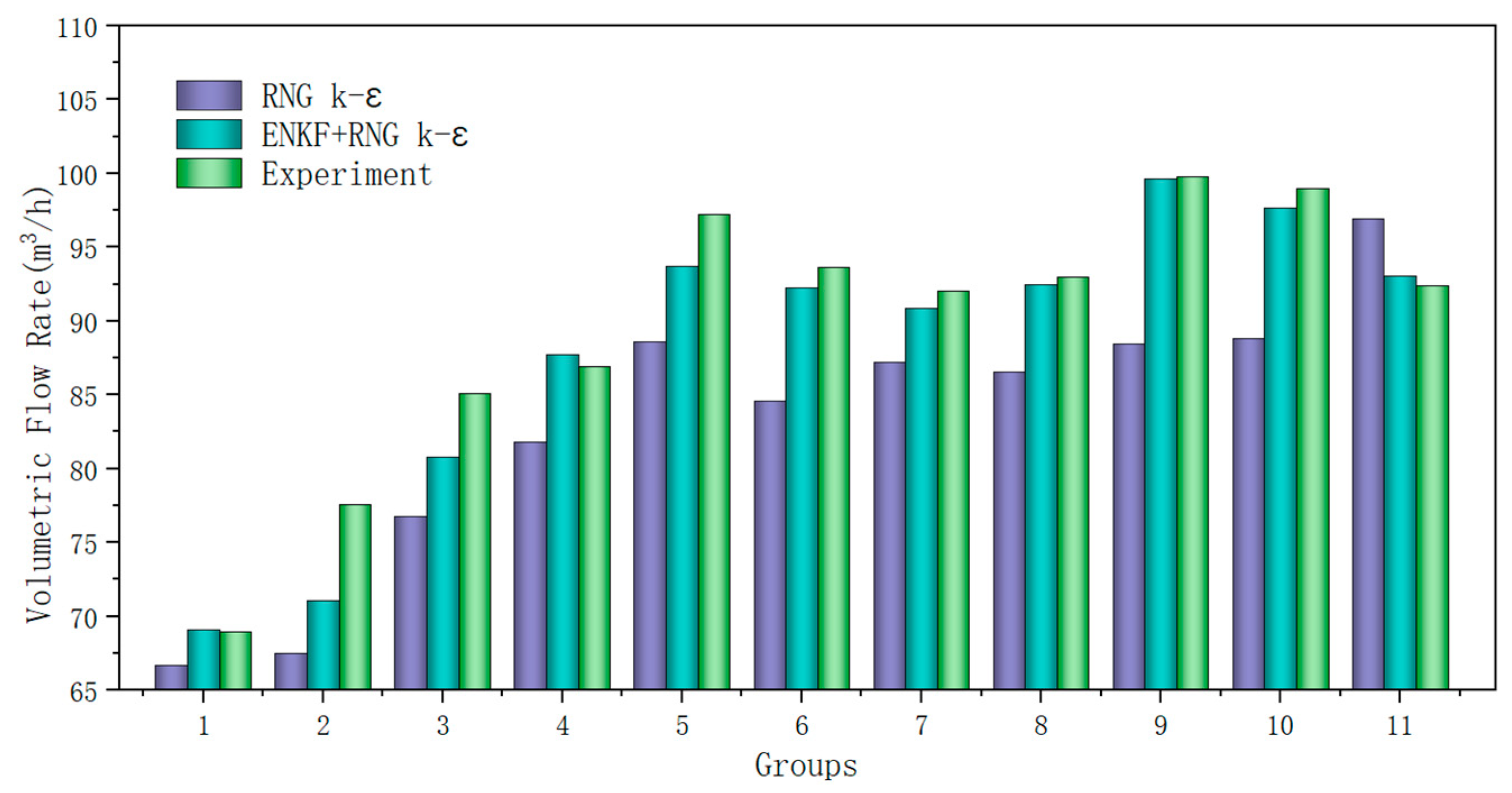
Using the data-assimilated RNG k-ε model to predict the flow rate of the air-lift plunger under various operating conditions and comparing it with the predictions from the original constant RNG k-ε model, as shown in Figure 8, it is evident that the accuracy of the assimilated turbulence model has significantly improved. In addition, after data assimilation, the turbulence model exhibits high prediction accuracy for the original rectangular slot plunger case and shows significantly improved accuracy for the circular arc-shaped slot plunger, as illustrated in Figure 9. The mean square errors of the RNG k-ε model before and after assimilation are detailed in Table 5, showing a decrease from 60.67 and 61.48 to 7.12 and 7.20 for the rectangular and circular arc plungers, respectively. The recalibrated model demonstrates robust scalability and effectively predicts the sealing performance of turbulent sealing plungers with various groove types across different operating conditions, thereby significantly enhancing the accuracy of these predictions.
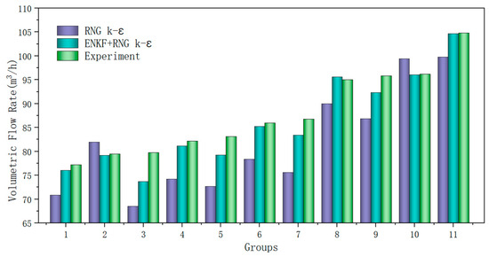
Figure 8.
Comparison of predicted and experimental flows from the rectangular slot plunger RNG k-ε model and the ENKF+RNG k-ε model.
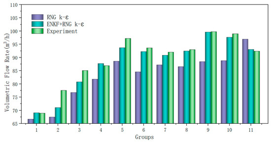
Figure 9.
Comparison of predicted and experimental flow rates of circular grooved plunger RNG k-ε model and ENKF+RNG k-ε model.
Table 5.
Mean square Error (MSE) before and after data assimilation.
5.2. Flow Field Analysis
Figure 10 shows the velocity contour in the Y-direction on the YZ cross-section, illustrating a significant phenomenon. Before data assimilation, the positive and negative flows in the Y-direction are dispersed. After DA, a large-scale circumferential flow emerges in the slot.
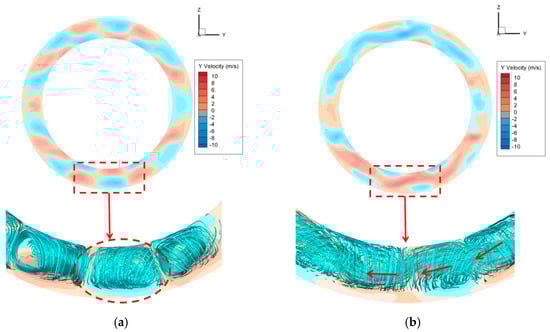
Figure 10.
(a) Y-direction velocity cloud before data assimilation. (b) Y-direction velocity cloud after data assimilation.
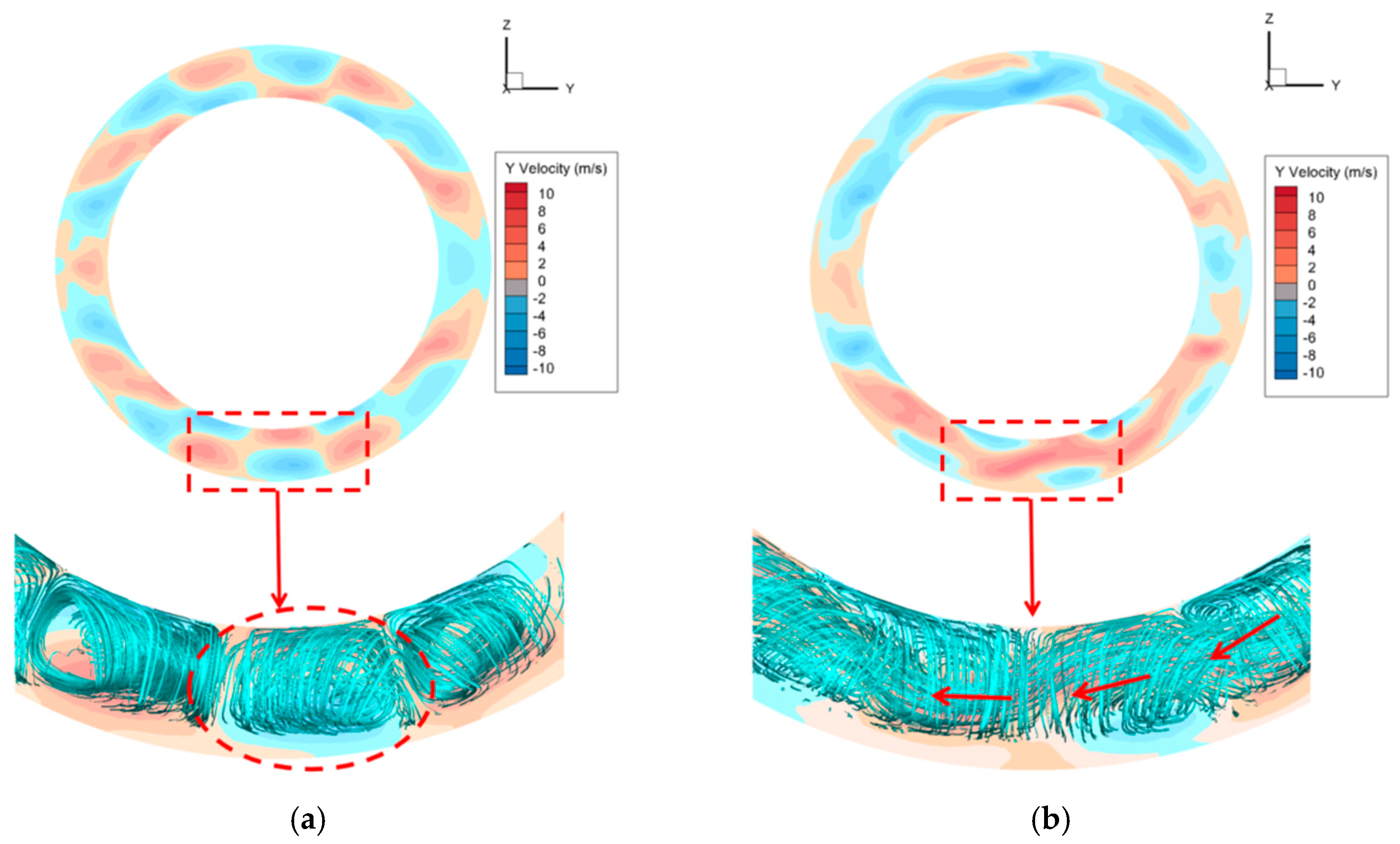
Figure 11 depicts the significant changes in the 3D flow trajectories within the plunger groove before and after DA. Initially, as shown in Figure 11a, the flow trajectories exhibit clustered vortices, with adjacent vortices displaying opposing velocities in the Y-direction and minimal radial flow. After assimilation, Figure 11b shows that, while the original vortex structures are retained, these vortices transform into structures with extensive radial flow.
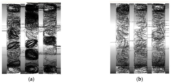
Figure 11.
(a) Streamlines before data assimilation. (b) Streamlines after data assimilation.
The circumferential motion of the fluid in the axial cross-section is perpendicular to the inflow direction and is significantly influenced by the circumferential velocity. This interaction results in a more complex airflow pattern within the plunger gap. Specifically, the circumferential motion of the fluid combines with the axial inflow velocity, generating intricate vortex structures. This complex flow pattern may influence the sealing performance of the plunger. The increased flow complexity could lead to variations in turbulence intensity within the plunger gap, thereby affecting the sealing effectiveness. Whether this impact enhances or diminishes the plunger’s sealing effectiveness requires further detailed analysis.
As shown in Figure 12, this phenomenon is not limited to the second groove but is observed in all grooves of the plunger, ruling out the possibility of chance. The consistency of this phenomenon indicates that the flow changes induced by data assimilation follow a general rule rather than being isolated events. This further demonstrates the effectiveness and stability of data assimilation in improving fluid flow characteristics. Since this phenomenon occurs in all grooves, it suggests that data assimilation can produce significant flow optimization effects across different structural regions. This consistent flow pattern contributes to enhancing the overall performance and reliability of the system.
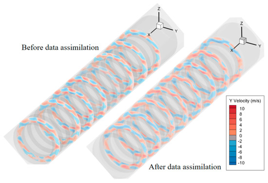
Figure 12.
Plunger overall Y-direction velocity cloud.
Figure 13 illustrates the distribution of vortex magnitude on the surface before and after DA. The vortex magnitude reflects the rotational curl of the vortex velocity vector, enabling the assessment of the vortex’s intensity and directional orientation. A larger vortex magnitude indicates higher fluid velocities, increased energy consumption, and greater fluid dissipation, all of which positively influence the sealing performance of the plunger. The figure shows that post-DA, the vortex magnitude is reduced compared to pre-DA levels. Analysis of the flow diagram reveals smaller vortex magnitudes in regions with circumferential flow of the flow slugs and larger magnitudes in areas opposing the vortex rotation.
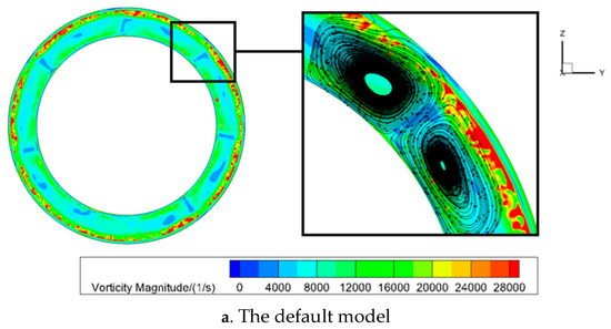
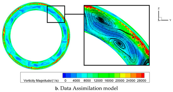
Figure 13.
Vorticity contour maps of the same cross section.
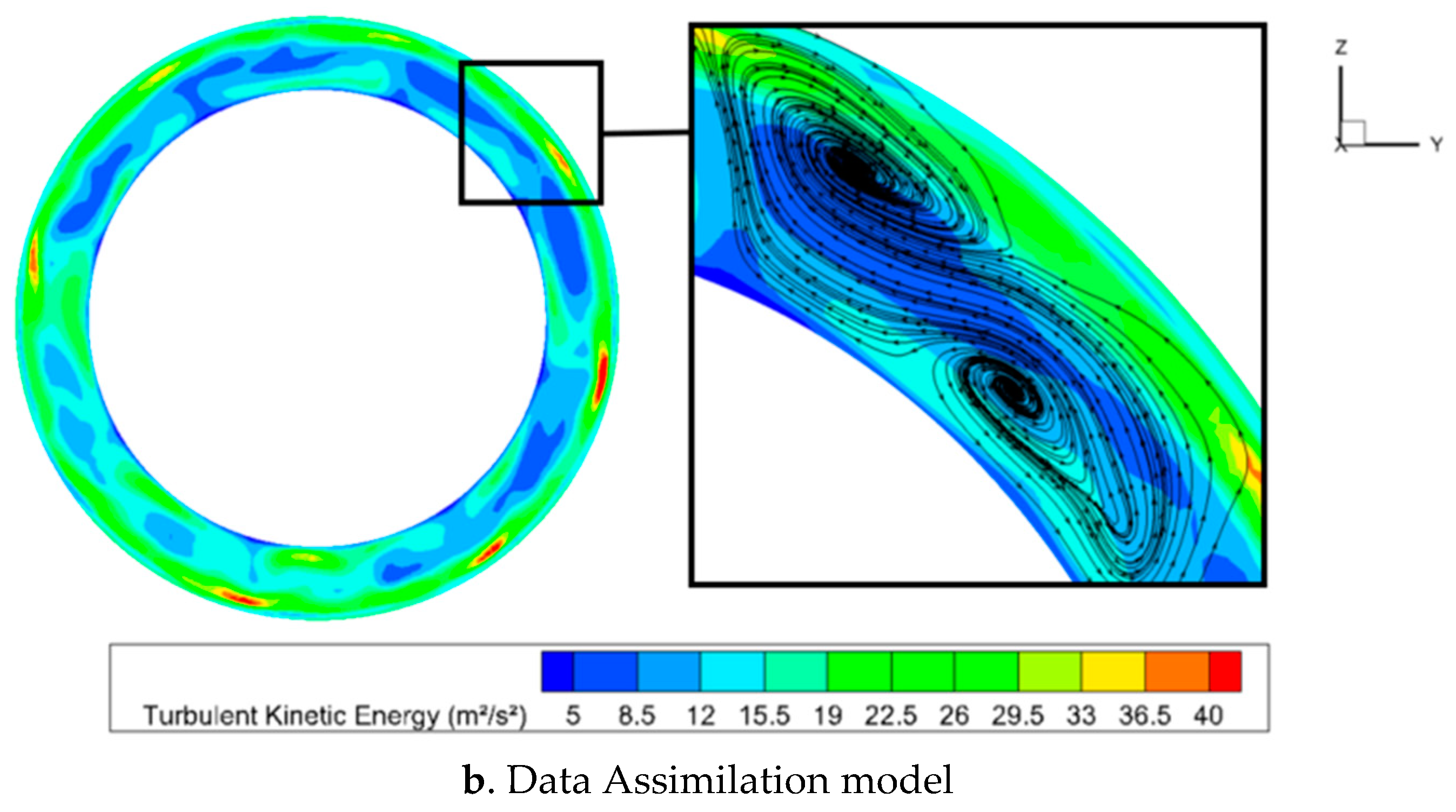
Figure 14 illustrates the distribution of turbulent kinetic energy, which aligns with the vortex magnitude distribution. Turbulent kinetic energy, an indicator of turbulence intensity within the fluid, is typically directly related to the fluid’s dynamic activity and energy exchange. Lower turbulent kinetic energy indicates weaker fluid dynamics, which could negatively affect the sealing performance of the plunger. Post-DA, the overall level of turbulent kinetic energy is observed to decrease. While this reduction may stabilize fluid flow, moderate turbulence is essential for effective sealing between the plunger and the pipeline; hence, reduced turbulent kinetic energy might compromise seal integrity. The flow diagram reveals that in regions with low turbulent kinetic energy, the fluid exhibits distinct circumferential flow characteristics. This flow pattern suggests a general reduction in turbulence intensity, potentially impairing the sealing performance of the plunger.
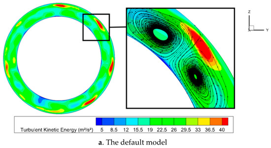
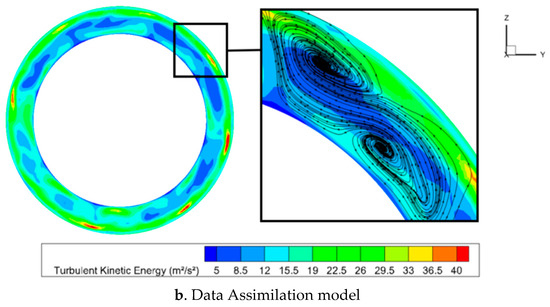
Figure 14.
Turbulent kinetic energy contour maps of the same cross section.
Figure 15 depicts the distribution of turbulent kinetic energy dissipation rate, which aligns with the patterns observed in the previous turbulent kinetic energy and vortex magnitude distributions. The turbulent kinetic energy dissipation rate, a metric for quantifying the rate of turbulence energy loss in a fluid, is crucial for understanding and optimizing the efficiency of fluid dynamic systems. Post-DA, a reduction in the overall level of turbulent kinetic energy dissipation rate is observed. However, for plunger systems that rely on fluid dynamic pressure to maintain seals, a lower dissipation rate may indicate insufficient fluid dynamics, potentially compromising the sealing performance of the plunger.
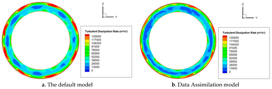
Figure 15.
Dissipation rate of turbulent kinetic energy contour maps of the same cross section.
Precise control of fluid dynamic characteristics is crucial for optimizing plunger systems. Studies have shown that significant circumferential flow may exist in the actual flow through the plunger gap, and previous numerical simulations may have overestimated the sealing performance of the plunger. Therefore, by reducing circumferential flow and simultaneously increasing vortex intensity, turbulent kinetic energy, and turbulent dissipation rate, the sealing efficiency and overall performance of the plunger system can be significantly improved. These optimization measures not only enhance the sealing effect of the plunger but also improve the stability and efficiency of the gas lift process, leading to higher production efficiency.
6. Conclusions
This study applied the Ensemble Kalman Filter (EnKF) data assimilation technique to calibrate the constants of the RNG k-ε turbulence model, aiming to improve the predictive accuracy of gas flow through plunger lift systems. The integration of experimental observations with numerical simulations enabled significant reductions in prediction errors. Specifically, the mean square error (MSE) for the rectangular and circular arc plungers decreased from 60.67 and 61.48 to 7.12 and 7.20, respectively, demonstrating the method’s robustness and adaptability to different plunger geometries.
In addition to quantitative improvements, data assimilation revealed critical insights into the flow characteristics within the plunger gap. Notably, changes in the circumferential flow structures and turbulence intensity indicated that conventional models may overestimate sealing performance. The recalibrated model better captured these complex features, providing a more realistic representation of the underlying physics.
The findings highlight the effectiveness of data assimilation not only in enhancing model fidelity but also in improving the understanding of gas–liquid interaction mechanisms in narrow annular flows. This approach provides a new methodology and perspective for optimizing the geometric design of plunger slot structures, allowing for better evaluation of sealing performance and flow behavior under varying operational conditions.
From an application standpoint, the calibrated turbulence model offers practical guidance for the structural optimization of gas-lift plungers, particularly in the design and assessment of different sealing slot types. Future research will focus on extending the assimilation framework to incorporate multi-parameter uncertainty quantification and to explore more diverse plunger configurations in low-pressure gas wells.
Author Contributions
Methodology and Field Experiments: J.Z. and Y.S.; Data Analysis and Original Draft Preparation: J.Z. Y.S.; Review and Editing, Project Management, and Funding Acquisition: J.Z.; Resources and Supervision: Y.X.; Manuscript Organization and Experiment Coordination: Y.Y. and J.W. All authors have read and agreed to the published version of the manuscript.
Funding
This research received no external funding.
Institutional Review Board Statement
Not applicable.
Informed Consent Statement
Not applicable.
Data Availability Statement
The datasets generated during and/or analyzed during this current study are available from the corresponding author upon reasonable request.
Conflicts of Interest
The authors declare no conflicts of interest.
Appendix A
| Cu | C1ε | C2ε | Prt | Q (m3/h) | Cu | C1ε | C2ε | Prt | Q (m3/h) |
| 0.09885 | 1.5996 | 1.5535 | 0.87 | 79.41 | 0.07521 | 1.3056 | 1.3729 | 0.9191 | 89.86 |
| 0.06878 | 1.553 | 1.6286 | 0.7613 | 92.56 | 0.08454 | 1.2389 | 1.7762 | 0.6928 | 71.72 |
| 0.09985 | 1.3818 | 1.8535 | 0.7212 | 67.34 | 0.0734 | 1.1527 | 1.8236 | 0.9102 | 71.98 |
| 0.0732 | 1.2997 | 1.6233 | 1.0076 | 80.70 | 0.10052 | 1.2571 | 1.5511 | 0.8649 | 57.58 |
| 0.07631 | 1.6256 | 1.3953 | 0.8048 | 93.34 | 0.088 | 1.6916 | 1.7061 | 0.8206 | 83.22 |
| 0.09403 | 1.6882 | 1.7141 | 0.9473 | 79.43 | 0.07261 | 1.4011 | 1.5356 | 0.7102 | 88.79 |
| 0.07769 | 1.5513 | 1.925 | 0.8613 | 74.46 | 0.08489 | 1.3728 | 1.7696 | 0.7675 | 71.39 |
| 0.07095 | 1.5452 | 1.935 | 0.9451 | 38.21 | 0.09741 | 1.5018 | 1.388 | 0.8775 | 82.11 |
| 0.06768 | 1.3789 | 1.697 | 0.7852 | 86.65 | 0.10135 | 1.2917 | 1.8019 | 0.9028 | 65.25 |
| 0.08372 | 1.1464 | 1.5126 | 0.8853 | 71.98 | 0.08915 | 1.4424 | 1.3547 | 0.7557 | 86.42 |
| 0.07813 | 1.1734 | 1.917 | 0.7771 | 70.31 | 0.08846 | 1.3688 | 1.9757 | 0.7286 | 69.35 |
| 0.09297 | 1.5229 | 1.6545 | 1.0186 | 74.73 | 0.07036 | 1.3305 | 1.8341 | 0.883 | 74.41 |
| 0.07016 | 1.2186 | 1.5439 | 0.9289 | 83.63 | 0.09118 | 1.2776 | 1.3636 | 0.8452 | 78.15 |
| 0.09057 | 1.1568 | 1.7421 | 0.7746 | 67.49 | 0.07845 | 1.3504 | 2.0031 | 0.7923 | 72.68 |
| 0.08253 | 1.4789 | 1.3455 | 0.8885 | 91.87 | 0.08025 | 1.2221 | 1.8523 | 0.9807 | 72.04 |
| 0.07669 | 1.4366 | 1.6333 | 0.8752 | 83.67 | 0.09458 | 1.4164 | 1.7024 | 0.8305 | 71.02 |
| 0.08671 | 1.604 | 1.5675 | 0.6802 | 85.41 | 0.0969 | 1.5363 | 1.8744 | 0.9604 | 72.05 |
| 0.08605 | 1.6178 | 1.4031 | 0.7442 | 91.30 | 0.07861 | 1.3251 | 1.9904 | 0.9138 | 72.66 |
| 0.08212 | 1.5006 | 1.4918 | 1.0123 | 87.99 | 0.09938 | 1.3365 | 1.6071 | 0.9576 | 70.93 |
| 0.08335 | 1.1829 | 1.5227 | 0.7347 | 72.45 | 0.07688 | 1.474 | 1.7835 | 0.6854 | 78.17 |
| 0.09429 | 1.1623 | 1.5257 | 0.8093 | 70.42 | 0.09831 | 1.3212 | 1.9809 | 0.8341 | 63.58 |
| 0.08154 | 1.1978 | 1.6473 | 0.9703 | 70.98 | 0.09085 | 1.6366 | 1.4628 | 0.9641 | 89.28 |
| 0.08901 | 1.6421 | 1.4067 | 0.8542 | 91.46 | 0.08565 | 1.4664 | 1.7382 | 0.9381 | 73.56 |
| 0.06907 | 1.4484 | 1.4981 | 0.9326 | 92.84 | 0.07918 | 1.3417 | 1.3654 | 0.8003 | 89.26 |
| 0.07572 | 1.4859 | 1.6692 | 1.0154 | 85.72 | 0.09531 | 1.233 | 1.4435 | 0.9726 | 71.76 |
| 0.07478 | 1.5907 | 1.4736 | 0.7039 | 92.40 | 0.09905 | 1.5092 | 1.4793 | 0.7451 | 77.73 |
| 0.07995 | 1.6444 | 1.7555 | 0.9912 | 85.18 | 0.09501 | 1.6538 | 1.894 | 0.7486 | 71.26 |
| 0.08509 | 1.3162 | 1.5724 | 0.8581 | 74.25 | 0.07116 | 1.5734 | 1.8635 | 0.738 | 84.93 |
| 0.06828 | 1.4148 | 1.9308 | 0.7986 | 76.09 | 0.09149 | 1.6678 | 1.9001 | 0.8706 | 71.39 |
| 0.07884 | 1.6602 | 1.677 | 0.7338 | 89.16 | 0.09 | 1.2888 | 1.831 | 1.001 | 69.62 |
| 0.08743 | 1.5926 | 1.9705 | 0.9671 | 71.58 | 0.09199 | 1.2004 | 1.9542 | 0.7893 | 63.53 |
| 0.09253 | 1.1876 | 1.6413 | 0.9784 | 70.01 | 0.08061 | 1.575 | 1.9977 | 0.7626 | 71.94 |
| 0.09327 | 1.3919 | 2.0132 | 0.9384 | 66.94 | 0.08656 | 1.2149 | 1.9666 | 0.9052 | 66.10 |
| 0.09643 | 1.2552 | 1.6186 | 0.7029 | 70.67 | 0.07447 | 1.2315 | 1.6814 | 0.7258 | 36.59 |
| 0.10075 | 1.2687 | 1.7611 | 0.7793 | 65.74 | 0.0727 | 1.675 | 1.5831 | 0.8472 | 92.82 |
| 0.06822 | 1.5249 | 1.749 | 0.8925 | 89.87 | 0.08718 | 1.5605 | 1.8834 | 0.6993 | 71.74 |
| 0.07178 | 1.6308 | 1.5991 | 0.9543 | 92.95 | 0.08307 | 1.2824 | 1.4335 | 1.005 | 81.07 |
| 0.10019 | 1.3541 | 1.4663 | 0.7862 | 71.84 | 0.08967 | 1.3972 | 1.3779 | 0.9504 | 83.29 |
| 0.08798 | 1.4581 | 1.9428 | 0.8373 | 72.45 | 0.10113 | 1.5643 | 1.7879 | 0.8946 | 71.49 |
| 0.09754 | 1.5164 | 1.9473 | 0.8144 | 70.12 | 0.09817 | 1.495 | 1.491 | 0.9839 | 76.36 |
| 0.07738 | 1.6106 | 1.4116 | 0.9251 | 93.35 | 0.09365 | 1.1379 | 1.8083 | 0.9008 | 64.07 |
| 0.06953 | 1.4513 | 1.4276 | 0.8187 | 93.47 | 0.0811 | 1.4718 | 1.9113 | 0.9992 | 73.31 |
| 0.08396 | 1.7017 | 1.5969 | 0.9246 | 89.46 | 0.08283 | 1.4294 | 1.5104 | 0.696 | 84.15 |
| 0.0854 | 1.5311 | 1.5876 | 0.8259 | 83.50 | 0.07403 | 1.3072 | 1.8732 | 0.7168 | 71.87 |
| 0.09224 | 1.4251 | 1.6634 | 0.6901 | 71.26 | 0.07608 | 1.6779 | 1.813 | 0.8088 | 85.80 |
| 0.07153 | 1.3613 | 1.8456 | 0.9887 | 73.64 | 0.08146 | 1.1759 | 1.728 | 0.8503 | 71.55 |
| 0.07413 | 1.1692 | 1.4489 | 0.8416 | 80.75 | 0.07982 | 1.6989 | 1.891 | 0.9178 | 81.22 |
| 0.09589 | 1.4052 | 1.7971 | 0.9941 | 71.14 | 0.07235 | 1.2453 | 1.453 | 0.7535 | 86.68 |
| 0.06976 | 1.2094 | 1.6869 | 0.8279 | 72.85 | 0.09568 | 1.6607 | 1.5643 | 0.7698 | 83.90 |
| 0.0902 | 1.2618 | 1.4182 | 0.7113 | 74.52 | 0.09668 | 1.5852 | 1.7215 | 0.7194 | 73.35 |
References
- Chen, D.; Yao, Y.; Fu, G.; Meng, H.; Xie, S. A new model for predicting liquid loading in deviated gas wells. J. Nat. Gas Sci. Eng. 2016, 34, 178–184. [Google Scholar] [CrossRef]
- Waltrich, P.J.; Posada, C.; Martinez, J.; Falcone, G.; Barbosa, J.R., Jr. Experimental investigation on the prediction of liquid loading initiation in gas wells using a long vertical tube. J. Nat. Gas Sci. Eng. 2015, 26, 1515–1529. [Google Scholar] [CrossRef]
- Luo, S.; Kelkar, M. Effective method to predict installation of plunger in a gas well. J. Energy Resour. Technol. 2014, 136, 024501. [Google Scholar] [CrossRef]
- Zhao, K.; Mu, L.; Tian, W.; Bai, B. Gas-liquid flow seal in the smooth annulus during plunger lifting process in gas wells. J. Nat. Gas Sci. Eng. 2021, 95, 104195. [Google Scholar] [CrossRef]
- Duraisamy, K.; Iaccarino, G.; Xiao, H. Turbulence modeling in the age of data. Annu. Rev. Fluid Mech. 2019, 51, 357–377. [Google Scholar] [CrossRef]
- Wunsch, C. The Ocean Circulation Inverse Problem; Cambridge University Press: Cambridge, UK, 1996; p. 422. [Google Scholar]
- Lynch, P. The origins of computer weather prediction and climate modeling. J. Comput. Phys. 2008, 227, 3431–3444. [Google Scholar] [CrossRef]
- Fan, X.P.; Qu, G.; Liu, Y.F. Bridge extreme stress prediction based on new data assimilation algorithm. J. Bridge Eng. 2020, 50, 572–580. [Google Scholar] [CrossRef]
- Kato, H.; Yoshizawa, A.; Ueno, G.; Obayashi, S. A data assimilation methodology for reconstructing turbulent flows around aircraft. J. Comput. Phys. 2015, 283, 559–581. [Google Scholar] [CrossRef]
- Deng, Z.; He, C.; Wen, X.; Liu, Y. Recovering turbulent flow field from local quantity measurement: Turbulence modeling using ensemble-Kalman-filter-based data assimilation. J. Vis. 2018, 21, 1043–1063. [Google Scholar] [CrossRef]
- Zhang, X.L.; Michelén-Ströfer, C.; Xiao, H. Regularized ensemble Kalman methods for inverse problems. J. Comput. Phys. 2020, 416, 109517. [Google Scholar] [CrossRef]
- He, X.; Yuan, C.; Gao, H.; Chen, Y.; Zhao, R. Calibration of Turbulent Model Constants Based on Experimental Data Assimilation: Numerical Prediction of Subsonic Jet Flow Characteristics. Sustainability 2023, 15, 10219. [Google Scholar] [CrossRef]
- Fang, P.; He, C.; Wang, P.; Xu, S.; Liu, Y. Data assimilation of steam flow through a control valve using ensemble Kalman filter. J. Fluids Eng. 2021, 143, 091201. [Google Scholar] [CrossRef]
- Liu, T.; Li, R.; Gao, L.; Zhao, L. Experimental data-driven cascade flow field prediction based on data assimilation. Acta Aeronaut. Astronaut. Sin. 2023, 44, 112–127. [Google Scholar]
- Yu, J.; Qiu, H.; Jiao, Y.; Tian, Y.; Meng, Y.; Wang, W.; Li, X. Numerical prediction of heat transfer performance of plate heat exchanger based on experimental data assimilation to calibrate turbulence model constants. Therm. Sci. Eng. Prog. 2022, 34, 101433. [Google Scholar] [CrossRef]
- Meng, L.; Yang, J.; Yang, H. Research on data assimilation of wind turbine airfoils in stall. Acta Aerodyn. Sin. 2024, 42, 37–45. [Google Scholar]
- Tang, Y.; Liang, Z. A new method of plunger lift dynamic analysis and optimal design for gas well deliquification. In Proceedings of the SPE Annual Technical Conference and Exhibition, Denver, CO, USA, 21–24 September 2008. SPE-116764. [Google Scholar] [CrossRef]
- Ren, Z.A.; Hao, D.; Xie, H.J. Several turbulence models and their applications in FLUENT. Chem. Equip. Technol. 2009, 30, 39–43. [Google Scholar] [CrossRef]
- Evensen, G. Sequential data assimilation with a nonlinear quasi-geostrophic model using Monte Carlo methods to forecast error statistics. J. Geophys. Res. Oceans 1994, 99, 10143–10162. [Google Scholar] [CrossRef]
- Ligęza, P. Constant-Temperature Anemometer Bandwidth Shape Determination for Energy Spectrum Study of Turbulent Flows. Energies 2021, 14, 4495. [Google Scholar] [CrossRef]
- Maas, H.G.; Grün, A.; Papantoniou, D. Particle tracking velocimetry in three-dimensional flows. Exp. Fluids 1993, 15, 133–146. [Google Scholar] [CrossRef]
- Zhao, K.; Tian, W.; Li, X.; Bai, B. A physical model for liquid leakage flow rate during plunger lifting process in gas wells. J. Nat. Gas Sci. Eng. 2018, 49, 32–40. [Google Scholar] [CrossRef]
- Wang, Z.; Liu, C.; Liu, C.; Xu, H.; Zhang, J.; Cao, M. Calculation and analysis of sealing performance on the outer wall of gas-lift plungers. Earthq. Eng. Eng. Vib. 2019, 39, 7–17. [Google Scholar] [CrossRef]


Disclaimer/Publisher’s Note: The statements, opinions and data contained in all publications are solely those of the individual author(s) and contributor(s) and not of MDPI and/or the editor(s). MDPI and/or the editor(s) disclaim responsibility for any injury to people or property resulting from any ideas, methods, instructions or products referred to in the content. |
© 2025 by the authors. Licensee MDPI, Basel, Switzerland. This article is an open access article distributed under the terms and conditions of the Creative Commons Attribution (CC BY) license (https://creativecommons.org/licenses/by/4.0/).