Acoustic Emission-Based Method for IFSS Characterization in Single-Fiber Fragmentation Tests

Abstract

Carbon fiber-reinforced polymers (CFRP) are widely used composite materials in structural applications, where their mechanical performance is significantly influenced by interfacial shear strength (IFSS). The single fiber fragmentation test (SFFT) is a common technique for characterizing IFSS, but its reliance on optical microscopy makes it time-consuming and impractical for opaque matrices. This study presents an alternative methodology based on acoustic emission (AE) analysis, enabling the estimation of fragment lengths through statistical modeling. The AE technique captures the energy released during fiber fragmentation, represented as AE bursts, whose accurate detection is crucial. A signal-processing approach based on progressive simplification enhances burst detection. To refine the estimation of fragment lengths, a gamma distribution is fitted to experimental data, accounting for observed asymmetry in optical measurements. Results indicate that this approach achieves an IFSS determination error of 14.16% at a 95% confidence level. This study demonstrates the feasibility of using AE for IFSS characterization in SFFT and contributes to future research on AE applications in composite materials.

1. Introduction

Carbon fiber reinforced polymers (CFRP) are constituted by the heterogeneous bonding of carbon fiber (CF) and a thermoplastic polymeric matrix. These materials stand out in the structural field due to their excellent mechanical performance, such as high specific strength, and high specific stiffness [1]. Currently, their applications are found in multiple fields, such as automotive, aerospace, energy, and others. However, its implementation is limited to the level of adhesion between the carbon fiber and its matrix, making it crucial to study the properties and mechanical behavior [2].

The interaction between the fiber and matrix can be quantified by measuring the interfacial shear strength (IFSS); this is one of the most important properties for the correct performance of composite materials, since it directly influences the effective transfer and uniform distribution of loads between the matrix and the reinforcement, limiting the strength and toughness of the final composite [3,4]. This parameter is mainly affected by hydroxyl and carboxylic functional groups on the fiber surface and interlocking caused by fiber morphology [5]. In the literature, several surface treatments have been proposed to improve fiber–matrix adhesion, including oxidation processes, plasma and laser treatments [6,7], sizing [8,9], chemical vapor deposition [9], and other multiscale reinforcements [10,11,12].

Due to the critical role of IFSS in composite performance, the mechanical characterization of interfacial bonding has become a subject of considerable research interest. Over the past decades, several techniques have been developed to quantify this parameter and are classified into microscale and macroscale approaches. Microscale methods include the micro bond-test [13], single fiber pull-out [14], single fiber push-out [15], and single fiber fragmentation test [16,17,18]. These techniques enable the decomposition of the composite’s overall behavior into simplified fiber–matrix interactions, allowing a more isolated study of adhesion mechanisms. Identifying key interfacial parameters—such as IFSS, interfacial fracture toughness (IFFT), and coefficient of interfacial friction ($u_i$)—is crucial, as it enables the analysis and description of interfacial debonding and fracture processes in composite materials through numerical simulations and analytical models [5,19].

Complementary to these microscale techniques, meso- and macroscale methods have emerged as a convenient alternative for the indirect evaluation of interfacial shear strength, particularly due to their lower experimental complexity. Among the most reported are the transverse tensile test [13], 45° tension test [20], fiber bundle pull-out test [3], and Iosipescu shear test [21].

Among the microscale methods, the single fiber fragmentation technique (SFFT) is the simplest to implement in terms of instrumentation, as it requires basic microscopes and universal testing machines. This method consists of a fiber embedded in a straight or dog bone-shaped matrix subjected to a controlled tensile state. This generates a series of breaks in the fiber until all fragment lengths are within a critical length, thus reaching the so-called saturation status. Conventionally, the number of fragments and the length of the breaks are measured using polarized optical microscopes. For IFSS quantification, a classical approach is to use the Kelly and Tyson equation [22], the main input parameter being the average fragment length. These are measured directly by optical microscopy [16,23,24] being the usual technique or indirectly through acoustic emissions (AE) [25].

The optical method for measuring fragment length requires neat surface treatment and is time-consuming, making it impractical for non-transparent matrices or high adhesion interfaces where the fiber fragments hundreds of times. To address this, acoustic emission techniques have been integrated into SFFT to detect breaks and indirectly calculate the average fragment length [26]. Park et al. [27] used a pair of AE sensors to detect and locate breaks within the SFFT of carbon fibers under different sizing conditions. In their investigation, the AE method generally presented a lower number of ruptures compared to the optical method. They attributed this loss of events to the energy dissipation caused by the damping of the epoxy matrix. Furthermore, they conclude that the AE method, considering the wave velocity and according to the level of matrix defects, performs well for the location of flaws within the specimen. On the other hand, the average fragment length is a key factor for the determination of IFSS. Drzal et al. [28] suggested that since fiber strength varies during testing, Weibull distributions should be used for fragment lengths.

In acoustic emission techniques, burst detection is critical for accurate fracture identification. In burst detection methods, the threshold and its parameters are generally determined by trial and error, with the fixed threshold method being the most widely used due to its simplicity and low computational cost. However, this method has problems when the signal contains multiple high-amplitude bursts in a short period of time. This causes the signal’s noise level to increase above the detection threshold, resulting in multiple bursts being interpreted as a single event, leading to a loss of information and possible interpretation errors [29,30]. Therefore, in this work, the conventional fixed threshold method is not used. Instead, a burst detection method is developed based on the approach proposed by Unnthorsson in [31], which describes a methodology to improve the detectability of AE bursts. In this study, burst detection is performed by simplifying the raw AE signal through a series of smoothing operations until a triangular envelope is obtained, where the appearance of the bursts is represented by a triangle in the envelope. From these triangles, the bursts present in the raw AE signal are identified and extracted separately.

In AE applications, the fragment length cannot be measured directly, so the critical length used is the arithmetic mean estimated from the calibrated length and the number of AE events. In this research, the AE technique is used to obtain the IFSS in SFFTs. For this purpose, single fiber fragmentation specimens are fabricated, and the IFSS is determined using AE and optical microscopy for comparison. Burst detection is performed using the methodology presented by Unnthorsson to improve accuracy. In addition, the mean length correction for the IFSS determination in AE is performed using statistical analysis based on the calibration of a gamma distribution fitted to the reference data, which improves the accuracy of the estimation and reduces the discrepancy with the optical measurement.

2. Materials and Methods

2.1. Materials

The specimens are fabricated from 245 g/m² planar density 2/2 twill carbon fiber (Tenax-E13 HTA40, 200 tex (3k), tensile strength (${\sigma }_f$): 4.0 GPa; R&G Composite Technology, Waldenbuch, Germany), YD-114F Bisphenol-A/F epoxy resin and KH-813 hardener (Kukdo Chemical Co., Seúl, Republic of Korea).

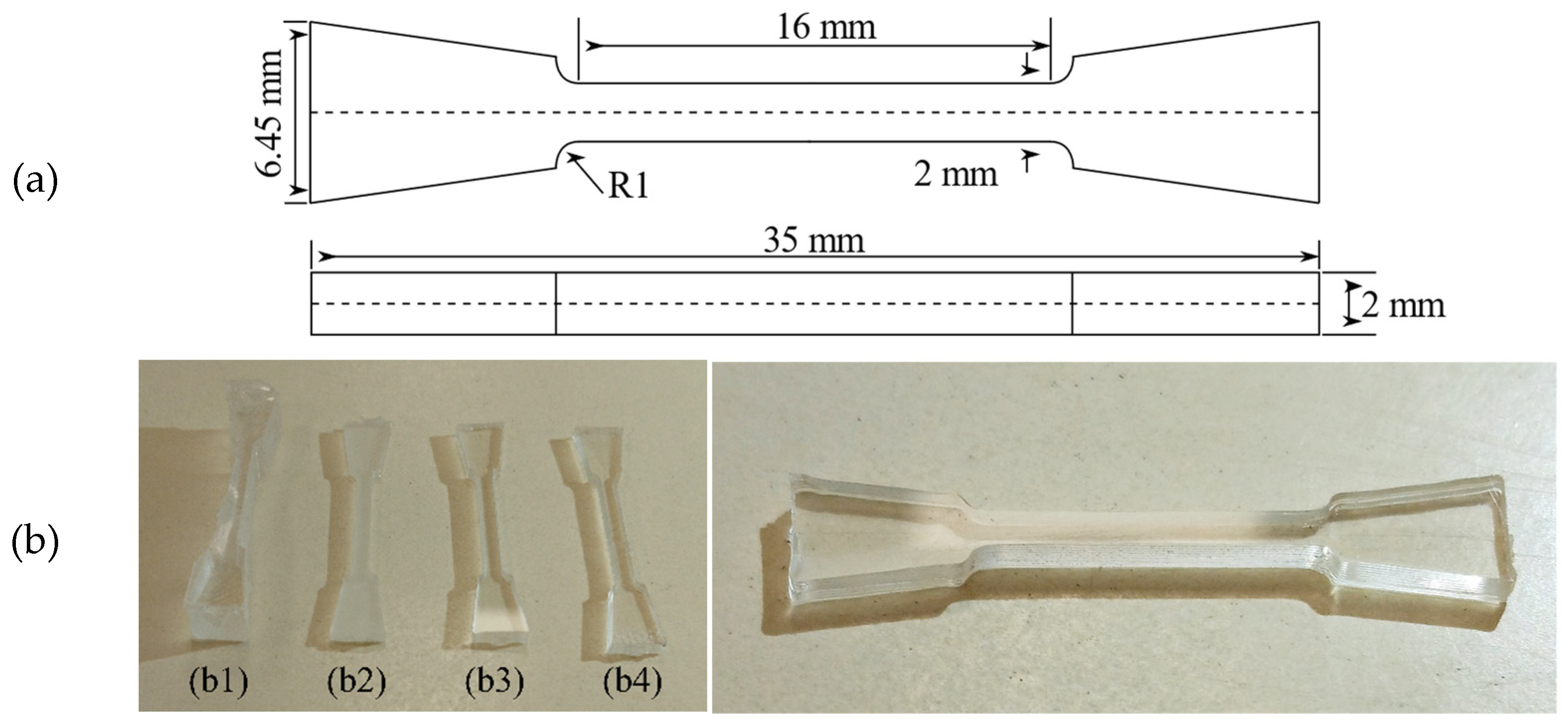
2.2. Specimen Preparation

In total, 37 samples were prepared, of which 35 were made with fiber. In addition, two samples without fiber were prepared to determine the experimental noise. The procedure for sample fabrication is detailed below.

The 35 fiber samples are prepared by extracting a single carbon fiber from the tow. The fiber is arranged in the center of the mold and then taped so that it retains constant tension. The resin is prepared according to the manufacturer’s recommendation in a 2:1 ratio. The prepared mixture is degassed by ultrasound for 10 min. The resin is then poured into the mold using a syringe so that no bubbles remain in the preparation. The curing time is 48 h at room temperature and then post-curing is carried out for 16 h at 70 °C in a muffle oven. The specimens are sanded symmetrically to a thickness of 2 mm and then polished to a mirror finish of 0.3 µm alumina grain size. The specimen geometry is shown in Figure 1a and the fabrication procedure is schematized in Figure 1b, where each stage up to the final mirror finish is shown. Analogous to the previous procedure, the two samples without fiber are prepared.

Before testing, the integrity of each sample is verified using a Nikon Optihot2 Pol polarized microscope (Nikon Instrument Inc., New York, NY, USA) with an objective lens 20×. A correct alignment of the fiber within the matrix and the presence of significant bubbles within the specimen is sought, discarding the samples that do not satisfy the standard.

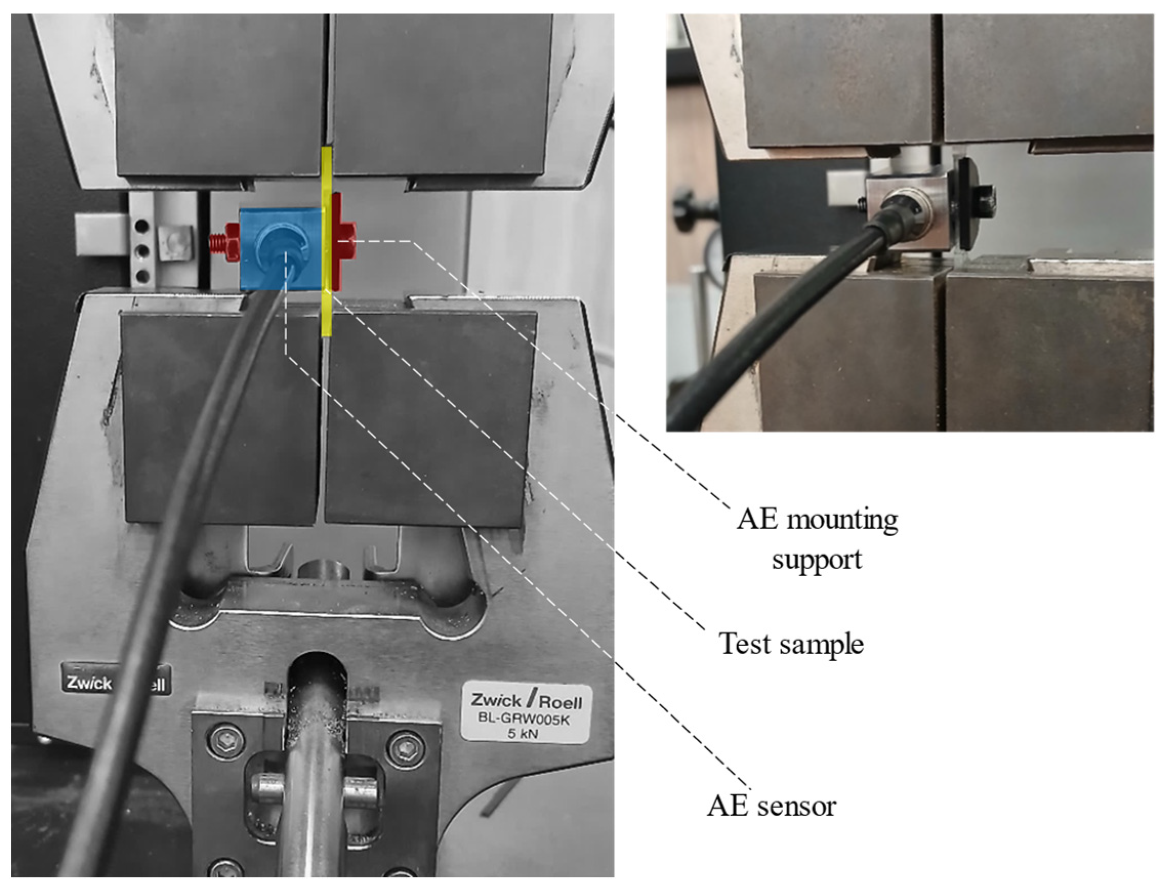
2.3. Experimental Setup

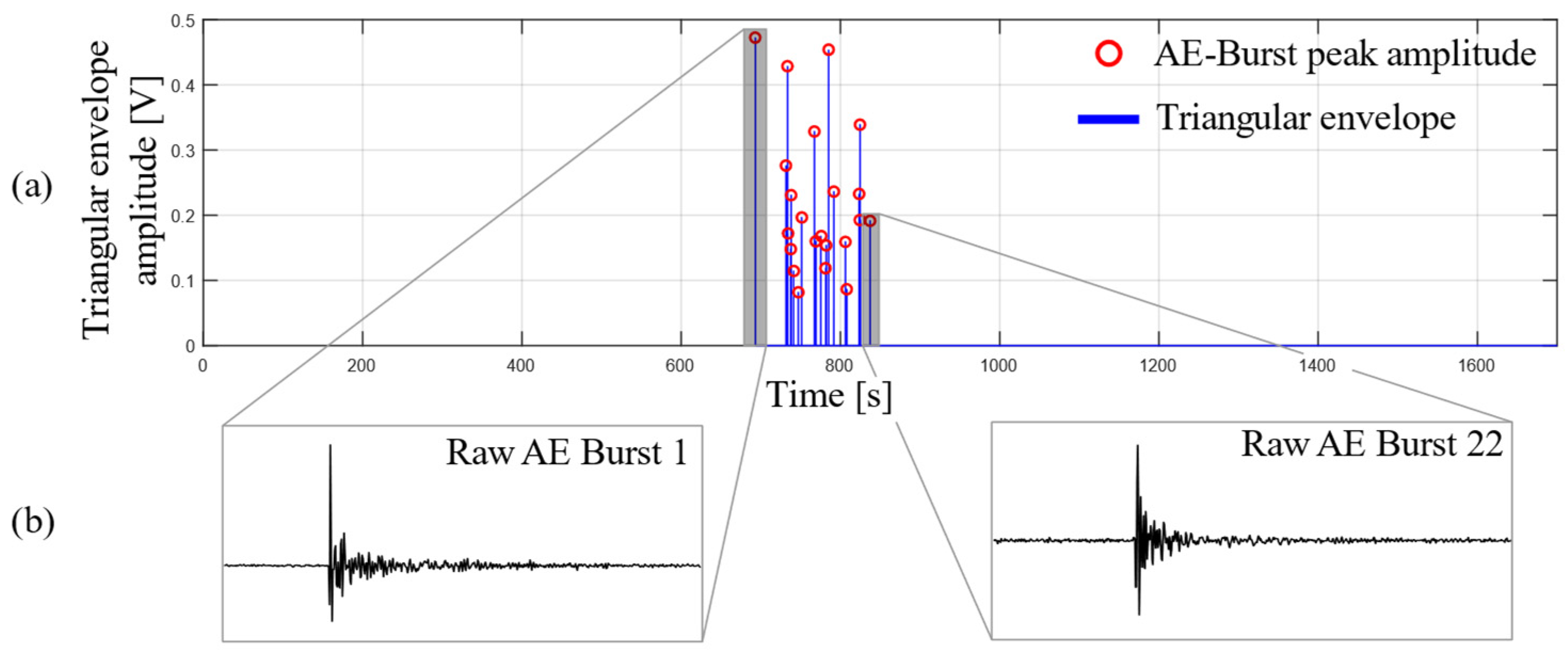
The tests are carried out on a Zwick Roell ProLine Z005 (ZwickRoell, Ulm, Germany) universal testing machine equipped with a 5 kN load cell, the test setup is shown in Figure 2. The test speed is 0.1 mm/min for approx. 20 min.

2.4. AE Measument

The AE measurement is performed using a Kistler 8152C (Kistler, Winterthur, Switzerland) broadband piezoelectric sensor, mounted directly in the center of the sample (see Figure 2). The sensor features a frequency range from 50 kHz to 900 kHz. A silicone grease couplant is used to facilitate the propagation of AE from the sample to the sensor. A Kistler 5125C (Kistler, Winterthur, Switzerland) pre-amplifier with an amplification factor of 10× is used. The amplified signal is acquired by a NI 9223 DAQ (National Instruments, Austin, TX, USA) at a sampling rate of 1 MHz. LabVIEW is used to control data acquisition and store the AE signals. Throughout the test, the raw AE signal is continuously measured for all samples.

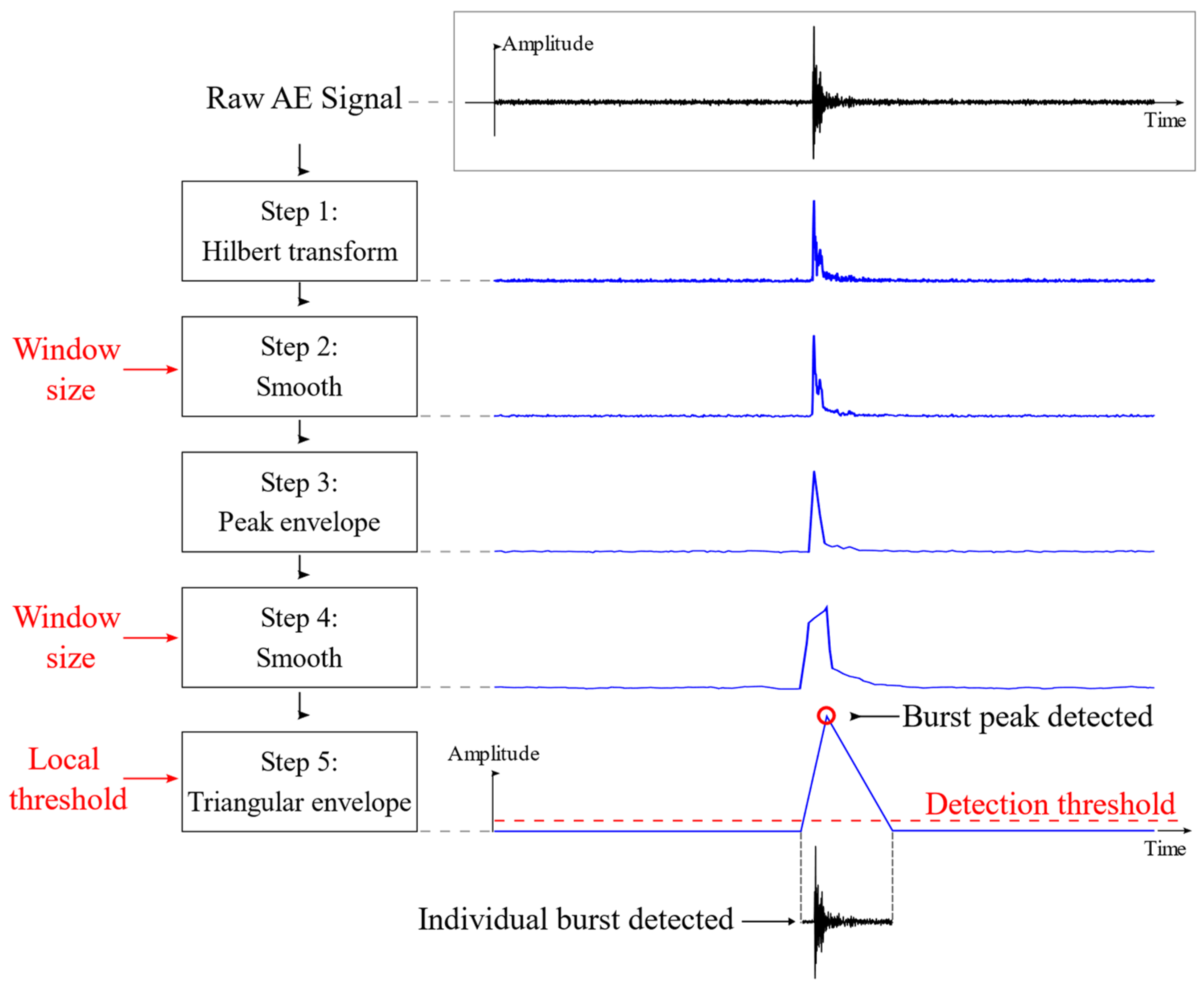
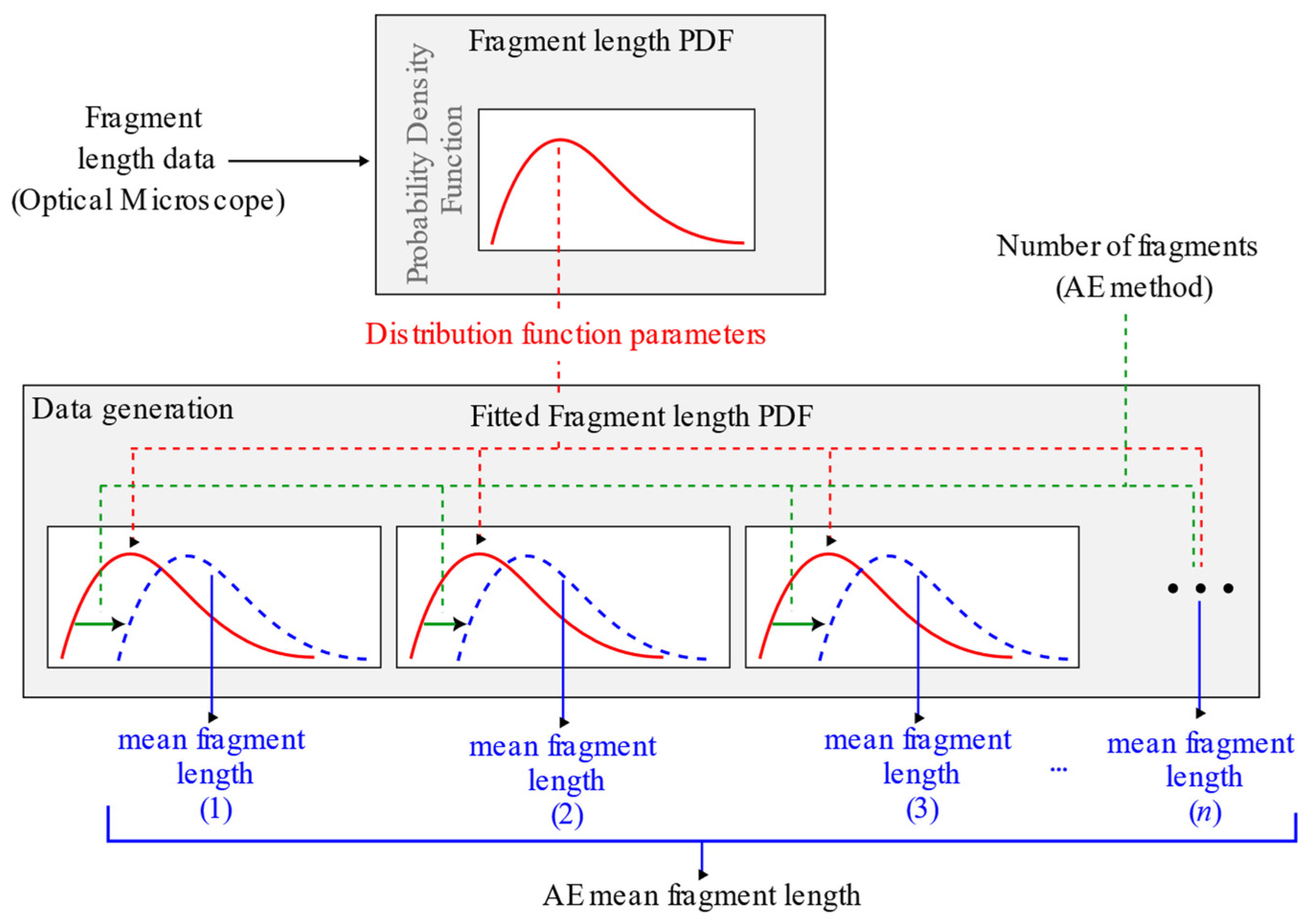
2.5. Fragment Count: AE Method

Fragment generation in the sample can be quantified by detecting bursts in the AE signal measured during tensile testing. The conventional approach for this purpose is the fixed threshold method; however, it presents significant limitations when applied to AE signals with a high density of bursts occurring within a short time window. When two or more bursts occur sufficiently close in time, they may be interpreted as a single, large event, resulting in the loss of information associated with individual events. Since fracture events do not follow any periodic pattern, it cannot be ensured that the bursts generated by fiber breakage will be sufficiently separated in time to be individually detected using the fixed threshold method. Unnthorsson [31] proposed a burst detection method designed to accurately identify events under such AE signal conditions. The core premise of this approach is the progressive simplification of the AE signal to obtain a triangular envelope, which enables the identification of individual bursts contained within the signal. The processed signal is generated by applying a series of processing steps, as shown in Figure 3.

• Step 1: An envelope of the raw AE signal is obtained by calculating the norm of the Hilbert transform on a logarithmic scale. This process reduces the difference between high and low-amplitude AE-bursts, thus enhancing their detectability.
• Step 2: A smoothing process is applied to reduce small fluctuations present in the signal obtained in Step 1. Smoothing is achieved by averaging the signal points using a moving window.
• Step 3: Eliminate all points in the signal obtained in the previous step that do not correspond to peaks. Since AE signals are measured at a high sampling rate, this process is performed twice to ensure the removal of non-relevant points for burst detection.
• Step 4: Apply a second smoothing using the same method as in Step 2.
• Step 5: The points of the signal that do not correspond to peaks or valleys are removed. Then, using a “local threshold” value, each point is compared with its neighborhood. If the amplitude difference between two neighboring points is smaller than the local threshold, the point with the smaller amplitude is removed, which helps to simplify the signal and improve the burst detection.

Step 5 is applied iteratively using progressively increasing values of the local threshold. The resulting signal from this process is an envelope composed of triangles, where each triangle with a peak amplitude exceeding a predefined detection threshold is identified as a burst. The start and end times of each triangle in the triangular envelope are obtained, and these values are used to extract the corresponding burst from the raw AE signal. Once the multiple AE-bursts have been identified, their number is counted for the IFSS calculation. The processing parameters of this method are the window size (Steps 2 and 4), the local threshold value (Step 5), and the detection threshold (Step 5). For burst detection in the AE signals measured during the tests of this study, a window size of 10 points is used. The local threshold is set at 35% of the maximum AE amplitude, and the detection threshold is defined as 0.005 V.

2.6. Fragment Measurement: Optical Microscope Method

A Nikon Optihot-2 polarizing microscope was used to measure the fragments at 10× magnification. To enhance fracture visualization, a 530 nm compensator was employed. Figure 4 presents representative images of the fragment features: Figure 4a illustrates a schematic of the debonding zone, where the central region represents the break gap, and the surrounding area indicates the sliding of the fiber relative to the matrix. Figure 4b, taken under unpolarized light at 20× magnification, provides a detailed view of the break. The low contrast between the fiber and the break gap can make fracturing complex and even impossible without the use of a polarizer in some cases. Also, note that the top image (Figure 4c) shows larger debonding areas compared to the bottom image (Figure 4d). For all samples, fragments were recorded along the calibrated reference length, with lengths ranging from 300 to 900 µm.

2.7. IFSS Calculation

The final calculation of the IFSS is carried out using the equations of Kelly and Tyson [22], but the procedure is slightly different for the two methods. Kelly and Tyson have shown that the value of the interfacial shear strength is calculated according to Equation (1):

$$IFSS={\displaystyle \frac{d{\sigma }_f}{2l_c}},$$

(1)

where $d$ denotes the fiber diameter, ${\sigma }_f$ is the fiber breaking strength and $l_c$ the critical fragment length which is considered according to [19] as a corrected length, see Equation (2):

$$l_c={\displaystyle \frac{4}{3}}{l}_{avg},$$

(2)

where $l_{avg}$ is the average length of the fragments.

Substituting (2) into (1) gives the final expression for calculating the IFSS:

$$IFSS={\displaystyle \frac{3}{8}}·{\displaystyle \frac{d{\sigma }_f}{l_{avg}}}.$$

(3)

2.7.1. Optical Microscope Method: Fragment Average Length

Optical measurements are performed for a set of specimens, which is considered the reference set. These measurements are then used to estimate the statistical distribution of the fragment lengths.

The set of fragment lengths measured using the optical microscope is denoted as $X$. The average fragment length using the optical microscope method is calculated using the arithmetic mean, see Equation (4):

$$l_{OP,avg}={\displaystyle \frac{\sum _{i=1}^{n_{OP,frag}}X\left(i\right)}{n_{OP,frag}}},$$

(4)

where $l_{OP,avg}$ is the average fragment length obtained by the optical method and $n_{OP,frag}$ is the number of fragments observed under the optical microscope.

2.7.2. AE Method: Fragment Average Length

The calculation used to obtain the average fragment length using the AE method is based on the probability density function derived from the optical measurements described in the previous subsection. This probability function determines which statistical distribution best fits the measured data. To this end, Q-Q (quantile–quantile) plots were employed to visually compare the empirical data distribution against various theoretical models. Specifically, the fragment length data were compared to Weibull, Lognormal, Exponential, Gamma, and Gaussian distributions. The Q-Q plots help assess the goodness-of-fit by displaying how closely the data quantiles align with those of a given theoretical distribution. Deviations from the reference line indicate discrepancies, allowing for a qualitative assessment prior to any statistical testing.

A Gamma distribution was selected in this case, as the observed fragment length data exhibit a clear positive skew. Additionally, the Kolmogorov–Smirnov (K-S) test was used to validate each distribution’s fit quantitatively. The Gamma distribution yielded the lowest K-S statistic among the tested models, confirming its suitability for representing the probability density of the fragment lengths. The probability density function used is shown in Equation (5):

$$f\left(x_i;k,\theta \right)={\displaystyle \frac{x^{k-1}{e}^{-\frac{x_i}{\theta }}}{{\theta }^k\Gamma \left(k\right)}},$$

(5)

where $k$ is the shape parameter, $\theta$ is the scale parameter, $x_i$ is the value at which the gamma distribution will be evaluated, and $\Gamma$ is the gamma function.

To fit the gamma distribution to the values of the fragment lengths $X$, the negative log-likelihood function of the gamma distribution is minimized, see Equation (6),

$$\mathcal{l}\left(k,\theta \right)=\left(k-1\right)\sum _{i=1}^m\ln \left(X_i\right)-{\displaystyle \frac{1}{\theta }}\sum _{i=1}^m{X}_i-m·k·ln\left(\theta \right)-m·\ln \left(\Gamma \left(k\right)\right),$$

(6)

where $\mathcal{l}(k,\theta )$ is the negative of the log-likelihood of the gamma distribution, $m$ is the number of fragments in a sample, $X_i$ is the i-th fragment length in a sample.

The result of minimizing Equation (6) gives the parameters $k$ and $\theta$ of the gamma distribution that best fits the fragment length data measured with the microscope. The obtained gamma distribution will be used to correct the length of the fragments detected with the AE method.

In the AE method, bursts are detected, which represents the release of a sufficiently large amount of energy to be detected by the sensor. Therefore, it is assumed that the occurrence of one of these events is due to the formation of a crack in the fiber, i.e., when two AE events occur, it implies that the fiber was broken into a single fragment within the calibrated zone. Consequently, the number of fragments as a function of AE events is shown in Equation (7):

$$n_{AE,frag}=n_{AE,burst}-1,$$

(7)

where $n_{AE,frag}$ is the number of fragments counted using the AE method, and $n_{AE,burst}$ is the number of AE-bursts detected in the AE signal.

The next step is to correct the previously obtained gamma distribution. This is based on the number of fragments detected using the AE method $n_{AE,frag}$, since the fragment length is directly dependent on their quantity. As the number of fragments increases, the average length decreases, causing the distribution to shift to the left. On the other hand, if the number of fragments decreases, the distribution shifts to the right.

To correct the gamma distribution according to the number of fragments, a set of data points is generated from the previously obtained distribution, equal to the number of fragments $n_{AE,frag}$. Once obtained, the data are rescaled so that their sum equals the total fragmented length of the samples, as shown in Equation (8):

$$l_{total\_frag}=F·\sum _{i=1}^{n_{AE,frag}}{X}^{\prime }\left(i\right),$$

(8)

where $l_{total\_frag}$ represents the sum of the lengths of all fragments within the sample, $X^{\prime }$ are the fragment lengths generated by the gamma distribution, and $F$ is the rescaling factor.

Therefore, the rescaled data are calculated according to Equation (9):

$$X_{scaled}=F·X\prime ,$$

(9)

where $X_{scaled}$ are the rescaled generated data.

The process of data generation and rescaling is performed $n_{gen}$ times. For each data generation, the parameters $k$ and $\theta$ of the fitted gamma distribution are obtained, which are then used to calculate the average fragment length obtained in the $j$-th data generation, see Equation (10):

$$l_{AE,avg,j}=k_j·{\theta }_j,$$

(10)

where $l_{AE,avg,j}$ is the average fragment length for the data generated at the $j$-th iteration, which is calculated using the parameters of the fitted gamma distribution, $k_j$ is the shape parameter in the $j$-th iteration; ${\theta }_j$ is the scale parameter in the $j$-th iteration.

The average fragment length that will be used in the IFSS calculation is obtained by averaging the results from all iterations, see Equation (11):

$$l_{AE,avg,fitted}=\sum _{j=1}^{n_{gen}}{\displaystyle \frac{l_{AE,avg,j}}{n_{gen}}},$$

(11)

where $l_{AE,avg,fitted}$ is the average fragment length obtained from the fitted gamma distribution in the AE method. Figure 5 shows a graphical summary of the procedure described above.

The IFSS is calculated using the results provided by the model $l_{AE,avg,fitted}$. In parallel, to compare the results, the average fragment length is calculated using the calibrated length of the samples, as shown in Equation (12):

$$l_{AE,avg,arithmetic}={\displaystyle \frac{l_{cal}}{n_{AE,frag}}},$$

(12)

where $l_{AE,avg,arithmetic}$ is the average fragment length calculated using the arithmetic mean, $l_{cal}$ is the calibrated length of the sample, and $n_{AE,frag}$ is the number of fragments calculated using the AE method.

2.7.3. Calculation Error

To compare the obtained results, the error of the IFSS from the AE method is calculated with respect to the optical microscope method for each of the samples, see Equation (13):

$${IFSS}_{error,i}=100·{\displaystyle \frac{abs\left({IFSS}_{OP,i}-{IFSS}_{AE,i}\right)}{{IFSS}_{OP,i}}},$$

(13)

where ${IFSS}_{error,i}$ is the error on the IFSS for the $i$-th sample, ${IFSS}_{OP,i}$ is the value obtained using the optical microscope method for the $i$-th sample, and ${IFSS}_{AE,i}$ is the value obtained with the AE method.

3. Results and Discussion

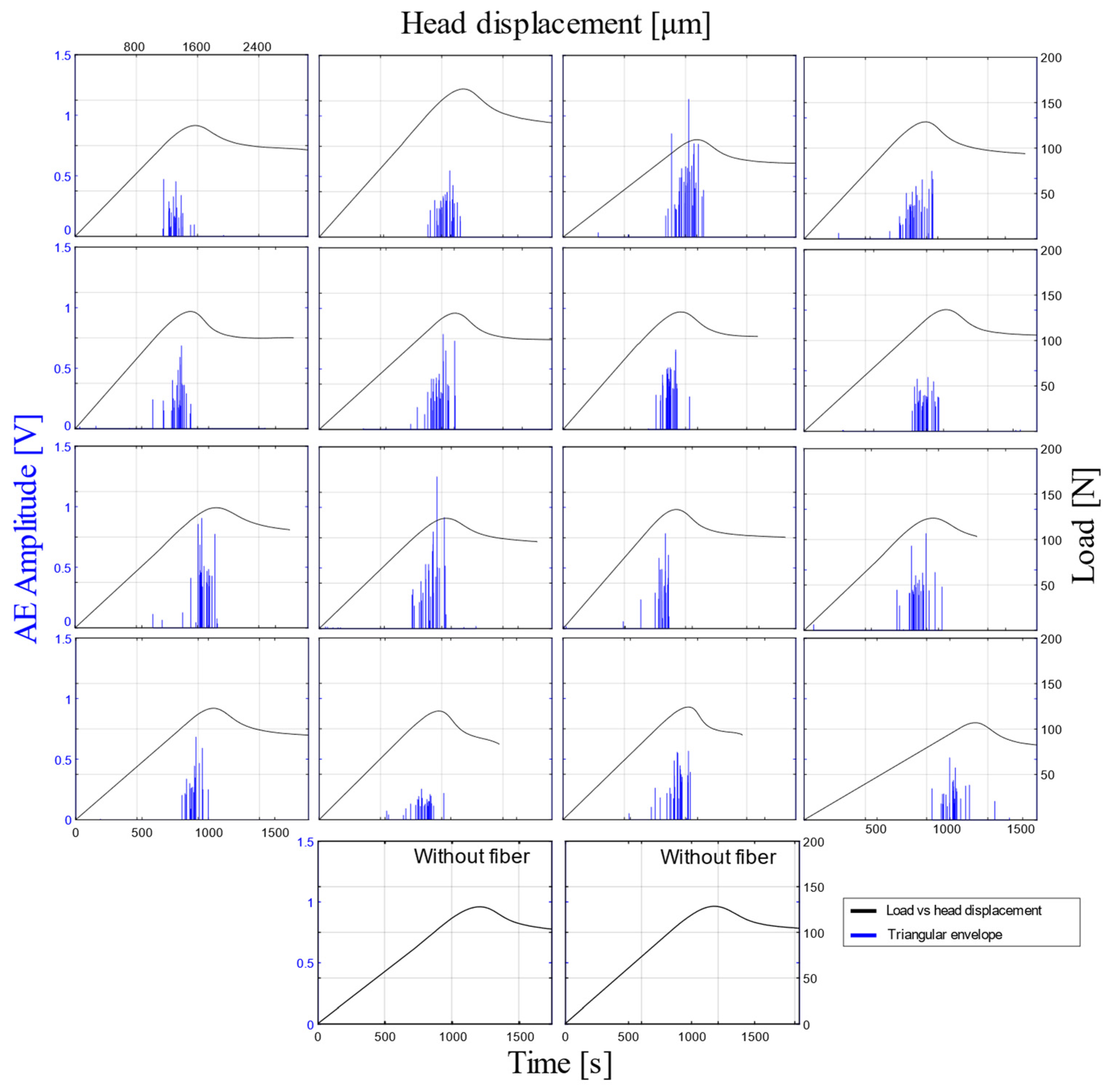
3.1. Acoustic Emission Data

Thirty-five SFFTs were performed to determine the IFSS using optical and AE methods to obtain the length of the fragments. Figure 6 shows the result of the burst detection process applied to the AE signal measured during one of the tests. In Figure 6a, the triangular envelope is shown, which is composed of individual triangles representing the occurrence of AE-bursts. It is important to note that, due to the very short duration of the bursts relative to the total signal length, the triangles in the envelope appear as vertical lines. Figure 6b provides a detailed view of the AE-bursts corresponding to two of the triangles in the envelope. The duration of the tests performed is approximately 20 min, and the time range in which most bursts occur spans around 4 min. Additionally, the average number of AE bursts detected in the tests generally does not exceed 30. This indicates a low temporal density of bursts, meaning that in this type of signal, the conventional fixed threshold method should have no difficulty detecting them. Moreover, the bursts observed in the AE signals (see Figure 6b) exhibit a well-defined shape, which facilitates their detection. The AE waveforms observed in [25,27] are similar to those obtained in this study.

Figure 7 shows the triangular envelopes obtained during the burst detection process from AE signals, as well as the (load vs. head displacement) curves obtained during the tests of 16 SFFT samples and the two specimens without fiber. The results indicate the absence of AE burst activity in the samples without fiber, confirming that AE bursts originate from internal failures within the specimen, primarily due to fiber fragmentation. A comparison between the number of AE events and the fragment counts obtained through optical measurements reveals a systematic discrepancy: in most tests, AE detects more fragments than the number identified optically. This apparent overestimation contrasts with the findings of Feih et al. [32], who reported that energy dissipation within the matrix could lead to the loss of AE events. A possible explanation for this discrepancy is the improved sensitivity and resolution of modern AE sensors, which may now be capable of capturing a greater number of localized failure events.

3.2. Fiber Fragmentation Characterization

After each test, the fragments were measured microscopically and observed in the calibrated area of the sample. The fragments were generally located within a few micrometers of the calibrated length, and no fractures were observed outside the study area. This procedure allowed the direct determination of reference fragment lengths for each sample.

In Figure 7, it is observed that the AE events are mainly concentrated before the plastic regime of the material, a similar behavior is observed in [25,26,33]. This occurs because the first stage of the test begins when the load transferred from the matrix to the fiber exceeds its tensile strength. When the plastic regime is reached, the creep of the specimen prevents the matrix from sustaining additional stress, reducing the transferred stress to the fiber and preventing the generation of new fragments [34].

In optical measurement, carbon fiber can cause confusion due to the low contrast it presents relative to the failure zones. Polarized light facilitates observation thanks to the birefringence generated by the stress field in the resin surrounding the fiber. At the interface, qualitative patterns can be identified as indicating the level of adhesion. The observed evidence of an extended detachment region, where relative fiber slippage occurs, is referred to as a debond zone, partially generated by the rupture of molecular bonds within the interphase [33]. Previous studies have reported this phenomenon in unloaded samples with particularly weak interfaces, such as carbon fiber with epoxy resin [16,19]. These findings align with fragment lengths ranging from 300 µm to 900 µm, and these ranges have also been observed in unsized carbon fibers [35].

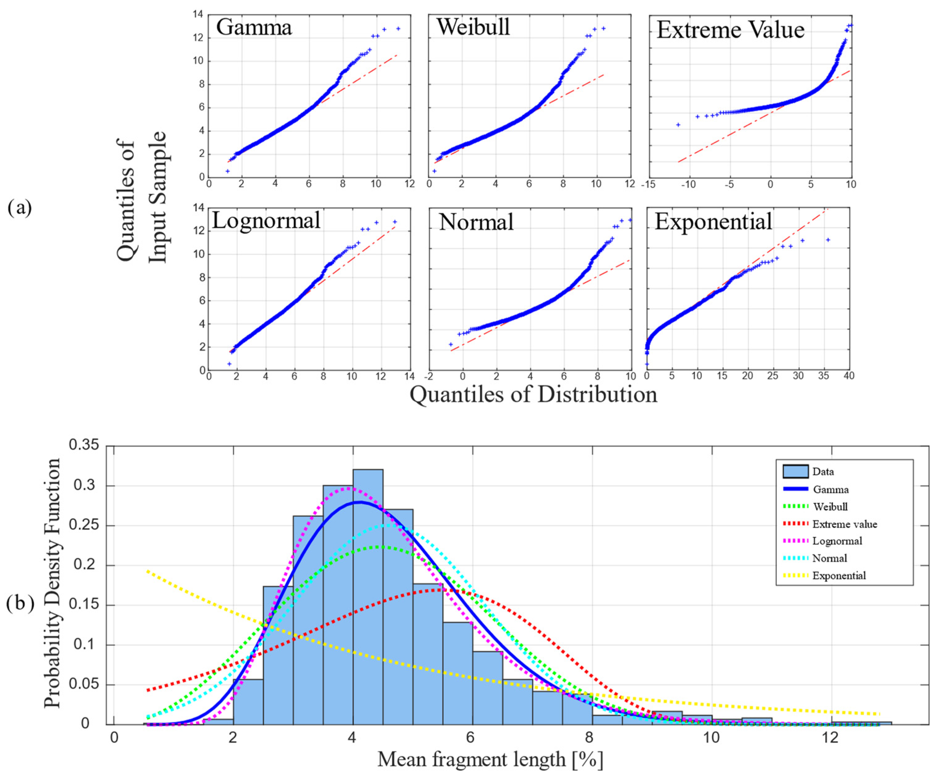
3.3. Statistical Analysis of Fragment Distribution

Figure 8a displays the Q-Q plots, which demonstrate the expected linear behavior for both the Gamma and Lognormal distributions. This indicates a strong alignment between the empirical data and these theoretical models. In both cases, the data points closely follow the reference line across most of the distribution range, especially in the central quantiles. This suggests that these distributions effectively capture the shape and skewness of the measured fragment length data, see Figure 8b. Minor deviations at the tails are anticipated due to the limited number of extreme values. Although the Weibull distribution is commonly reported in the literature for modeling fragment lengths [28,35], it did not provide the best fit for the data in this study. The superior performance of the Gamma and Lognormal distributions in the Q-Q plots suggests that these models more accurately represent the observed behavior. Nonetheless, it is important to note that both Gamma and Weibull distributions share key characteristics—such as being defined over positive values and exhibiting positive skewness—which supports the use of Gamma as a valid alternative. The Kolmogorov–Smirnov test supports the observations from the Q-Q plot, revealing that the Gamma and Lognormal distributions have the lowest statistics, at $4.7·{10}^{-4}$ and $7.2·{10}^{-3}$, respectively. The Gamma distribution was ultimately chosen because it strikes a balance between statistical performance and practical applicability in the context of material mechanics, while also minimizing the risk of model overfitting.

Table 1. Mean fragment lengths obtained using the AE method with different methodologies: arithmetic mean and fitted distribution curve.

Number of Fragments	AE Method Mean Fragment Length [%]		Number of Fragments	AE Method Mean Fragment Length [%]
	Arithmetic Mean	Fitted Distribution		Arithmetic Mean	Fitted Distribution
1	100.00	100.00	21	4.76	3.41
2	50.00	35.81	22	4.55	3.24
3	33.33	23.84	23	4.35	3.10
4	25.00	17.91	24	4.17	2.98
5	20.00	14.31	25	4.00	2.86
6	16.67	11.91	26	3.85	2.75
7	14.29	10.19	27	3.70	2.65
8	12.50	8.93	28	3.57	2.55
9	11.11	7.94	29	3.45	2.47
10	10.00	7.13	30	3.33	2.38
11	9.09	6.49	31	3.23	2.30
12	8.33	5.98	32	3.13	2.23
13	7.69	5.49	33	3.03	2.17
14	7.14	5.09	34	2.94	2.10
15	6.67	4.76	35	2.86	2.05
16	6.25	4.47	36	2.78	1.99
17	5.88	4.20	37	2.70	1.93
18	5.56	3.96	38	2.63	1.88
19	5.26	3.76	39	2.56	1.83
20	5.00	3.58	40	2.50	1.79

shows the averages of the fragment lengths used in the AE method, calculated using the following two approaches: the arithmetic mean and the fitted gamma distribution proposed method. It can be observed that the average estimated with this method is lower than that obtained with the arithmetic mean.

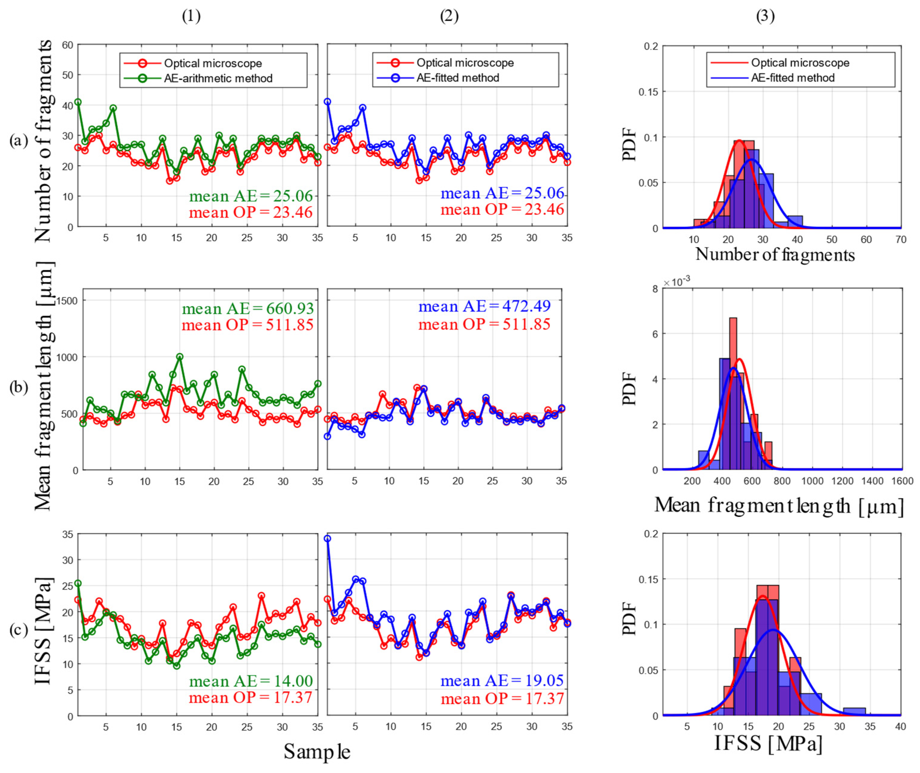
3.4. Comparison of AE and Optical Microscopy Methods

Figure 9 shows the number of fragments, average lengths, and IFSS values for the specimens tested with both methods. Figure 9(a1,b1,c1) presents the results obtained by the AE method using $l_{AE,avg,arithmetic}$ and the optical microscope method using $l_{OP,avg}$. Figure 9(a2,b2,c2) also compares both methods, but in this case, the AE method $l_{AE,avg,fitted}$ is used. Finally, Figure 9(a3,b3,c3) presents the normal distributions corresponding to the results shown in Figure 9(a2,b2,c2). It is important to note that the number of fragments shown in Figure 9(a1,a2) is the same.

Figure 9(a1,a2) reveal that the average number of fragments detected with the AE method is 6.82% higher than that obtained with the conventional optical microscopy method, suggesting that the AE sensor detects events caused by phenomena other than fiber fragmentation, such as slippage of the fiber–matrix interface.

To determine whether the detected AE-bursts are caused by one or the other phenomenon, conventional indicators were calculated. However, since the tests performed were not focused on characterizing the different types of failure in this type of material, the results obtained were not conclusive for the present investigation but present an interesting topic for future research.

Figure 9(b1,b2) show the mean fragment length obtained with both methods. It can be observed that, for the data as a whole, the AE-arithmetic method overestimates the value by 29.13% concerning the optical method. This is because this methodology assumes a uniform distribution in the fragments, ignoring the real variability in their length. On the other hand, the AE-fitted method offers a more precise estimate, reducing the average difference to 7.69%.

Figure 9(c1,c2) show the results of the IFSS calculation for both methods. Since the AE arithmetic method overestimates the fragment length and considers the equation used to calculate the IFSS, this method underestimates the total values by 19.40% concerning the optical method. On the other hand, the AE-fitted method gives results with a difference of 9.67% compared to the optical method.

The absolute error of the IFSS obtained by the AE method concerning the optical method is calculated for each sample tested, according to Equation (13), to analyze the results of each sample separately. The average individual error in the calculation of the IFSS with the AE arithmetic method is 22.36% compared to the optical method, while the AE-fitted method has an error of 10.42%. The confidence intervals are shown in

Table 2. Confidence intervals for the IFSS error of the AE method compared to the optical microscopy method. The two methodologies used to calculate the average fragment lengths in the AE method are analyzed: arithmetic mean and fitted distribution.

		IFSS Error [%]
		AE-Fitted Method	AE-Arithmetic Method
Mean Individual Error		10.42	22.36
Confidence interval	50%	10.52	22.57
	75%	11.80	25.32
	95%	14.16	30.37

, where it is observed that with the AE-fitted method, 95% of the samples have a maximum error of 14.16%. In contrast, for the same confidence level, the AE arithmetic method has a maximum error of 30.37%. In the AE-arithmetic method, the predominant source of error is due to the estimation of the average fragment length. In contrast, the error associated with the fitted AE method is significantly lower, as the developed model aims to compensate for this inaccuracy by incorporating the fragment data observed under the microscope. The error related to the estimation of the number of fragments is common to both the AE-arithmetic and AE-fitted methods; therefore, it does not affect the comparative evaluation between them. The error in the AE-fitted method primarily stems from the uncertainty in detecting the number of fragments and from the residual error associated with the use of the developed model. Since these errors are comparatively smaller than the error in the estimation of the average fragment length, the overall error of the AE-fitted method is lower in comparison to the AE-arithmetic method.

4. Conclusions

This article presents a method for calculating the interfacial shear strength in single-fiber fragmentation tests using acoustic emission techniques combined with statistical distribution fitting. Based on the results, the conclusions are drawn as follows:

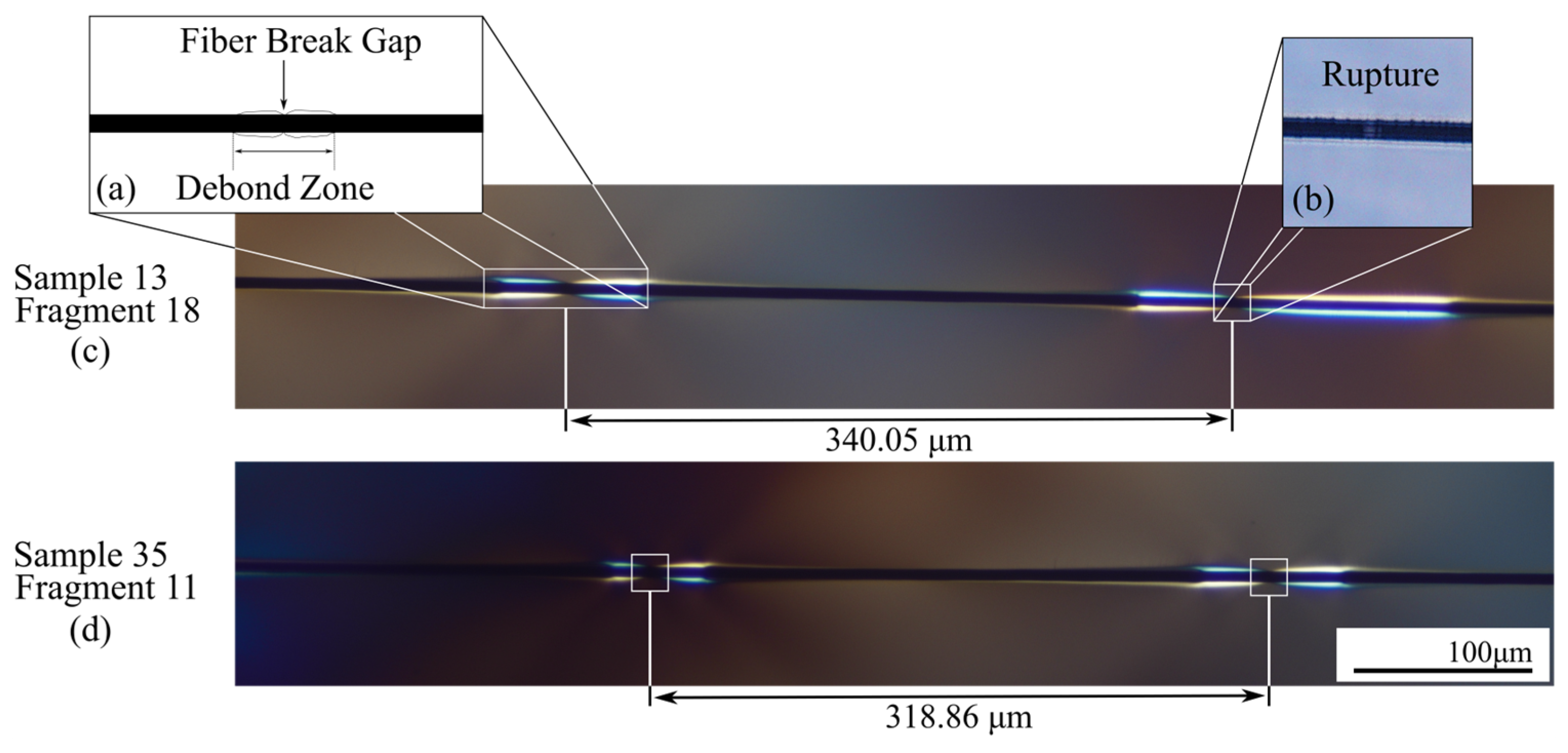
• Specimens manufactured without fiber do not exhibit AE activity in their signals. Therefore, the presence of bursts in the AE signals measured during the SFFTs is related to the fiber failure mechanisms inside the specimens.
• The fragment lengths observed in the specimens after the SFFTs follow a distribution with a positive skew. Therefore, the distributions that best fit the data are the lognormal and gamma distributions.
• A methodology is developed to estimate the average fragment length using a fitted gamma distribution based on the number of fragments measured with the AE method. The values obtained from this distribution allow the incorporation of the positive skew observed in the fragment lengths into the calculation of IFSS using AE.
• The IFSS error from the AE-arithmetic method, compared to the optical microscope method, is 30.37% at a 95% confidence level. On the other hand, the error from the AE-fitted method is 14.16% at a 95% confidence level. The AE-fitted method provides significantly better results than the AE-arithmetic method, as it considers the distribution of fragment lengths experimentally observed in the SFFTs.
• A potential source of error lies in the mounting of the AE sensor, where a mounting support is used to press the sensor against the specimen to facilitate AE detection and prevent slippage between the two elements. However, as the specimen deforms and its cross-sectional area reduces, the pressure of the support also decreases, which could cause movements detected by the sensor and introduce an error in the IFSS calculation.

The main advantages of the AE-fitted method compared to the optical method are the elimination of the labor hours required for fragment counting and measurement under the optical microscope, as well as its ease of application in composite materials with opaque matrices and interfaces with high adhesion.

To advance the understanding and characterization of interfacial properties in micromechanical testing of composite materials through acoustic emissions, the following research lines are proposed:

• Use of multiple AE sensors: Implementing two or more AE sensors on the specimen allows locating events within the specimen through triangulation and thus estimating the length of the generated fragments. This approach could be evaluated in combination with different specimen geometries, considering the influence of sensor position on the quality of the detected signals.
• Influence of IFSS on the measured AE signal: The objective is to analyze how different adhesion levels affect the generation and burst detection. It could be evaluated whether a higher IFSS alters the AE indicators of the detected bursts, as stronger interfaces could generate different signals due to higher energy accumulation before rupture.

References

1. Liu, L.; Jia, C.; He, J.; Zhao, F.; Fan, D.; Xing, L.; Wang, M.; Wang, F.; Jiang, Z.; Huang, Y. Interfacial characterization, control and modification of carbon fiber reinforced polymer composites. Compos. Sci. Technol. 2015, 121, 56–72. [Google Scholar] [CrossRef]
2. Yao, T.T.; Wu, G.P.; Song, C. Interfacial adhesion properties of carbon fiber/polycarbonate composites by using a single-filament fragmentation test. Compos. Sci. Technol. 2017, 149, 108–115. [Google Scholar] [CrossRef]
3. Zhou, J.; Li, Y.; Li, N.; Hao, X.; Liu, C. Interfacial shear strength of microwave processed carbon fiber/epoxy composites characterized by an improved fiber-bundle pull-out test. Compos. Sci. Technol. 2016, 133, 173–183. [Google Scholar] [CrossRef]
4. Zheng, H.; Zhang, W.; Li, B.; Zhu, J.; Wang, C.; Song, G.; Wu, G.; Yang, X.; Huang, Y.; Ma, L. Recent advances of interphases in carbon fiber-reinforced polymer composites: A review. Compos. Part B Eng. 2022, 233, 109639. [Google Scholar] [CrossRef]
5. Kim, J.K.; Mai, Y.W. (Eds.) Engineered Interfaces in Fiber Reinforced Composites; Elsevier: Amsterdam, The Netherlands, 1998. [Google Scholar]
6. Lin, J.; Sun, C.; Min, J.; Wan, H.; Wang, S. Effect of atmospheric pressure plasma treatment on surface physicochemical properties of carbon fiber reinforced polymer and its interfacial bonding strength with adhesive. Compos. Part B Eng. 2020, 199, 108237. [Google Scholar] [CrossRef]
7. Yokozeki, T.; Ishibashi, M.; Kobayashi, Y.; Shamoto, H.; Iwahori, Y. Evaluation of adhesively bonded joint strength of CFRP with laser treatment. Adv. Compos. Mater. 2016, 25, 317–327. [Google Scholar] [CrossRef]
8. Stojcevski, F.; Hilditch, T.B.; Henderson, L.C. A comparison of interfacial testing methods and sensitivities to carbon fiber surface treatment conditions. Compos. Part A Appl. Sci. Manuf. 2019, 118, 293–301. [Google Scholar] [CrossRef]
9. Yuan, H.; Zhang, S.; Lu, C.; He, S.; An, F. Improved interfacial adhesion in carbon fiber/polyether sulfone composites through an organic solvent-free polyamic acid sizing. Appl. Surf. Sci. 2013, 279, 279–284. [Google Scholar] [CrossRef]
10. Wang, C.; Xia, L.; Zhong, B.; Yang, H.; Huang, L.; Xiong, L.; Huang, X.; Wen, G. Fabrication and mechanical properties of carbon fibers/lithium aluminosilicate ceramic matrix composites reinforced by in-situ growth SiC nanowires. J. Eur. Ceram. Soc. 2019, 39, 4625–4633. [Google Scholar] [CrossRef]
11. Liu, Y.T.; Song, H.Y.; Yao, T.T.; Zhang, W.S.; Zhu, H.; Wu, G.P. Effects of carbon nanotube length on interfacial properties of carbon fiber reinforced thermoplastic composites. J. Mater. Sci. 2020, 55, 15467–15480. [Google Scholar] [CrossRef]
12. Feng, P.; Song, G.; Li, X.; Xu, H.; Xu, L.; Lv, D.; Zhu, X.; Huang, Y.; Ma, L. Effects of different “rigid-flexible” structures of carbon fibers surface on the interfacial microstructure and mechanical properties of carbon fiber/epoxy resin composites. J. Colloid Interface Sci. 2021, 583, 13–23. [Google Scholar] [CrossRef] [PubMed]
13. Tian, Y.; Zhang, H.; Zhang, Z. Influence of nanoparticles on the interfacial properties of fiber-reinforced-epoxy composites. Compos. Part A Appl. Sci. Manuf. 2017, 98, 1–8. [Google Scholar] [CrossRef]
14. Yi, M.; Sun, H.; Zhang, H.; Deng, X.; Cai, Q.; Yang, X. Flexible fiber-reinforced composites with improved interfacial adhesion by mussel-inspired polydopamine and poly (methyl methacrylate) coating. Mater. Sci. Eng. C 2016, 58, 742–749. [Google Scholar] [CrossRef] [PubMed]
15. Brunner, A.J.; Schwiedrzik, J.J.; Mohanty, G.; Michler, J. Fiber push-in failure in carbon fiber epoxy composites. Procedia Struct. Integr. 2020, 28, 538–545. [Google Scholar] [CrossRef]
16. Nikforooz, M.; Verschatse, O.; Daelemans, L.; De Clerck, K.; Van Paepegem, W. Mixed experimental-numerical method for quantitative measurement of mode II fibre/matrix interface debonding and comparison of fibre sizings in single short fibre composites. Polym. Test. 2024, 134, 108435. [Google Scholar] [CrossRef]
17. Stojcevski, F.; Hilditch, T.B.; Gengenbach, T.R.; Henderson, L.C. Effect of carbon fiber oxidization parameters and sizing deposition levels on the fiber-matrix interfacial shear strength. Compos. Part A Appl. Sci. Manuf. 2018, 114, 212–224. [Google Scholar] [CrossRef]
18. Tominaga, Y.; Shimamoto, D.; Hotta, Y. Quantitative evaluation of interfacial adhesion between fiber and resin in carbon fiber/epoxy composite cured by semiconductor microwave device. Compos. Interfaces 2016, 23, 395–404. [Google Scholar] [CrossRef]
19. Ahmadvash Aghbash, S.; Verpoest, I.; Swolfs, Y.; Mehdikhani, M. Methods and models for fibre–matrix interface characterisation in fibre-reinforced polymers: A review. Int. Mater. Rev. 2023, 68, 1245–1319. [Google Scholar] [CrossRef]
20. Qi, G.; Zhang, B.; Yu, Y. Research on carbon fiber/epoxy interfacial bonding characterization of transverse fiber bundle composites fabricated by different preparation processes: Effect of fiber volume fraction. Polym. Test. 2016, 52, 150–156. [Google Scholar] [CrossRef]
21. Stojcevski, F.; Hilditch, T.; Henderson, L.C. A modern account of Iosipescu testing. Compos. Part A Appl. Sci. Manuf. 2018, 107, 545–554. [Google Scholar] [CrossRef]
22. Kelly, A.; Tyson, A.W. Tensile properties of fibre-reinforced metals: Copper/tungsten and copper/molybdenum. J. Mech. Phys. Solids 1965, 13, 329–350. [Google Scholar] [CrossRef]
23. Batista, M.D.R.; Drzal, L.T. Carbon fiber/epoxy matrix composite interphases modified with cellulose nanocrystals. Compos. Sci. Technol. 2018, 164, 274–281. [Google Scholar] [CrossRef]
24. Liu, Y.T.; Li, L.; Wang, J.P.; Fei, Y.J.; Liu, N.D.; Wu, G.P. Effect of carbon nanotube addition in two sizing agents on interfacial properties of carbon fiber/polycarbonate composites. New Carbon Mater. 2021, 36, 639–648. [Google Scholar] [CrossRef]
25. Hamam, Z.; Godin, N.; Fusco, C.; Monnier, T. Modelling of fiber break as Acoustic Emission Source in Single Fiber Fragmentation Test: Comparison with experimental results. J. Acoust. Emiss. 2018, 35, 1–12. [Google Scholar]
26. Nordstrom, R.A. Acoustic Emission Characterization of Microstructural Failure in the Single Fiber Fragmentation Test (No. 235); EMPA: Dübendorf, Switzerland, 1996. [Google Scholar]
27. Park, J.M.; Kong, J.W.; Kim, J.W.; Yoon, D.J. Interfacial evaluation of electrodeposited single carbon fiber/epoxy composites by fiber fracture source location using fragmentation test and acoustic emission. Compos. Sci. Technol. 2004, 64, 983–999. [Google Scholar] [CrossRef]
28. Drzal, L.T.; Rich, M.J.; Camping, J.D.; Park, W.J. Interfacial shear strength and failure mechanisms in graphite fiber composites. In Proceedings of the 35th Annual Technical Conference Reinforced Plastics; Composites Institute, The Society of the Plastics Industry, Inc.: New Orleans, LA, USA, 1980. [Google Scholar]
29. Moradian, Z.; Li, B. Hit-Based Acoustic Emission Monitoring of Rock Fractures: Challenges and Solutions; Springer: Cham, Switzerland, 2017. [Google Scholar] [CrossRef]
30. Leaman, F.; Niedringhaus, C.; Hinderer, S.; Nienhaus, K. Evaluation of acoustic emission burst detection methods in a gearbox under different operating conditions. J. Vib. Control 2018, 25, 895–906. [Google Scholar] [CrossRef]
31. Unnthorsson, R. Hit Detection and Determination in AE Bursts; IntechOpen: London, UK, 2013. [Google Scholar] [CrossRef]
32. Feih, S.; Wonsyld, K.; Minzari, D.; Westermann, P.; Lilholt, H. Testing Procedure for the Single Fiber Fragmentation Test; Risø National Laboratory: Roskilde, Denmark, 2004. [Google Scholar]
33. Kim, B.W.; Nairn, J.A. Observations of fiber fracture and interfacial debonding phenomena using the fragmentation test in single fiber composites. J. Compos. Mater. 2002, 36, 1825–1858. [Google Scholar] [CrossRef]
34. Vautey, P.; Favre, J.P. Fibre/matrix load transfer in thermoset and thermoplastic composites—Single fibre models and hole sensitivity of laminates. Compos. Sci. Technol. 1990, 38, 271–288. [Google Scholar] [CrossRef]
35. Liu, F.; Shi, Z.; Dong, Y. Improved wettability and interfacial adhesion in carbon fibre/epoxy composites via an aqueous epoxy sizing agent. Compos. Part A Appl. Sci. Manuf. 2018, 112, 337–345. [Google Scholar] [CrossRef]
Figure 1. (a) Sample geometry, (b) Stages of the preparation (b1) sample out of mold (b2) sample post of CNC process (b3) final sample post polished (b4) sample post test. In ((b) right) show the final sample after of polished process.
Applsci 15 04517 g001
Figure 2. Experimental setup for the tests. The AE sensor is placed on the sample with mounting support, with tightness sufficient to prevent relative movement that could distort the measured signal.
Applsci 15 04517 g002
Figure 3. Burst detection method: triangular envelope.
Applsci 15 04517 g003
Figure 4. Microscopic images of individual fragments captured at 530 nm retardation and 10× magnification. (a) Schematic representation of the debonding zone, where the central gap corresponds to the fiber break and the surrounding area indicates matrix–fiber slippage. (b) Unpolarized image at 20× magnification showing one of the fiber breaks in detail, where the low contrast between the fiber and the break gap may hinder the identification of the fracture. (c,d) Microscopic images of two selected fragments, showing two failure points per fiber. Fragment (c), from Sample 13, shows larger debonding regions compared to fragment (d).
Applsci 15 04517 g004
Figure 5. Calculation of the average fragment length for IFSS determination using the AE method and the fitted distribution curve.
Applsci 15 04517 g005
Figure 6. Results of the triangular envelope burst detection method. (a) Triangular envelope of a raw AE signal. (b) Detected raw AE bursts.
Applsci 15 04517 g006
Figure 7. Load vs. head displacement curve and envelope of the AE measured during the tests. The upper section shows the signals recorded in 16 SFFT samples, while the lower section displays the results for the two samples without fiber.
Applsci 15 04517 g007
Figure 8. Statistical analysis of fragment lengths after SFFTs using optical microscopy. (a) Q-Q plot of different distributions applied to the experimental data, where the red dotted line represents the reference line, and the blue cross-shaped points represent the quantiles of the experimental data, (b) histogram of the experimental data and fitted probability density functions.
Applsci 15 04517 g008
Figure 9. Results of the calculations using the optical microscopy method and the AE method: (a) number of fragments, (b) mean fragment length, and (c) IFSS. (1) Comparison of the results from the AE arithmetic method and the optical method, (2) comparison of the results from the AE fitted method and the optical method, and (3) normal distribution (line) and histogram (bars) of the results from the AE fitted method and the optical method.
Applsci 15 04517 g009