Influence of Girder Flaring on Load Effect in Girders of Composite Steel Bridges

Abstract

A flared or splayed girder bridge is a structure made up of a concrete slab on girders with linearly varying spacing along the length. For such an irregular bridge, the girder distribution factors in the AASHTO LRFD Bridge Design Specifications are not applicable. In lieu of using a refined method of analysis, the study at hand proposes a simple approach for computing the dead and live load effect in the girders. To do so, fifteen composite steel girder bridges are analyzed by the finite element method to determine the influence of the girder flaring angle, girder spacing, number of girders, deck slab thickness, span length, girder stiffness, and presence of cross-bracing on the load distribution within the bridge. This study showed that the tributary width concept is a reliable approach for determining the dead load effect on the splayed girders, especially for the case of shored construction. The girder distribution factors for flexure in the AASHTO specifications can be reasonably utilized for such irregular bridges if the girder spacing at the location of each truck axle is considered, leading to a maximum of 14% difference on the conservative side between the AASHTO approach and the finite element analysis. On the other hand, the lever rule can provide a good estimate of the live load distribution among the splayed girders when subjected to shear, as the maximum safe deviation from the finite element outcome in this situation is less than 10%.

1. Introduction

The complexity of transportation networks has been increasing with time to accommodate growing volumes of traffic due to population growth and societal needs. Often, this issue requires the use of irregular bridge layouts to account for different traffic levels, highway separations, grades, and curvatures. In some cases, special geometries of bridges are needed to provide for the gradual change in the number of traffic lanes. Such a situation may demand widening or narrowing of the bridge along the span length, which often results in a bridge with linearly varying superstructure width. A bridge at a highway partial separation (on-off ramp) is one example of such bridges. To satisfy the variation in a bridge’s width, flared girders are often used in slab-on-girder bridges, which significantly impact the load distribution within the primary members. In general, splayed, flared, or non-parallel girders are essentially beams with varying spacing between them along the span of the bridge. In this study, the minimum girder spacing at the narrow end and maximum girder spacing at the wide end of the bridge are denoted by S₁ and S₂, respectively, as shown in Figure 1 for a typical simply supported splayed girder bridge. A comprehensive literature search on the subject revealed that this type of bridges is not adequately covered in previously published research studies addressing the structural analysis of highway bridges.

Bridge design codes and specifications do not allow the load effect in the structural members of irregular bridges to be determined by the simplified deck slab analysis approaches and formulas for the girder distribution factors. The current methodology for analyzing a flared girder bridge requires the development of a three-dimensional (3D) model using a refined method, such as the finite element procedure. Fully detailed 3D modeling of such an irregular bridge is somewhat complex, error-prone, and time-consuming, yields results that are hard to interpret, and is not always the first preferred choice for bridge engineers. Hence, there is a need to develop an approach that does not require the use of a refined method for analyzing a flared girder bridge, while allowing for the determination of the effect of girder splayedness on the distribution of gravity loads within the structure with reasonable accuracy. This study aims to quantify the effect of a gradual linear change in the girder spacing along the span length on the live and dead load distribution in exterior and interior girders of composite steel girder bridges.

The objectives of this study are as follows: (1) investigate the effect of splayed girders on dead and live load distribution represented in interior and exterior girder distribution factors for composite steel girder bridges; (2) study the influence of different bridge parameters on the girder distribution factors for both flexure and shear in splayed girder bridges; and (3) recommend a simple approximate approach to determine the girder distribution factor for flexure and shear in splayed girder bridges.

The concrete slab-on-steel girder bridges are very popular around the world due to the versatility of their application, simplicity of their structural system, uncomplicated design requirements, economy, and ease of construction. Therefore, only this type of bridge is addressed in this study. Simply supported short- and medium-length bridges up to 50 m are considered, and all the considered bridges are flared symmetrically on either side of the bridge’s centerline. In all cases, linearly variable deck widths with the corresponding girder splayedness ratio are addressed. Multiple parameters are considered in this study, including the span length (ranging from 30 m to 50 m), girder spacing (ranging from 1.5 m to 5.25 m), deck slab thickness (ranging from 150 mm to 300 mm), girder web depth (ranging from 1.4 m to 2.0 m), number of girders (ranging from 3 to 7), and cross-bracing spacing (ranging from 5 m to 40 m). Different loading scenarios are accounted for in order to maximize the effect of live load in both flexure and shear, using one, two, and three transversely positioned trucks in separate lanes to account for the live load effect. All bridges are modeled within the linearly elastic range using a finite element analysis software to carry out the parametric study.

2. Background

Many highway bridge design codes and standards, such as the AASHTO LRFD Highway Bridge Design Specifications [1], do not account for variable girder spacing in their simplified girder distribution factor (GDF) formulas. This leads to more conservative designs with high-cost implications for splayed girder bridges if the larger girder spacing is used to analyze the entire length of the bridge structure. The variable girder spacing along the bridge length can also have a significant effect on the deck slab structural design requirements along the bridge.

The spacing of the girders has the most significant effect on the structural behavior of both the steel girders and the concrete deck in slab-on-girder bridges. Buckler et al. [2] tested different bridges with different girder spacing to examine the structural behavior of the deck slab and found out that there is a significant increase in deflections, compressive stresses, and tensile stresses in the deck slab due to the increase in girder spacing. A study by Barr and Amin [3] showed that the shear load effect in the interior girder is more sensitive than that in the exterior girder due to changes in the girder spacing. Since the AASHTO girder distribution factors cannot be used for irregular bridges with parallel girders that are unequally spaced, Tabsh and Sahajwani [4] suggested an approximate method to calculate the GDF. The method proposed by the authors was based on analyzing transverse strips of the deck slab directly under the wheel loads as continuous beam on elastic spring supports that simulate the flexibility of the girders. The GDF values resulting from the approximate approach were close and slightly more conservative when compared with the corresponding finite element analysis for the cases of flexure and shear.

Using an approach that utilizes a grillage analysis, Song et al. [5] examined a two-span continuous box-girder bridge with a maximum flare of 6.25% at one of the two bridge ends relative to the other. The results were compared with AASHTO GDF expressions when applied to a bridge having a constant girder spacing equal to the maximum girder spacing of the examined bridge at the wide end. The result showed high conservatism in the load effect in the girders, especially for the exterior ones. The NCHRP report 592 by Puckett et al. [6] suggest considering the largest girder spacing in a splayed girder bridge if it is analyzed using the lever rule. Utah’s department of transportation bridge management manual recommends using a girder spacing at 2/3 of the span length on the wider bridge end to approximate a splayed girder bridge by a structure having uniform spacing [7]. Other state departments of transportation, such as Kansas [8], propose using AASHTOWare [9] to model a constant girder spacing bridge to represent the splayed girder bridge, but with the maximum girder spacing in order to analyze the interior girders. The Washington state department of transportation has a computer software (PGSuper) that can model a prestressed concrete bridge with different girder spacings at each end of the bridge [10]. Most of the recent research concerning the structural analysis of irregular highway bridges has focused on dynamic behavior under seismic loading [11,12,13].

The live load in highway bridges is primarily the weight of vehicular traffic moving on the bridge. It is critical because of its heavy weight, concentration at few points, and high uncertainty compared to dead loads. In the AASHTO LRFD Bridge Design Specifications [1], the design live load is specified as HL-93, which consists of either a design truck or a design tandem—whichever gives a larger effect—together with a design lane unform load. In the AASHTO specifications, the fraction of the live load that is carried by an individual girder is often represented by formulas referred to as the girder distribution factor. This factor is different for flexure and shear, single-lane and multi-lane bridges, and interior and exterior girders. The equations of the GDF include parameters that are related to the stiffness and geometry of the bridge, such as the girder spacing, bridge length, deck slab thickness, and the girder’s moment of inertia.

The girder distribution factor for flexure in the interior girder, ${\left({GDF}_M\right)}^{int}$, of slab-on-girder bridges can be computed as follows:

For one live loaded lane

$${\left({GDF}_M\right)}_{1-lane}^{int}=0.06+{\left({\displaystyle \frac{S}{4300}}\right)}^{0.4}{\left({\displaystyle \frac{S}{L}}\right)}^{0.3}{\left({\displaystyle \frac{K_g}{L{t}_s^3}}\right)}^{0.1}$$

(1)

For two or more live loaded lanes

$${\left({GDF}_M\right)}_{2-lanes}^{int}=0.075+{\left({\displaystyle \frac{S}{2900}}\right)}^{0.6}{\left({\displaystyle \frac{S}{L}}\right)}^{0.2}{\left({\displaystyle \frac{K_g}{L{t}_s^3}}\right)}^{0.1}$$

(2)

where S = girder spacing (mm), L = bridge span length (mm), t_s = deck slab thickness (mm), and K_g = girder longitudinal stiffness factor (mm⁴), obtained as follows:

$$K_g=n\left(I+A{e}^2\right)$$

(3)

in which I = moment of inertia of the non-composite girder (mm⁴), A = bare girder cross-sectional area (mm²), e = eccentricity between centroid of the girder and the deck slab (mm), and n = modular ratio between the girder and the deck slab materials.

The girder distribution factor for shear in the interior girder, ${\left({GDF}_V\right)}^{int}$, of slab-on-girder bridges is represented as follows:

For one live loaded lane

$${\left({GDF}_V\right)}_{1-lane}^{int}=0.2+{\displaystyle \frac{S}{7600}}$$

(4)

For two or more live loaded lanes

$${\left({GDF}_V\right)}_{2-lanes}^{int}=0.2+{\displaystyle \frac{S}{3600}}-{\left({\displaystyle \frac{S}{10700}}\right)}^2$$

(5)

With regard to the load effect in the exterior girder, the GDF for such girder is usually computed in terms of the GDF of the interior girder as follows:

$${\left(GDF\right)}^{ext}=e\ast {\left(GDF\right)}^{int}$$

where for the case of flexure

$$e=0.77+(d_e/2800)$$

(6)

and for the case of shear

$$e=0.60+(d_e/3000)$$

(7)

in which d_e = distance from the face of the edge parapet to the center of the exterior girder (mm). Other requirements on the subject are included in the AASHTO LRFD Bridge Design Specifications [1].

Many researchers working on live load distribution in girder bridges have found the GDF formulas presented by the AASHTO LRFD specifications to be reasonably accurate for bridges without cross-bracing or diaphragms. However, it appears that the GDF expressions can be more conservative for bridges with large girder spacings and long spans, while they can be somewhat unconservative for bridges with small girder spacings and short spans [14]. Limitations and restrictions on using these equations are applied, and in some cases, other methods such as the lever rule or rigid body rotation should be used to determine the girder distribution factor. The lever rule is a simple method that is based on assuming an internal hinge develops in the deck slab over each interior girder and then using statics to solve for the reaction of the considered girder as a fraction of the truck load. The rigid body rotation approach is a way of determining a lower bound on the girder distribution factor of exterior girders in bridges containing diaphragms or cross-bracing by assuming an infinitely rigid deck slab on elastic supports represented by the girders. Complex analytical methods of analysis for slab-on-girder bridges, such as the finite element method, finite difference procedure, or grillage analogy, are the most accurate methods for establishing the distribution of live load on bridges. Three-dimensional finite element models can provide very accurate results if the model is reasonable, detailed and representative of the actual structural behavior. However, it can be time-consuming for the designer and prone to error in modeling and interpretation of the output because of the sensitivity of the results to the type of elements in use, nature of connections, and meshing intensity.

3. Approach

The approach that is followed to investigate the dead and live load effects in the flared girders requires modeling a number of irregular bridges by finite elements and then carrying out a parametric study to determine the resulting load distribution due to changes in girder spacings, span lengths, deck slab thicknesses, cross-bracing spacings, girder depths, and number of girders. For the bridges considered, the dead load in the girders and live load girder distribution factors are calculated for the interior and exterior girders when subjected to critical flexural and shear effects at various locations within the bridge. The obtained results are then compared with corresponding results based on simplified approaches found in codes, specifications, or the available literature on the structural design of slab-on-girder bridges. The approach that gave the closest results to those of the finite element method is adopted.

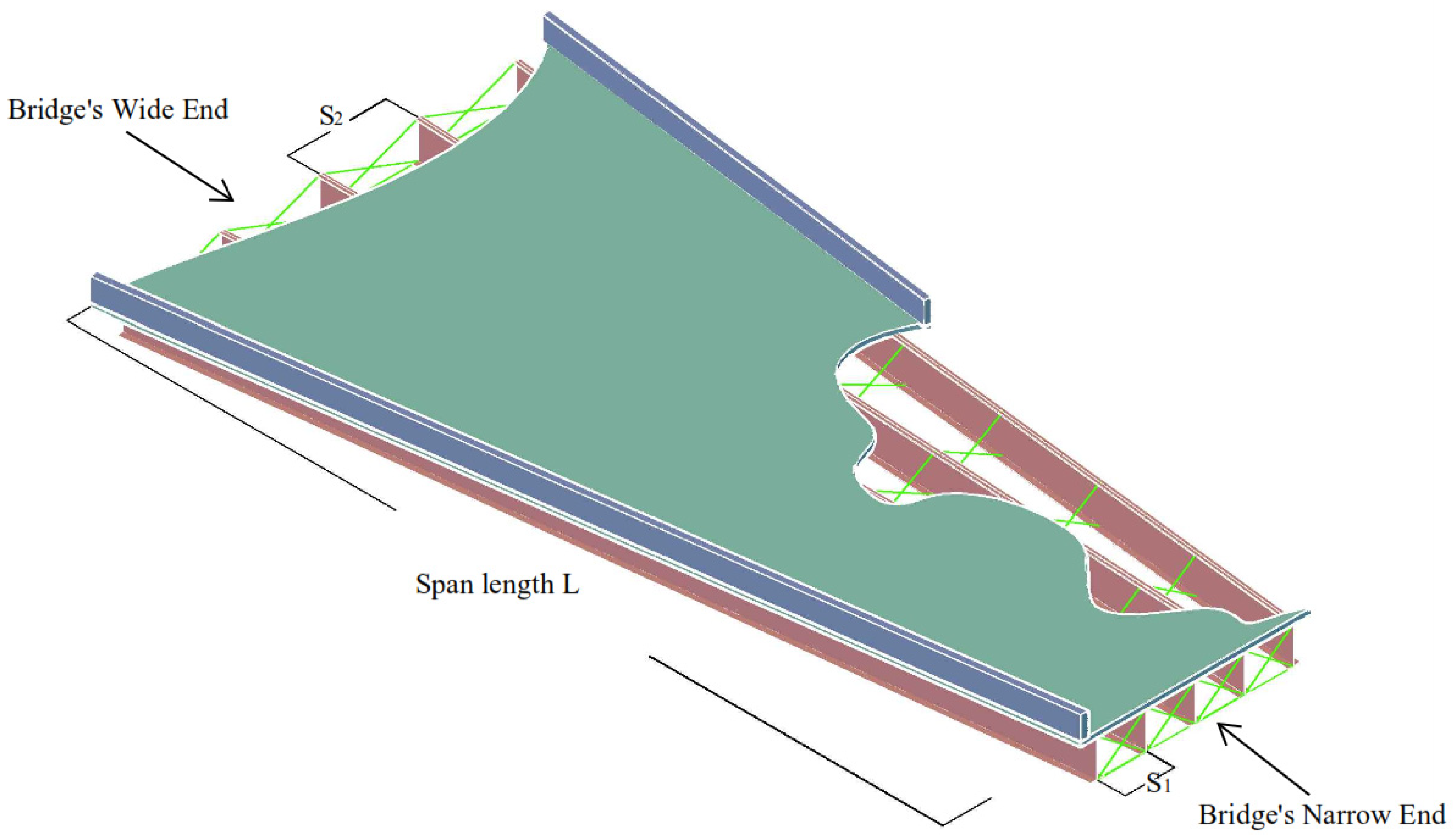
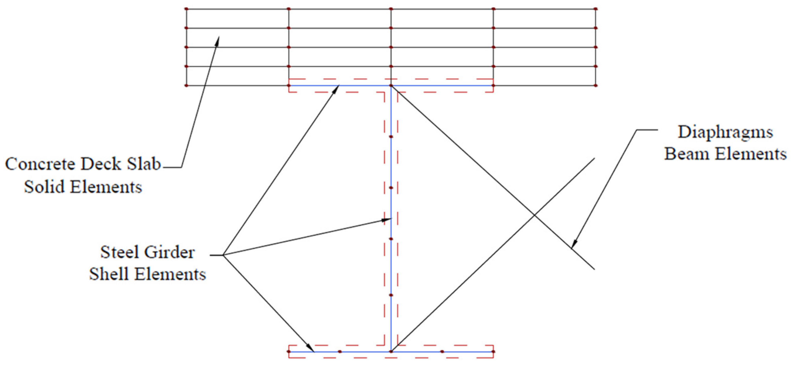
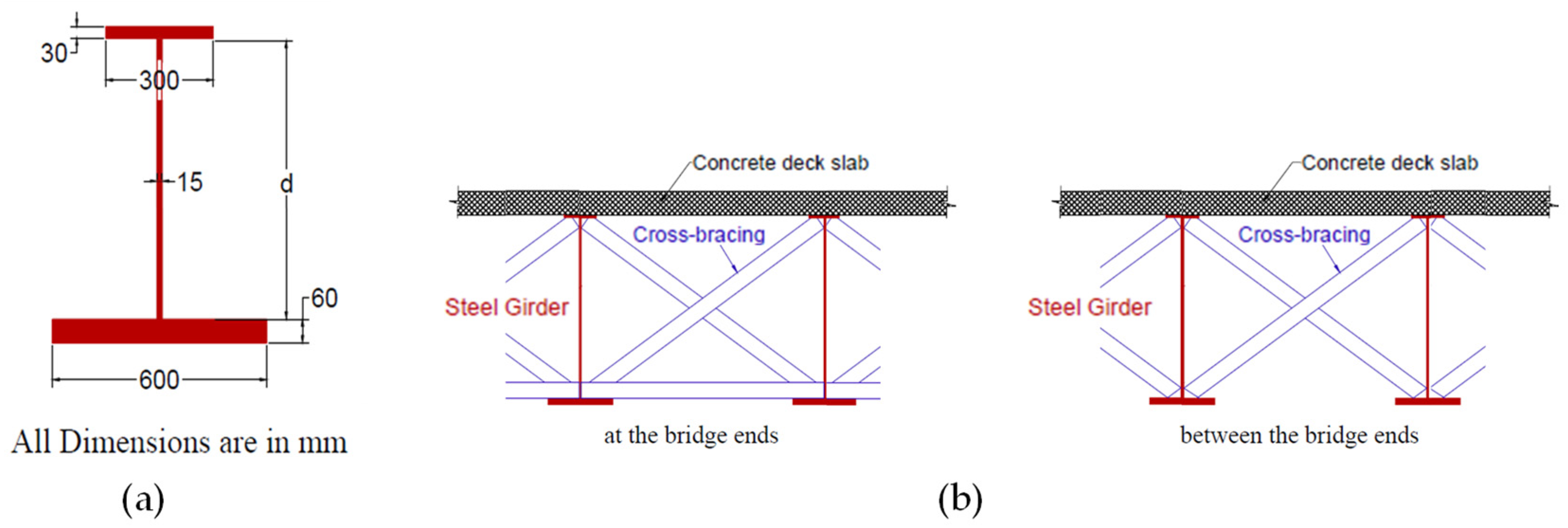
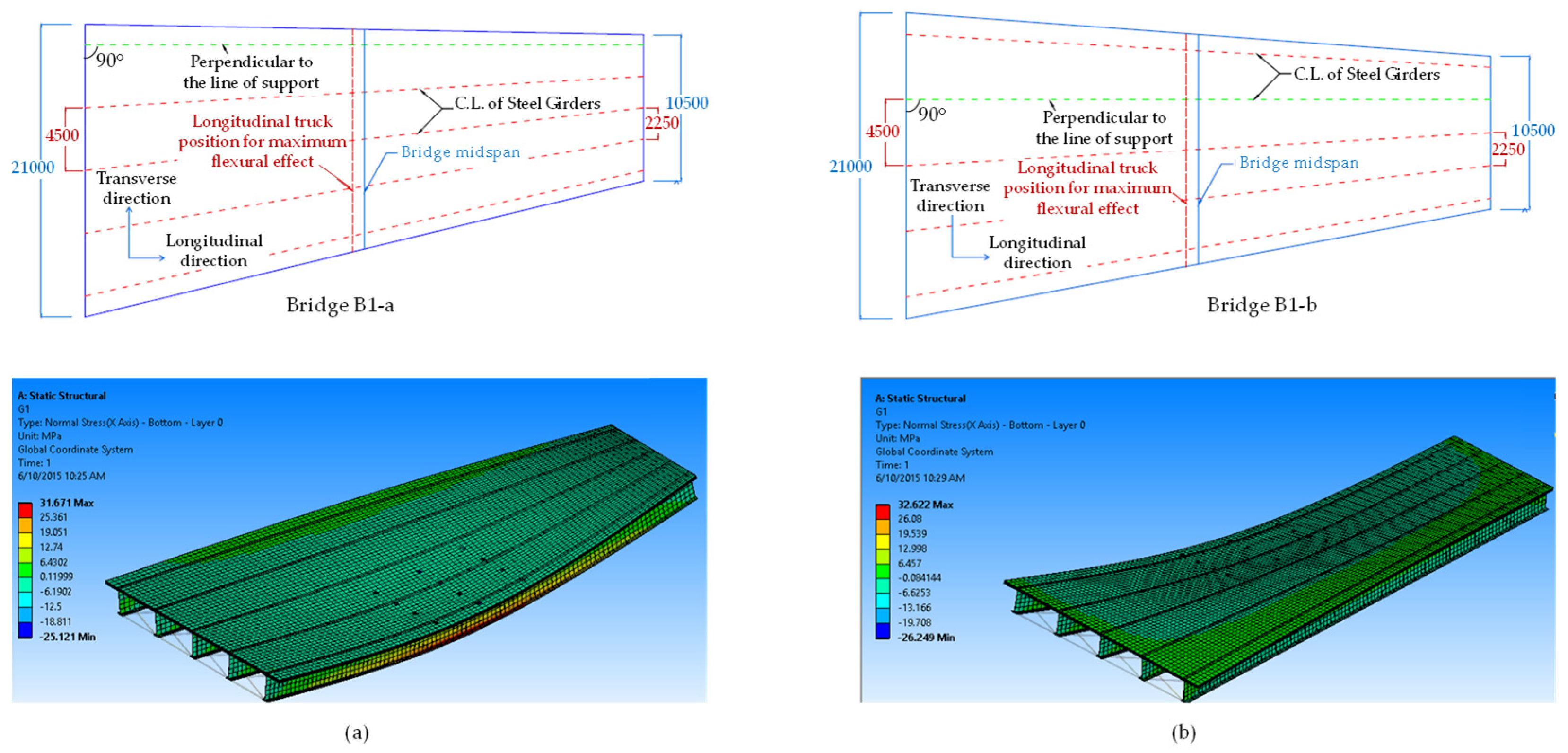
3.1. Finite Element Modeling

All the considered composite steel girder bridges in this investigation are modeled and analyzed within the elastic range by the ANSYS Version 14 software [15]. Over the past few decades, researchers working in the field of structural analysis of slab-on-girder bridges have used various approaches in their modeling that employ different types of finite elements and connectivity [4,16,17,18,19,20,21,22,23,24,25,26]. In this study, the girders are modeled with four-node shell elements for both flanges and the web (SHELL181). The material for all girders is steel which has a 200 GPa modulus of elasticity and 0.3 Poisson ratio. The uncracked concrete deck slab is modeled using multiple layers of eight-node solid elements (SOLID185) to account for the strain variation within these elements through the thickness. The deck slab material is concrete with a 25 GPa modulus of elasticity, which corresponds to approximately 30 MPa compressive strength, and 0.2 Poisson ratio. Diaphragms in the form of cross-bracing are modeled using two-node beam elements (BEAM188). The diaphragm material is steel with the same modulus of elasticity and Poisson ratio as the girders.

All the girders in the considered bridges are simply supported; they are simulated by a pin at one end and a roller at the opposite end. This means that the longitudinal translation of each girder is restrained at the pin location and unrestrained at the roller location. Live load is represented by the truck component of the AASHTO HL-93 live load, which is a common practice since neglecting the lane load component leads to conservative live load distribution results. Note that the truck is composed of three axles with 1.8 m gauge width, of which the front axle weighs 35 kN while the middle and rear axles each weigh 145 kN, with the distance between the front and middle axles being 4.3 m and between the middle and rear axles ranging between 4.3 and 9 m. The finite element model in this paper was verified by Hraib [27] using the results of the laboratory test on a full-scale bridge conducted by Fang at the University of Texas [28] and the field testing of the Creek Relief bridge in Texas carried out by Schonwetter [29]. Figure 2 provides a summary of the type of finite elements used to model the composite steel bridge girder.

3.2. Information on Parametric Study

A simply supported, splayed girder bridge with selected dimensions and material properties is chosen as a reference bridge. The considered parameters are the girder spacings (small spacing S₁ and large spacing S₂), and span length (L), slab thickness (t_s), cross-bracing spacing (D), girders’ web depth (d), and number of girders (n). The small and large girder spacing at the two extreme ends of the bridge were within the range of 1500–3000 mm and 3750–5250 mm, respectively. The span length varied between 30,000 and 50,000 mm, while the concrete deck slab thickness varied between 150 and 300 mm. The spacing of the cross-bracing was as small as 5 m and as large as the bridge length, i.e., no intermediate cross-bracing was present. The number of girders within the superstructure was 3, 5 and 7. While the dimensions of top and bottom flanges of the steel girders were kept constant, the depth of the web varied between 1400 and 2000 mm. The deck slab overhang ranged between 500–1250 mm at the supported narrow width of the bridge and 1000–1750 mm at supported wide width of the bridge. The range of variables considered in the study represent practical values that are encountered in real-life applications.

In the parametric study, one parameter is increased and decreased beyond the reference value, while all other parameters are kept unchanged. As the girders in this study are splayed by changing the spacing at the beginning and end of the bridge, a girder spacing parameter is changed four times using two different aspect ratios. The first aspect ratio is (S₂ − S₁)/L, which represents the degree of splayedness of the bridge, and by varying this parameter twice—once up and once down—the girder spacing is changed at one end and kept constant at the other. The second aspect ratio is the S₁/S₂ ratio, where the degree of splayedness ((S₂ − S₁)/L) is kept constant by changing the girder spacing of the end that was kept constant through the first aspect, which also generates two different bridges. The overhang cantilever width from the edge of the parapet to the centerline of the exterior girder (OH) is taken one-third of the interior girder spacing in all bridges, which is in line with common practice. The symbol OH₁ represents the overhang width at the narrower girder spacing end and OH₂ represents the overhang at the wider girder spacing end. A total of fifteen bridges are modeled by the computer program ANSYS to carry out the parametric study. The steel girders used in all the bridges considered consist of a 30 mm × 300 mm top flange, a 60 mm × 600 mm bottom flange, and a 15 mm thick web with varying girder depth (d), as shown in Figure 3a. The chosen cross-bracing consists of two or three equal-angle sections of 150 mm × 15 mm, as shown in Figure 3b. The concrete parapet cross-section is 300 mm wide and 1000 mm in height.

The fifteen bridges considered, shown in

Table 1. Characteristics of bridges considered in parametric study.

Bridge No.	S1 (mm)	S2 (mm)	L (mm)	ts (mm)	D (m)	n	d (mm)	OH1 (mm)	OH2 (mm)
B1	2250	4500	40,000	220	40	5	1700	750	1500
B2	3000	4500	40,000	220	40	5	1700	1000	1500
B3	1500	4500	40,000	220	40	5	1700	500	1500
B4	1500	3750	40,000	220	40	5	1700	500	1250
B5	3000	5250	40,000	220	40	5	1700	1000	1750
B6	2250	4500	40,000	150	40	5	1700	750	1500
B7	2250	4500	40,000	300	40	5	1700	750	1500
B8	2250	4500	40,000	220	5	5	1700	750	1500
B9	2250	4500	40,000	220	10	5	1700	750	1500
B10	2250	4500	40,000	220	40	3	1700	750	1500
B11	2250	4500	40,000	220	40	7	1700	750	1500
B12	2250	4500	40,000	220	40	5	1400	750	1500
B13	2250	4500	40,000	220	40	5	2000	750	1500
B14	2250	4500	30,000	220	30	5	1700	750	1500
B15	2250	4500	50,000	220	50	5	1700	750	1500

, are modeled using the finite element software ANSYS to determine the flexural and shear girder distribution factors for the critical interior and exterior girders. In all 15 cases, the line of support at the abutments is taken perpendicular to the central girder, which is the shortest in length among all the girders within the superstructure. In addition, two more bridges that are similar to the reference bridge B1 are considered, with the exception that the line of support at the abutments is either perpendicular to one of the exterior girders (B1-a) or one of the first interior girders (B1-b). The truck position is changed in each model to maximize the live load effect in the transverse and longitudinal directions for bending moment and shear force. The truck rotational angle within the bridge plan is also examined to maximize this effect, as elaborated in detail later in the paper.

3.3. Location of Maximum Dead Load Effect

Determination of the dead load effect in a flared girder within a bridge is a straightforward task. It starts by isolating an individual girder bounded by the tributary width of the slab supported by the girder. The major component of dead load includes the self-weight of the girder and part of the deck slab above it. As per the specifications, the weight of the parapets and wearing surface can be assumed to be shared equally by all the girders if they are placed after the concrete in the deck slab has cured and hardened. In addition to the distributed load along the length, the individual girder is also subjected to concentrated loads from the weight of the cross-bracings at their locations. If the latter load is taken as a small percentage of the girder’s self-weight, as is normally done in practice, the resulting dead load on the girder becomes uniformly distributed in the shape of a trapezoid along the girder’s length. The shear force and bending moment in the girder can then be computed by determining the support reactions, isolating a free body diagram of part of the girder at some distance away from one of the supports, and using statics if the structure is statically determinate. For a simply supported bridge, the maximum shear in the girder is equal to the support reaction at the bridge’s end, where the girder spacing is largest. The critical bending moment does not occur at the midspan due to the varying width of the bridge deck slab, which causes the critical flexural effect in the girder to be shifted toward the region with larger girder spacing, where the shear is zero. Figure 4 shows a single interior girder isolated from a simply supported splayed girder bridge and loaded by its self-weight, exclusive of the superimposed dead load, together with the corresponding shear and bending moment diagrams. The shift in the location of the maximum moment from midspan represents the location of zero shear. Conducting a three-dimensional finite element analysis on various splayed girder bridge systems yielded virtually the same result as the line element approach. Note that for the reference bridge B1, the self-weight of the steel girder is 5.43 kN/m, while the weight of the concrete deck slab over the tributary width is 11.65 kN/m at the smallest girder spacing and 23.3 kN/m at the largest girder spacing. For the interior girder in the reference bridge B1, this loading causes a maximum shear of 480.3 kN at the left support and a maximum bending moment of 4438.8 kN/m at 19,165 mm from the left support.

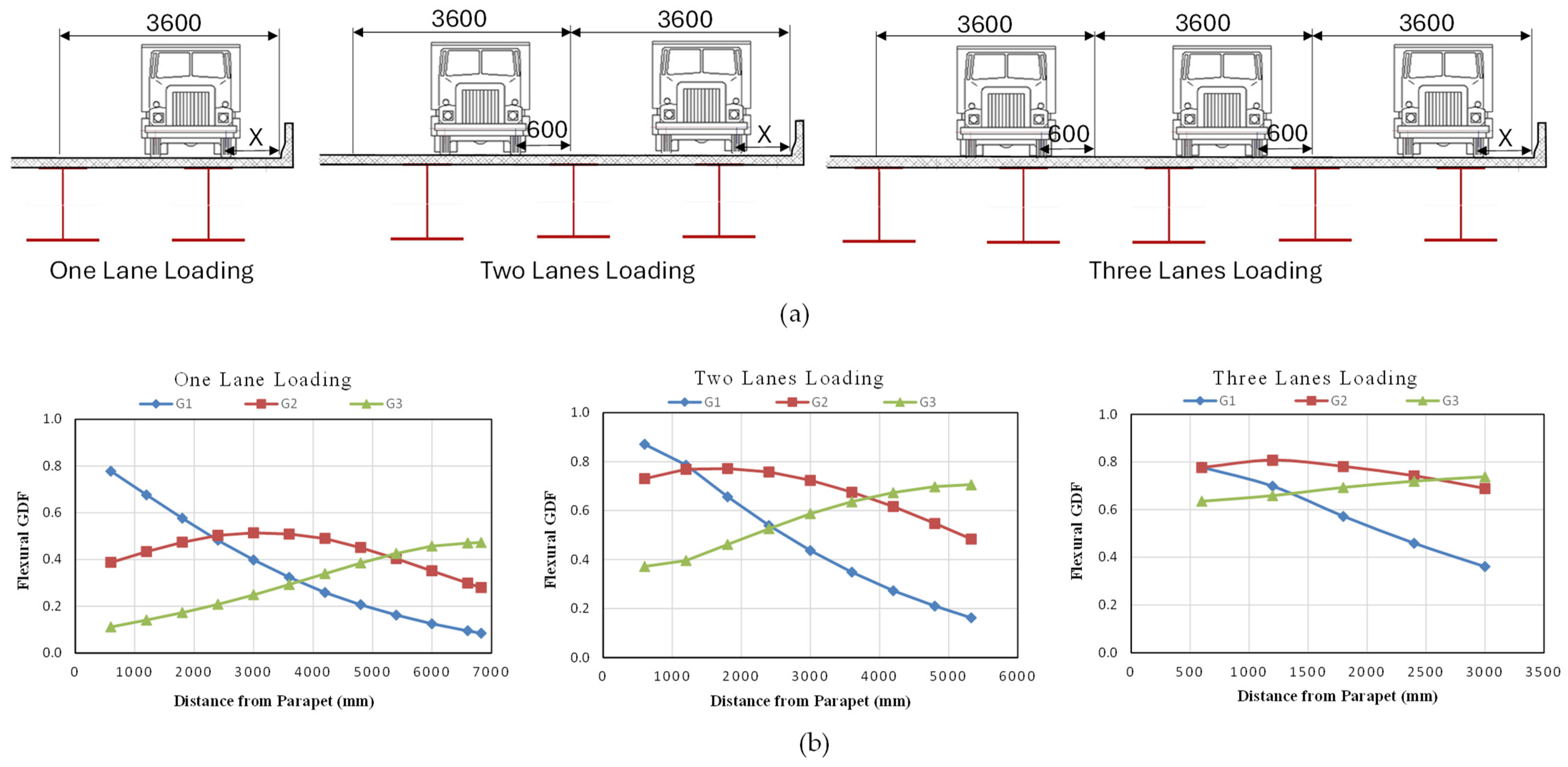
3.4. Truck Positioning and GDF

In this study, the girder distribution factor is calculated for flexure and shear in the exterior and interior girders due to the truck component of AASHTO HL-93 live load. The truck(s)’ position in the longitudinal and transverse direction is very critical to maximize the effect of live load in the bridge primary elements. Single truck positioning in the longitudinal and transverse directions, which maximizes the GDF for flexure and shear in the girders, is explained. Multiple truck positioning in the transverse direction follows a similar pattern, provided that each of the side-by-side trucks stays a minimum of 600 mm from the edge of the 3600 mm lane, as per the AASHTO requirements.

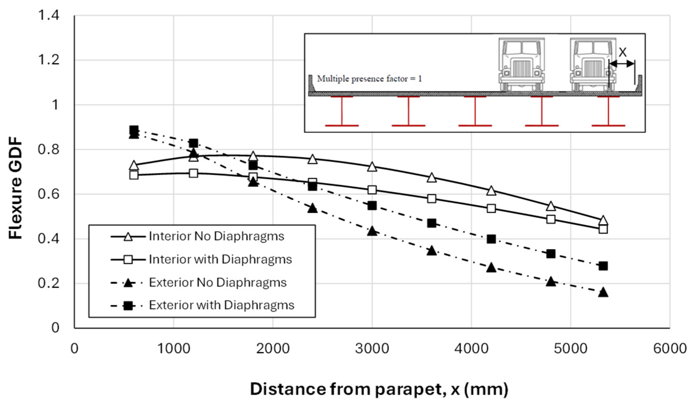
3.4.1. Longitudinal Truck Position

Based on the AASHTO LRFD specifications [1], no more than one truck is allowed to be placed within each lane on the bridge, but multiple side-by-side trucks in the transverse direction are permitted provided that appropriate multiple presence factors are considered. Since maximum shear force in the girders occurs at the support of the bridge with the larger girder spacing, critical truck positioning in this case requires placing the rear axle just off the support with the intermediate and front axles positioned at 4300 mm and 8600 mm away from the support, respectively. To maximize the bending moment in a simply supported bridge with parallel girders, the truck is generally placed at the midspan of the bridge, and by using an HL-93 truck, the middle axle is positioned at the midspan of the bridge. This moment is not necessarily the largest moment, but since the dead load moment occurs at the midspan of a regular bridge with a constant width, it is common practice to consider the combined load effect at the midspan. However, this is not the case in a splayed girder bridge, because the varying width of the bridge causes the maximum bending moment in the girders to be shifted away from the midspan toward the region with the larger girder spacing. In lieu of using an influence surface approach to determine the critical longitudinal truck location for maximum flexural effect in a splayed girder bridge, one truck is positioned symmetrically within the width of the bridge and the tensile stress at the bottom of the central girder is determined as a function of the longitudinal truck position. For reference bridge B1, the location of maximum flexure in the girder, determined by 3D finite element analysis of the entire bridge system under the critical longitudinal truck position, was found to be at 18,925 mm from the abutment that supports the wide part of the bridge, as shown in Figure 5. The obtained value is less than 1.3% of the 19,165 mm value, which represents the location of maximum flexural dead load effect. Based on the above finding, it seems practical to assume that the critical middle axle location of the truck(s) along the longitudinal axis for maximum flexure in a splayed bridge coincides with the location of maximum dead load flexural effect. Such an assumption is reasonable since the critical load effect in the girder is a combination of the influence of both dead and live loads. Furthermore, the longitudinal location of the truck(s) on the bridge is generally insensitive to the magnitude of the dimensionless girder distribution factor as long as the longitudinal truck location does not vary by much from the correct location.

3.4.2. Transverse Truck Position

The bridge is loaded by single or multiple side-by-side trucks placed within the transverse lanes to maximize the live load flexural and shear effects in the exterior or critical interior girder. The AASHTO LRFD specifications [1] account for the lower probability of simultaneous presence of multiple trucks over a bridge by employing a multiple presence factor. To find the maximum live load effect in the exterior or interior girders, different locations should be checked in the transverse direction for maximum effect in the member under consideration. The truck is first placed at a minimum clear distance from the edge of the interior face of the parapet and is then moved transversely in small increments toward the parapet on the opposite side of the bridge until the considered girder reaches the greatest live load effect.

In this study, variable spacing of the girders has an effect on truck positioning in the transverse direction, where both the position of the truck and the truck plan orientation angle affect the structural analysis results. By giving the truck the correct angle in the proper position, the live load effect can be maximized. Finite element analysis of the bridge systems showed that the truck orientation on the bridge influences both the interior and exterior girders but has a higher effect on the exterior girder, especially when the overhang width is large. By loading a splayed girder bridge with a truck oriented perpendicular to the line of supports, with a minimum wheel distance of 600 mm from the parapet, as required by AASHTO, only the wheel at the front or rear axle of the truck will maintain this minimum distance, while the other two axles will have a greater distance from the parapet, thus resulting in a lower flexural effect on the exterior girder. If the truck is oriented parallel to the parapet with a constant wheel distance of 600 mm from the parapet, the flexural effect of the truck on the exterior girder will be maximized because all of the truck wheels will contribute more toward the load effect in the girder. With regard to an interior girder, maximum flexural load effect is attained if the truck axle is oriented perpendicular to the centerline of the girder under consideration, as shown in Figure 6.

To maximize the shear effect due to live load, the truck is placed just off the support at the end of the bridge in the longitudinal direction. However, like in flexure, the truck should be moved in the transverse direction starting from 600 mm away from the face of the parapet until the maximum effect is reached in the girder under consideration. Finite element analysis showed that rotating the truck to maximize the shear effect was not critical in the interior girders, where keeping the truck perpendicular to the end support produced the maximum shear effect for such girders. Alternatively, orienting the truck in a position parallel to the parapet resulted in the maximum shear effect in the exterior girder.

3.4.3. Girder Distribution Factor

At each step of transverse truck positioning for the case of flexure at midspan, longitudinal normal stresses at the bottom flange of all girders due to flexure are recorded along a straight line through the girders, representing the truck’s chosen longitudinal position. The GDF for flexure is then calculated for each girder as a ratio of its stress at the extreme fibers to the summation of stresses in all girders at the critical location, since in elastic analysis, the normal stress due to flexure is proportional to bending moment. The GDF for shear is computed using the ratio of the support reaction of the girder under consideration to the summation of the reactions of all girders at the loaded end of the bridge. Equations (8) and (9), presented below, are used in this study to calculate the GDF for flexure and shear, respectively, in both interior and exterior girders, using the finite element results with consideration of the AASHTO multiple truck presence factor [1].

Flexure in interior or exterior girders:

$${GDF}_j={\displaystyle \frac{Nm{\sigma }_j}{\sum _{i=1}^n{\sigma }_i}}$$

(8)

Shear in interior or exterior girders:

$${GDF}_j={\displaystyle \frac{Nm{R}_j}{\sum _{i=1}^n{R}_i}}$$

(9)

where N = number of loaded lanes, m = multiple presence factor, σ_j = normal stress due to flexure at the bottom flange of girder j (MPa), σ_i = normal stress due to flexure at the bottom flange of girder i (MPa), R_j = support reaction at girder j (N), R_i = support reaction at girder i (N), and n = number of girders. For the case of flexure, all stresses obtained from the 3D finite element analysis at the bottom flange of the girders, where there are five nodes, are weighted average stresses. For the case of shear, the vertical reactions are taken exactly at the supported nodes underneath the individual girders.

4. Detailed Analysis of Reference Bridge B1

In this section, the method outlined earlier for determining the girder distribution factor is illustrated in detail for the reference splayed girder bridge B1. The 40 m simply supported bridge is composed of five girders that are spaced at 4.5 m at the wide end and 2.25 m at the narrow end, with the overhang width being one-third of the girder spacing. The bridge has a 220 mm thick concrete slab and contains diaphragms in the shape of cross-bracing only at the supports. The structural layout, cross-section dimensions, and finite element model are shown in Figure 7.

Each splayed highway bridge modeled in this study was loaded for maximum flexure and shear effect by moving one, two, and three trucks within their lanes in the transverse direction to maximize the live load effect in the girders. Moving the side-by-side trucks incrementally from one parapet to the opposite side leads to changes in the flexural and shear GDF values among the bridge girders. Figure 8 shows the load effect in the reference bridge due to two side-by-side trucks longitudinally positioned near the midspan, considering the longitudinal normal stresses in the bottom flanges and vertical shear stresses in the webs of the girders.

For the reference bridge under consideration, Figure 9 shows the flexural GDF values plotted against the distance of the truck from the parapet in cases of one, two, and three trucks with consideration of the appropriate multiple presence factors. The results indicate that critical flexure in the first interior girder G2 led to the highest GDF (equal to 0.808) when compared with the central interior girder G3. Furthermore, the exterior girder G1 had the highest GDF among all the girders—equal to 0.871. For flexure, the overall GDF value was governed by two-lane loading for the exterior girder, and by three-lane loading for the interior girders. Note that the girder designation (G1, G2, and G3) has been presented earlier in Figure 5b.

For the case of shear load effect in the girders, two cases of in-plan truck orientation were checked because maximization of the GDF for the interior girders required a different truck placement to that for the exterior girders. One of the two truck placements consisted of the trucks’ lines of wheels being parallel to the parapet (Case 1), while the second consisted of the trucks’ axles being perpendicular to girder under consideration (Case 2). The results, shown in Figure 10 as a function of the lateral distance from the parapet, show that the maximum shear GDF for the exterior girder is governed by one-lane loading, while for the interior girder, it is governed by two-lane loading. This finding is not in agreement with the flexural effect, where three-lane loading governs the GDF for the interior girders. Similar to the flexure case, shear GDF in first interior girder governs the central interior girder. Compared to the flexural GDF, the shear GDF is larger in magnitude, which is an expected result since there is little differential vertical deflection among the girders near the support, leading to little load sharing. The critical shear GDF is 1.036 for the exterior girder and 1.313 for the interior girder, resulting in a 26.7% difference between the two values.

All bridges considered in this study and shown in Table 1 are symmetrical in plan around the centerline of the bridge, which results in the central girder(s) being the shortest and the exterior girders being the longest in length. Therefore, to ensure that the results of this study are applicable to different in-plan splayedness orientations, two bridges similar to the reference bridge are modeled, but with a different splayedness orientation, as shown in Figure 11. For the first bridge (B1−a), the girder that is perpendicular to the line of supports is the exterior girder. In the second bridge (B1−b), the first interior girder is the one perpendicular to the line of supports. Finite element models are developed for each of the two alternative splayed girder bridges, B1−a and B1−b, and the same loading procedure followed in the reference bridge for maximizing flexural effect is applied for these two bridges, with consideration of the same longitudinal truck(s)’ position. Results from the 3D finite element analysis showed the most critical GDF values, whether in the exterior or in the first interior girders, negligibly changed (by less than 1%) in the two alternative bridges B1−a and B1−b compared to the reference bridge B1. Based on the above, it can be concluded that lack of symmetry of the girder splayedness is not an important factor in the analysis of splayed girder bridges.

After presenting the finite element results for the reference bridge, an approximate procedure is proposed and demonstrated for computing the GDF for both flexure and shear in interior and exterior girders. This method avoids the need for a refined method of analysis as it utilizes a one-dimensional beam analysis. The procedure is based on the AASHTO LRFD formulas used to calculate the GDF for flexure and shear in slab-on-parallel-girder bridges. The objective of this procedure is to find out if such a simple method can be reasonably used to determine the load effect in the girders of such irregular bridges without the use of three-dimensional finite element analysis.

The general concept of the approximate approach is to compute the GDF for interior or exterior girders considering the actual girder spacing at each truck axle position along the bridge using the AASHTO LRFD formulas [1]. Each of the three GDF values at the front, middle, and rear axles is then multiplied by the corresponding axle load, and structural analysis of a single composite girder is carried out to determine the live load flexural effect on the interior girders from Equations (1) and (2) or the shear effect on the interior girders from Equations (4) and (5) at the critical location. For the live load effect on the exterior girders, Equations (7) and (8) can be used to determine the GDF for cases of flexure and shear, respectively. The same single composite girder is loaded again with the full AASHTO truck load, without multiplying it by the GDF, and structural analysis is used again to obtain the critical flexural or shear effect in the girder at the critical location. Finally, the equivalent GDF is obtained as the ratio of the maximum live load effect due to multiplying the load by the GDF corresponding to the live load effect under the full truck load without any factors. The outlined approach consolidates the three hand-calculated GDF values at the three different axle locations into one quantity at the critical location for flexure or shear. Such an approach makes it convenient to compare the AASHTO results with the finite element findings obtained with the help of Equations (8) or (9).

To test the proposed approximate method, the equivalent GDF values for the reference bridge B1 are calculated and compared with the finite element outcome. Figure 12a shows the flexural results of the equivalent GDF by the AASHTO formulas (referred to as “Equ AASHTO”) with the finite element outcome (referred to as “FEM”). On the other hand, Figure 12b presents the shear results of the equivalent GDF by the AASHTO formulas and the finite element result, together with the equivalent GDF by the lever rule (Referred to as “Equ LR”). To apply the lever rule, a section of the superstructure composed of the slab supported on the girders is taken, a hinge is assumed to develop in the slab over each interior girder, side-by-side axles of trucks are applied with their appropriate multiple presence factors, and the statically determinate problem is solved for the reaction of the considered girder as a fraction of the axle load using statics.

For flexure in the reference bridge, the results show that the equivalent GDF values for the critical interior and exterior girders are about 4% and 3% higher than the corresponding finite element results. For shear, the finite element results are 5% and 18% higher than the equivalent GDF by AASHTO formulas for the interior and exterior girders, respectively. Use of the lever rule for determining the shear GDF led to higher values than those obtained with the AASHTO formulas, thus leading to values that were closer to the finite element results. For the shear GDF in interior girders, the lever rule matched the finite element outcome and yielded about 6% higher values for the exterior girders.

Based on the above, the suggested approach of determining the live load effect in interior and exterior girders subjected to flexure or shear seems reasonable and safe. However, before fully accepting the approximate approach, validation of the suggested procedure should be extended to bridges with different geometries, which is discussed in the next section.

5. Parametric Study

To verify the general applicability of the outlined equivalent GDF approach for flexure and shear in interior and exterior girders, a parametric study is followed. This study considers different aspects that strongly affect the behavior of splayed girder bridges. These parameters are represented in the 15 bridges (B1–B15) listed in Table 1, which include variations in girder spacing S, slab thickness t_s, cross-bracing spacing D, number of girders n, girder web depth d, and span length L.

Table 2. Range of variables considered in the parametric study.

Parameter	Girder Spacing Parameter				Slab Thickness ts (mm)	Cross-Bracing Spacing D (m)	No. of Girder n	Girder Depth d (mm)	Span Length L (mm)
	(S2 − S1)/L *		S1/S2
	S1 (mm)	S2 (mm)	S1 (mm)	S2 (mm)
Reference (B1)	2250	4500	2250	4500	220	40	5	1700	40,000
Lower value	1500	4500	1500	3750	150	5	3	1400	30,000
Upper value	3000	4500	3000	5250	300	10	7	2000	50,000

* Bridge length = 40,000 mm.

shows the ranges of these parameters, each varied from the specified values of the reference bridge B1. For each parameter, two additional configurations are created—one with a lower value and one with a higher value—while keeping the rest constant. This results in a total of 15 splayed girder bridges with different parameters to be considered in this study. It can be said that each parameter is studied using three bridges, including the reference bridge.

Since the girder spacing is the most critical parameter that greatly impacts the live load distribution, two splayedness measures are considered in the parametric study. The first one is the splayedness ratio (S₂ − S₁)/L, which represents the degree of splayedness of the bridge, and the second one is the girder spacing ratio S₁/S₂, which considers the girder spacing without the span length. In the latter case, the splayedness ratio (S₂ − S₁)/L is kept constant while varying the S₁/S₂ ratio. Hence, four bridges in total are considered for the effect of girder spacing—two for each aspect.

5.1. Flexure in Girders Due to Live Load

In this section, the flexural effect in the splayed girders is considered and discussed with consideration of various parameters, such as the girder spacing, deck slab thickness, spacing of cross-bracing, and other parameters.

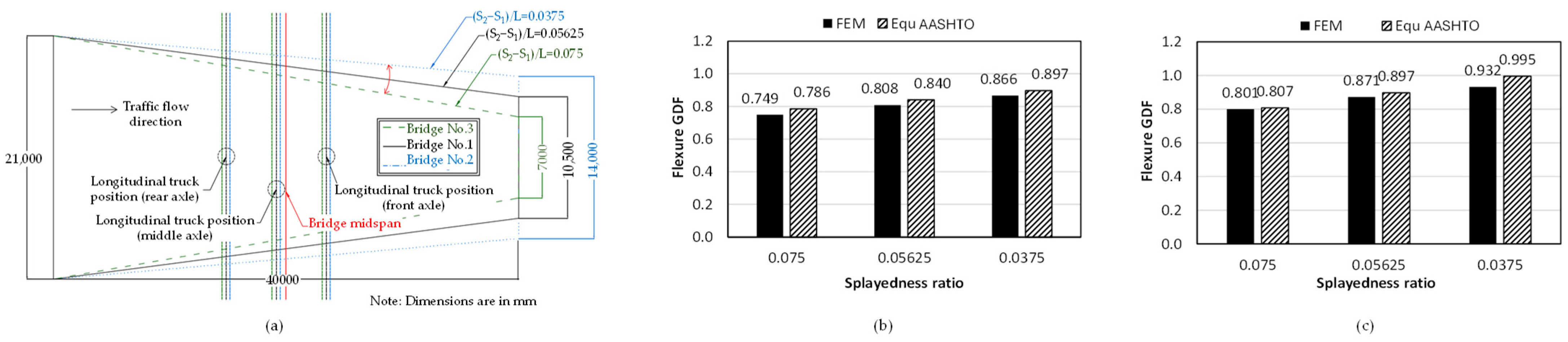
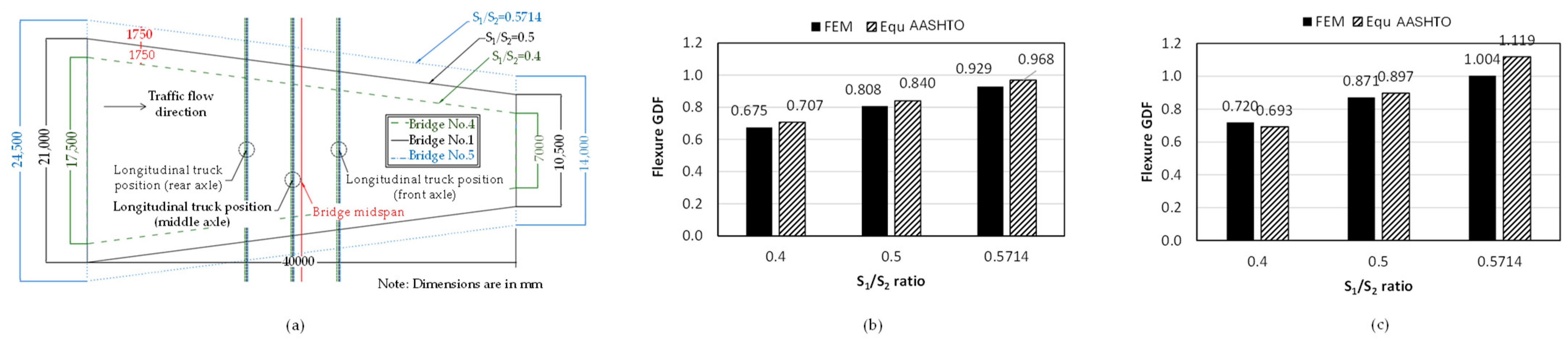
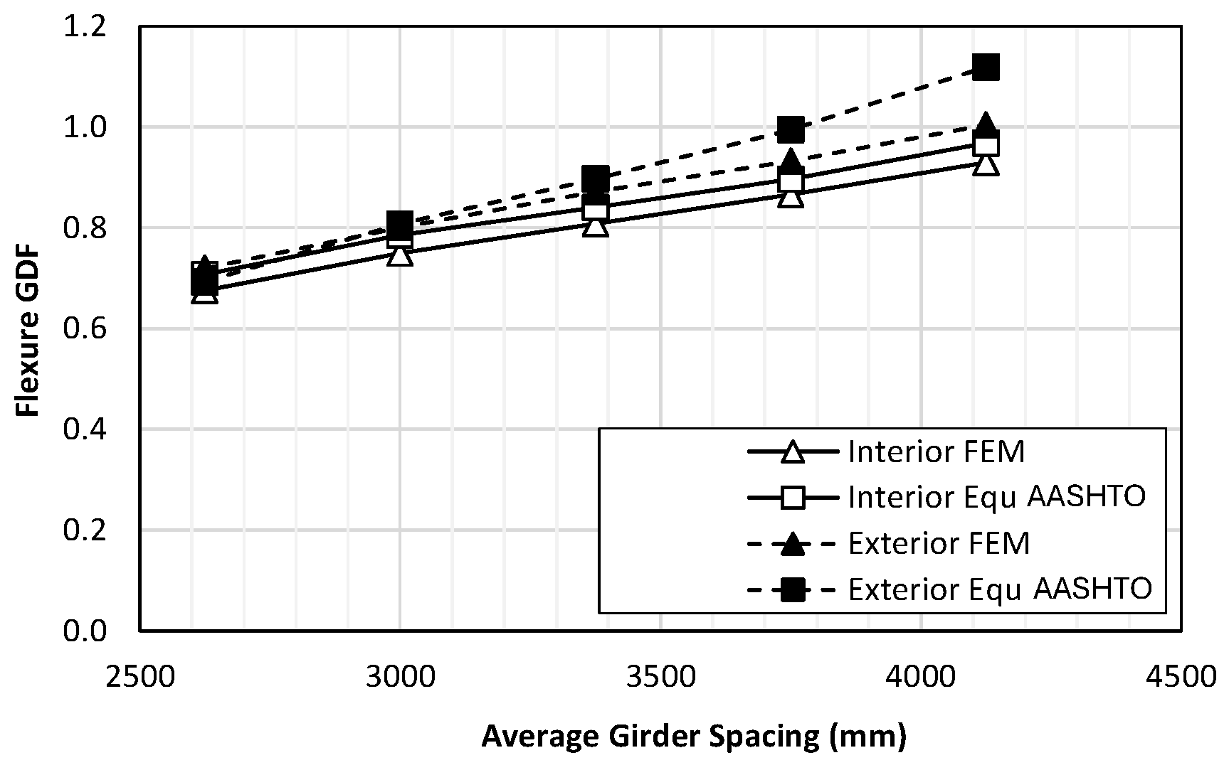
5.1.1. Effect of Girder Spacing

As mentioned before, the influence of the girder spacing on the structural behavior was examined using two distinct approaches—first, by examining the splayedness ratio (S₂ − S₁)/L effect, and second, by exploring the girder spacing ratio S₁/S₂ effect—in order to gain a better insight into the effect of the change in the girder spacing along the bridge span.

Bridges B2 and B3 in Table 1 were developed based on the reference bridge B1 to observe the effect of the splayedness ratio (S₂ − S₁)/L on the structural behavior. Figure 13a provides a plan view showing bridge B1 in black, B2 in blue, and B3 in green. Starting with the reference bridge B1, the girder spacing at the wide end was kept constant, while the spacing at the narrow end was adjusted to vary the splayedness ratio—increasing it by 33% to form bridge B2 and decreasing it by 33% form bridge B3. It should be noted that increasing the splayedness ratio leads to a reduction in girder spacing along the span, while decreasing the ratio leads to increased girder spacing. The finite element results in Figure 13b show that increasing the splayedness ratio by 33% leads to a 7.254% reduction in the flexure GDF for interior girders, while decreasing it by 33% leads to an almost equal increase in the GDF. For exterior girders, increasing the splayedness ratio by 33% results in an 8.12% reduction in the flexure GDF value, while decreasing it by 33% causes the flexure GDF to increase by 6.93%, as shown in Figure 13c. The bridges were also analyzed using the AASHTO-based equivalent GDF approach outlined earlier, allowing us to find the flexure GDF values with a simple approach and compare them to the finite element outcome. Figure 13b,c show that for the interior and exterior girders, the equivalent AASHTO flexure GDF values for the three bridges are very close to the finite element values, with reasonable conservatism, amounting to a maximum percentage difference of less than 5% for all the considered bridges.

Bridges B4 and B5 were developed by modifying reference bridge B1 with the aim of assessing the effect of the girder spacing ratio S₁/S₂ on the structural response. To effectively examine this ratio without interference from the splayedness ratio, the (S₂ − S₁)/L ratio for all three bridges was set to be constant—equal to 0.05625. Figure 14a shows a plan view for bridges B1, B4, and B5. By decreasing the girder spacing of the reference bridge at any section along the span by 750 mm and increasing it by 750 mm, the S₁/S₂ ratios for bridges B1, B4, and B5 become 0.5, 0.4, and 0.571, respectively. The finite element results for the interior girders, shown in Figure 14b,c, indicate that increasing the S₁/S₂ ratio by 14.3% leads to a 15.05% increase in the GDF, while decreasing the S₁/S₂ ratio by 20% leads to a 16.39% reduction in the GDF. For the exterior girders, increasing the S₁/S₂ ratio by 14.3% leads to a 15.17% growth in the GDF, while decreasing the S1/S₂ ratio by 20% leads to a 17.41% reduction in the GDF. Note that although the S₁/S₂ ratio increased by 14.3% and then decreased by 20%, these changes resulted in almost equal absolute percentage changes in the GDF for interior and exterior girders, as they caused the same changes—increasing or decreasing—in girder spacing value at any particular section along the bridge length. However, the small difference between the percentage growth and reduction in the GDF—whether in the interior or exterior girder—is due to minor changes in the truck(s)’ longitudinal location between bridges B1, B4, and B5 in order to maximize the GDF for flexure. Figure 14b,c also include the equivalent AASHTO GDF for the interior and exterior girders for all three bridges. It is clear that the GDF values obtained by finite element analysis and the AASHTO formulas are very close in the interior and exterior girders, with an adequate level of conservatism. The only case in which there is a somewhat large deviation (about 11%) between the two analysis methods is observed for exterior girders in the bridge in which the S₁/S₂ = 0.5714; nevertheless, this deviation is on the safe side.

Before the discussion about the influence of girder spacing on the live load distribution characteristics of splayed girder bridges under flexure is completed, we consider one more parameter on the subject. Figure 15 shows the change in the flexural GDF as a function of the average girder spacing, determined by S_avg = (S₁ + S₂)/2, for bridges B1, B2, B3, B4, and B5. As expected, the average increase in the girder spacing always leads to higher GDF values. For the bridges considered, in which the overhang width is equal to one-third of the girder spacing, the exterior girder GDF was consistently larger than the corresponding interior girder GDF. The equivalent AASHTO GDF expressions closely match the finite element results, particularly for bridges with short and medium average girder spacings. Note that other splayed girder bridges with a smaller deck slab overhang length than the considered value in the study may lead to a more critical load effect in the interior girders than in the exterior ones.

5.1.2. Effect of Deck Slab Thickness

The influence of slab thickness on girder splayedness is examined in this study by using a 33.3% lower and 33.3% higher value of the concrete deck slab thickness compared with reference bridge B1. Bridges B6 and B7 are identical to bridge B1, except for their slab thickness being 150 mm and 300 mm, respectively. The finite element models for the considered bridges showed that for the interior girders, increasing the 225 mm slab thickness by 33.3% leads to a 5.2% decrease in the flexure GDF value, while decreasing it by the same percentage results in a 6.7% increase in the GDF value. This is because increasing the slab thickness results in a stiffer member, which transfers the truck(s)’ load more uniformly across the supporting interior girders and leads to less differential deflection between the girders. This results in more load sharing among the girders, decreasing GDF in bridge B7. In contrast, the thinner slab in bridge B6 results in less load sharing, which leads to a higher GDF. However, the exterior girders did not act in a similar way to the interior girders, where increasing or decreasing the slab thickness by 33.3% compared to the reference bridge resulted a change in GDF of only about 1%. The reason the GDF of the exterior girders was not significantly affected by the slab thickness can be explained by the fact that the load on these elements is mainly due to a single truck placed near the overhang or in the vicinity of the girder region. This mechanism is equivalent to a statically determinate element (in this case, a cantilevered overhang) where slab thickness does not contribute to the load effect. Figure 16 shows the finite element and equivalent AASHTO GDF values versus the slab thickness for critical interior and exterior girders in the considered bridges. The equivalent AASHTO GDF approach showed the same trend for the interior girders as the finite element results but exhibited a different tendency for the exterior girders. This is because the GDF is based on the AASHTO LRFD formulas, where the exterior GDF is a product of the interior girder GDF and a factor related only to the overhang distance, resulting in a constant value for all the considered bridges. Comparing the outcome of the refined method with that of the hand calculations showed that the equivalent AASHTO GDF for both the interior and exterior girders yielded slightly conservative results compared to the finite element values in most cases. As the slab thickness increased, the difference between the finite element and equivalent AASHTO GDF factors diminished.

5.1.3. Effect of Cross-Bracing

The AASHTO formulas used to calculate the GDF were developed based on bridge models not containing diaphragms or cross-bracings [30]. Therefore, the reference bridge in this study is assumed to have cross-bracing only at the ends of the bridge (40 m). However, two other bridges with different cross-bracing spacings are developed to address the cross-bracing effect on the structural behavior of splayed girder bridges. Bridge B8 has a cross-bracing spacing equal to 5 m, while bridge B9 has a cross-bracing spacing equal to 10 m. Figure 17 shows the change in GDF due to the movement of two trucks in adjacent lanes in the transverse direction for two bridges—one in which the bracings are located at the supported ends only (reference bridge B1), and the other in which the bracings are located at 5 m intervals along the bridge (bridge B8). It is clear from the results that the fraction of flexural live load in the interior girder for the bridge without bracing is higher than in the corresponding bridge with bracing. In contrast, the presence of cross-bracing in bridge B8 resulted in higher GDF values in the exterior girders than those resulting from the same bridge without cross-bracing (bridge B1). Adding cross-bracing to a bridge results in more uniform deflection across all girders, thus increasing load distribution among the interior girders and leading to a lower GDF. However, increasing the rigidity of the cross-section with the addition of cross-bracing increases the effect of rigid body rotation on the exterior girder as a result of the eccentricity of the truck load in the transverse direction about the bridge centerline, which results in a higher GDF in the exterior girders.

Finite element analysis showed that the presence of intermediate cross-bracing affects the GDF values, although the spacing of the cross-bracing is not a significant parameter. Adding cross-bracing to the reference bridge slightly increased the GDF of the exterior girder by up to 2% while reducing GDF of the interior girder by about 8%. Moreover, the analysis showed that rigid body rotation of splayed girder bridges is less pronounced compared to that in parallel girder bridges. This is because transverse eccentric truck positioning has a reduced effect due to the resistance of flared girders to superstructure twisting. Note that the AASHTO equivalent GDF expressions do not account for the presence or spacing of cross-bracing. Therefore, all three bridges—B1, B8, and B9—with different cross-bracing spacings have the same equivalent AASHTO GDF, as shown in Figure 18. Comparing this value for interior or exterior girders with the finite element outcome showed that the equivalent AASHTO GDF is a good predictor of the flexural live load distribution. Note that the rigid body rotation method for finding the equivalent GDF for the exterior girders resulted in a high value equal to 1.023, far exceeding the findings of the finite element analysis and the AASHTO approximate approach. Hence, such an approach is not recommended for splayed girder bridges since it results in an unreasonably higher load effect than the refined method.

5.1.4. Effect of Other Parameters

In this section, the number of girders, girder depth, and the span length of a splayed girder are considered to check the validity of using the AASHTO flexural GDF at the respective axle locations to determine the bending moment in the girders.

By reducing the number of girders in reference bridge B1 from five to three and increasing them from five to seven, while keeping all parameters—including the girder spacing—constant, bridges B10 and B11 are generated, respectively. It is clear from the finite element results of Figure 19 that the number of girders in a splayed girder bridge affects the GDF of the exterior girders more than the interior girders (8.5% versus 2.5% maximum difference between the extreme values). Although the AASHTO GDF formulas do not consider the number of girders explicitly in a bridge, the specifications suggest using the lever rule if the number of girders is three, as is the case in bridge B10. However, for consistency, the equivalent GDF is used for all bridges in the study, which results in an equal equivalent GDF in all three bridges with different numbers of girders. The results show that the AASHTO GDF provides a good predictor of the flexural effect in the girders, especially when the number of girders is not excessively large. It should be noted that use of the lever rule to compute an equivalent GDF resulted in much higher values than the finite element outcome, where in the interior girders, the GDF value was equal to 1.14, and in exterior girders, it was equal to 1.045.

In this study, the stiffness of the girder was adjusted by changing the depth of the steel girder web in the considered reference bridge. Bridges B12 and B13 were created by reducing the web depth of the 1700 mm girder in the reference bridge by 300 mm and increasing it by the same amount, respectively. Note that the girder level of rigidity in AASHTO is accounted for by the stiffness factor K_g, presented in this paper as Equation (3). The finite element findings shown in Figure 20 confirm the increase in the GDF with increased girder depth, especially for the interior girders, though the increase in GDF is not very significant. The AASHTO equivalent GDF follows the same trend and provides a safe upper limit to the results of the refined analysis.

B14 and B15 were generated by decreasing and increasing the 40 m simple span length of reference bridge B1 by 25%, respectively. Note that changing the bridges’ span length affects the splayedness angle of the bridge and consequently the girder spacing at the truck axle critical locations for maximum flexural effect, albeit not by much. Figure 21 shows that an increase in the span length has a favorable influence on the interior girders’ GDF, but not on that of the exterior girders. The AASHTO GDF expressions at the location of the axles are also capable of matching the finite element trend for the interior girders, but not the exterior girders, since the AASHTO exterior girder GDF is a result of a factor that is a function of the overhang width multiplied by the GDF of the interior girder. Nevertheless, the difference between the finite element and AASHTO results is insignificant.

5.1.5. Summary of Flexural Results

In summary, the presented results showed that for all of the fifteen splayed girder bridges analyzed in flexure, the equivalent GDF based on the AASHTO formulas for flexure were, for the most part, slightly larger than the GDF values obtained by finite element analysis. Figure 22 compares both methods with regard to the flexural GDF of critical interior and exterior girders. While there are very few cases in which the equivalent AASHTO GDF slightly underestimates the GDF values obtained by finite element analysis, these cases are nevertheless very close to each other. Hence, it can be concluded that for all practical purposes, the use of the flexural GDF AASHTO formulas with girder spacings corresponding to the locations of the truck axles is a good approach for analyzing splayed girders in flexure. This approach, which depends on a one-dimensional beam analysis, is simple and straightforward and eliminates the need for refined analysis, which is often costly and time-consuming, and yields outputs that are difficult to interpret.

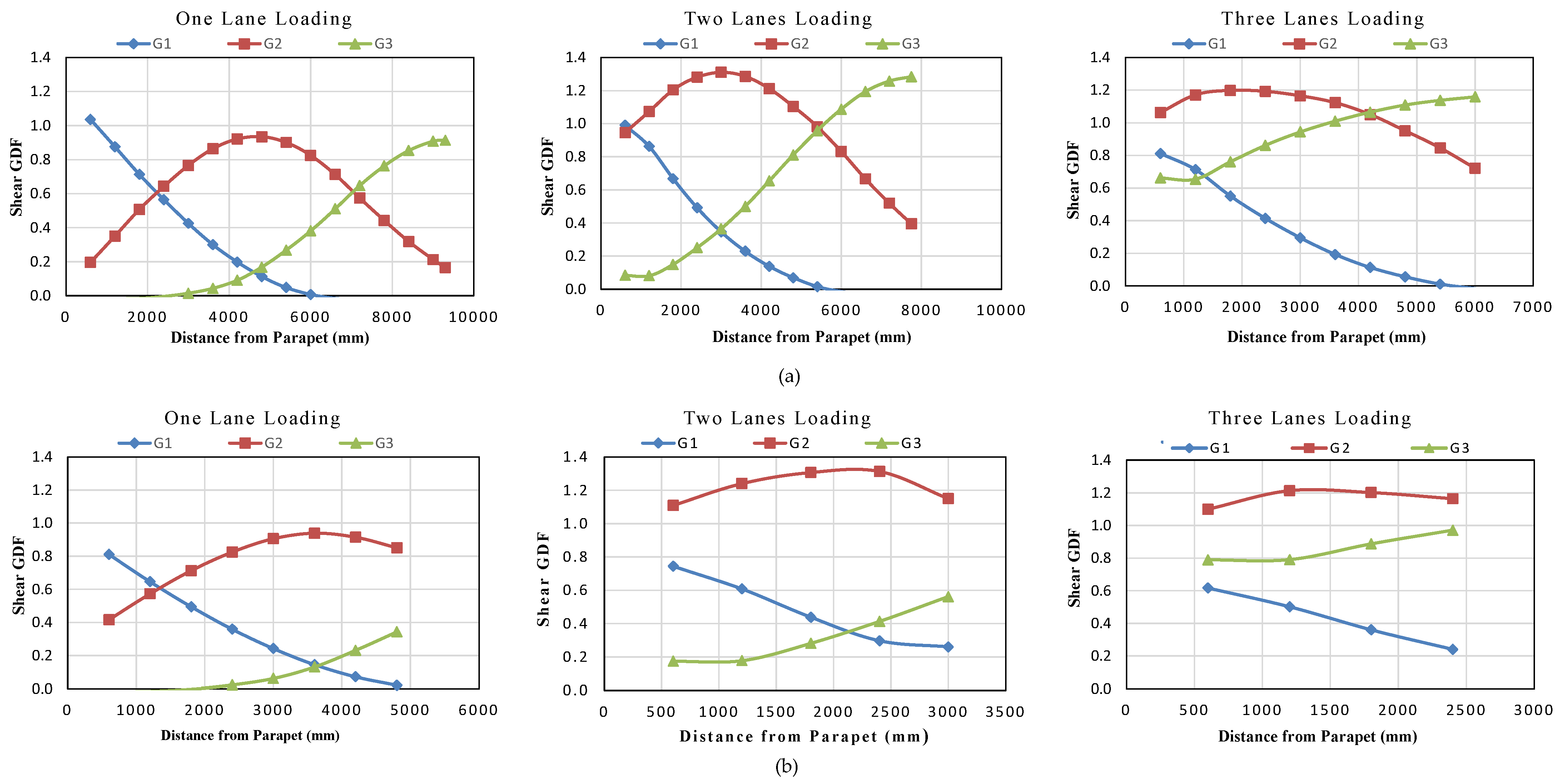
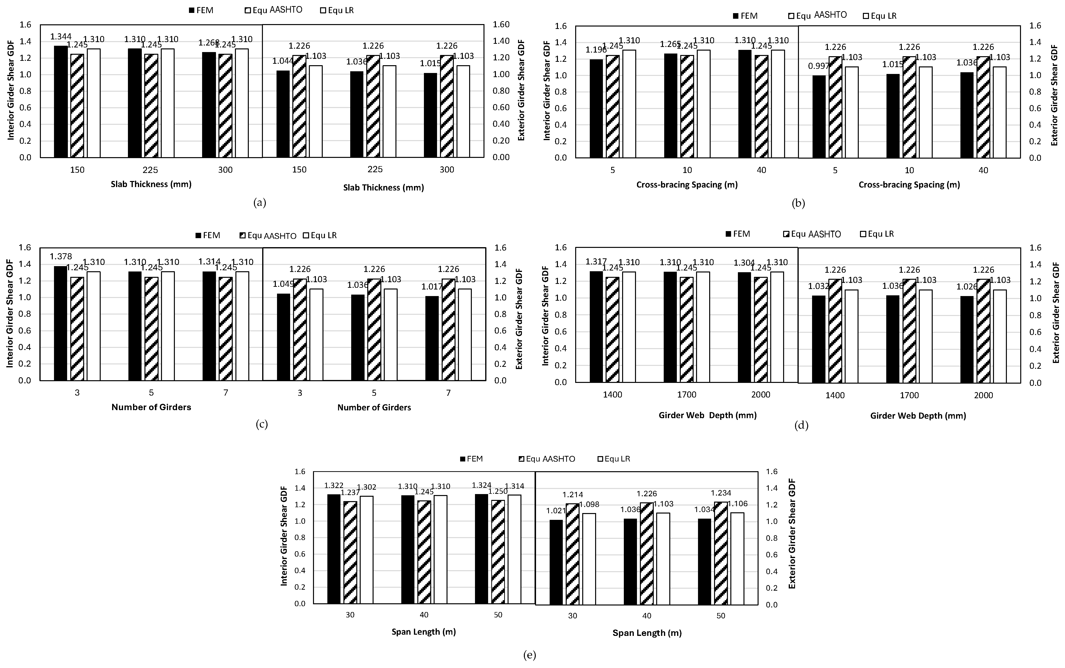
5.2. Shear in Girders Due to Live Load

In this section, the internal shear effect in the splayed girders is considered and discussed with consideration of the previously considered parameters in the flexural study, such as girder spacing, deck slab thickness, spacing of cross-bracing, number of girders, girders depth, and span length.

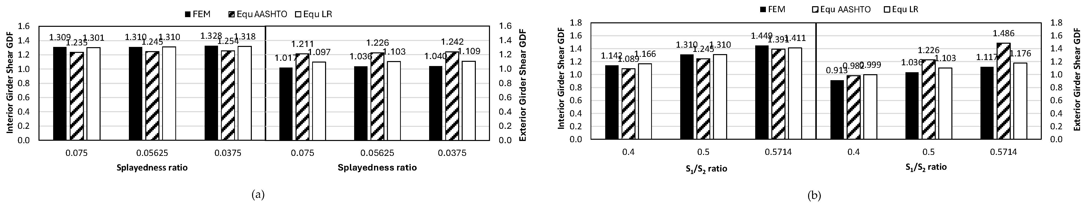
5.2.1. Effect of Girder Spacing

The shear GDF expressions in the AASHTO Bridge Design Specifications [1] only include girder spacing in the determination of the shear load effect in girders. In this study, the same bridges used to examine the flexure effect are analyzed to determine the shear effect by positioning the truck(s) longitudinally on the bridge near the support at the wider girder spacing end in order to maximize the vertical reaction under the critical girder.

Investigation of the effect of splayedness in the reference bridge B1 showed that an equivalent shear GDF based on the lever rule can be more effective in predicting the shear effect in splayed girders than using the AASHTO LRFD expressions. Therefore, the equivalent shear GDF was computed once based on the AASHTO LRFD expressions and once again based on the lever rule. Both values were then compared with the finite element model results for all fifteen bridges listed in Table 1.

The effect of the splayedness ratio (S₂ − S₁)/L is examined for the shear GDF by studying bridges B1, B2, and B3. However, since the changes in this ratio at the wide end of the bridge (the longitudinal critical position for shear) are minimal, there is almost no change in the girder spacing between the three considered bridges. This leads to insignificant changes in the finite element results of the shear GDF. Likewise, the equivalent shear GDF based on the lever rule showed negligible change between the considered bridges, as the loaded region near the end support was relatively small in comparison with the entire surface area of the bridge.

When comparing the interior girder shear GDF values computed by the three different methods, it became obvious that the AASHTO LRFD expressions yielded0 slightly lower values compared with the finite element results, while the lever rule produced almost the same outcome. For the exterior girders, the AASHTO LRFD shear GDF values were higher than the finite element results by as much as 19%, while the lever rule values were much closer to the finite element results, with a maximum difference on the conservative side equal to 7.8%.

The girder spacing ratio S₁/S₂ was also examined for the shear GDF by studying bridges B4, B1, and B5. The finite element results demonstrated that for interior girders, increasing the S₁/S₂ ratio by 14.3% resulted in a 10.54% increase in GDF value, while decreasing the S₁/S₂ ratio by 20% led to a 12.88% reduction in GDF value. The same trend was observed for the exterior girders, where increasing the S₁/S₂ ratio by 14.3% resulted in an increase in GDF value of 7.8%, while reducing the S₁/S₂ ratio by 20% resulted in an 11.86% decrease in the GDF value. It can be observed that all splayed bridges acted like regular bridges with parallel girders, in which increasing girder spacing caused a linear increase in the values of the shear GDF.

Figure 23a,b show the influence of the splayedness and girder spacing ratios on the shear GDF, respectively, for the interior and exterior girders. For bridges B1, B4, and B5, the GDF is computed based on finite element analysis, the AASHTO LRFD expressions, and the lever rule. Compared to the finite element results, the AASHTO expressions yielded slightly lower GDF values for the interior girders and up to 32.8% higher values for the exterior girders. On the other hand, using the lever rule led to reasonably close and conservative values in comparison with the refined analysis for both interior and exterior girders. Based on the outcome of the study concerning the variation in the girder spacing, the lever rule is recommended for determining the shear load effect in interior and exterior girders of splayed girder bridges in lieu of using a complex refined method.

5.2.2. Effect of Other Parameters

All the other five parameters (slab thickness, cross-bracing spacing, girder stiffness, number of girders, and span length) were investigated through the analysis of the other ten bridges, B6–B15, as shown in Table 1. As shown in Figure 24, the refined analysis demonstrated that these parameters have very minimal influence on the shear GDF values, which is an expected finding. For the shear load effect in the interior girders, the difference between the lever rule and finite element outcome ranges between −4.9% and 9.5%. The corresponding difference between the lever rule and finite element analysis for the exterior girders ranges between −0.8% and 9.4%. Compared to the finite element findings, the overall results demonstrate that the lever rule gives much more sensible results than the AASHTO LRFD shear GDF expressions for the majority of the considered cases.

5.2.3. Summary of Shear Results

The results presented in the previous sections showed that for the 15 bridges analyzed for shear, use of the lever rule yields more reasonable and slightly conservative shear GDF values than the AASHTO LRFD GDF expressions. Figure 25 compares the finite element shear GDF values with the corresponding shear GDF values based on the lever rule for both interior and exterior girders. For almost all the considered cases, the shear GDF values obtained using the lever rule were reasonably very close to the finite element analysis findings. Thus, for all practical purposes, it can be concluded that the GDF based on the lever rule is a good indicator of the live load shear effect in the main elements of splayed girder bridges.

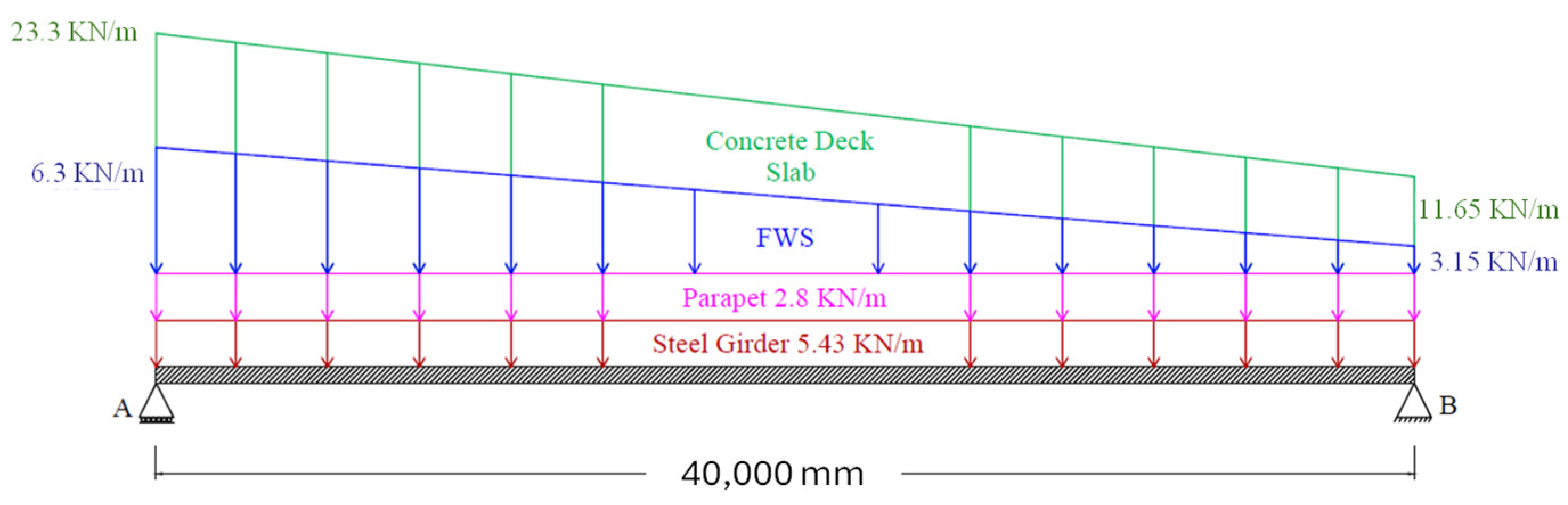
5.3. Dead Load Effect in Girders

In this study, both shored and unshored construction methods are studied and applied to the reference bridge to understand the behavior of splayed girder bridges under the influence of dead load. Finite element models are developed for both cases and the results are compared with hand calculations for the composite girder of the bridge loaded with the same dead loads based on the tributary area concept.

In shored construction, the composite girder resists all dead load components, including the girder and deck slab self-weight, parapet weight, and future wearing surface (FWS). In the analytical approach, a single composite girder of the bridge is loaded with the concrete deck slab self-weight, where the deck slab width is taken as half of the girder spacing from each side. This approach results in a linearly variable slab width along the span length equal to the girder spacing, resulting in a trapezoidal load on the composite girder. The steel girder self-weight is also represented by a uniform load along the composite girder’s length assuming the girder was supported during erection. Regarding the superimposed load from parapet weight and future wearing surface, the AASHTO LRFD Bridge Design Specifications [1] suggest distributing it equally among the girders if sufficient curing of the concrete slab has taken place. Therefore, the parapet weight is represented by a uniform load along the span and its magnitude is taken equal to the summation of parapet loads at both edges of the bridge divided by the number of girders. However, due to the bridge splayedness, the FWS load varies along the girder length, and it is represented by a trapezoidal load with a magnitude at any section equal to the total FWS load per unit width at that section divided by the number of girders. Cross-bracing, if present, is represented by point loads along the span of the composite girder; these loads vary in magnitude from one point to another based on the cross-bracing weight, where it changes due to the variable girder spacing along the span. The composite girder dead load for the reference bridge B1 is shown in Figure 26. The composite girder is then analyzed as a line element using statics, and the moment at the midspan is computed to find the elastic stress at the bottom flange of the girder in the composite section at the midspan. The ensuing stress due to analytically calculated dead load is compared with the one obtained from the finite element (FE) results at the midspan, as shown in

Table 3. Maximum tensile stress in shored composite girders of reference bridge B1 at midspan due to future wearing surface and parapet weight.

Girder	Analytical Calculation	FE Exterior Girder (G1)	FE First Interior Girder (G2)	FE Intermediate Girder (G3)
Stress (MPa)	77.77	78.57	74.51	73.44

.

It is clear from the results included in Table 3 that the stresses are very close to each other. The magnitude of the stress resulting from the analytical approach using the transformed composite girder geometric properties is greater than the corresponding stress from the finite element model by 4.2% for the first interior girder and by 5.5% for the intermediate girder, but lower by 1% for the exterior girder. This finding indicates that the analytical approach provides a reasonable approximation of the dead load effect in individual girders for the shored construction method in splayed girder bridges.

In the unshored girder construction case, the composite girder resists loads resulting from FWS and parapet weight, while the non-composite girder resists all other dead loads. Therefore, in the analytical approach, the composite girder is only loaded by the trapezoidal load representing the FWS and the uniform load representing the parapet weight, as shown in Figure 27 for reference bridge B1. Both load components are assumed to be distributed equally among the bridges’ girders, as suggested by the AASHTO LRFD specifications, and computed in the same manner as presented previously in the shored construction case. The remaining dead load due to self-weight and the weight of the concrete deck slab within the tributary width is assumed to be carried by the non-composite steel girders. Structural analysis of the bare steel girder subjected to loads on the non-composite section is not considered here since there is no interaction from other girders; hence, the analytical solution in this case would match the finite element results.

The composite girder is then analyzed, and the midspan moment and corresponding stress are computed again in the same manner as in the shored construction method. The analytical results, based on the analysis of a line element and mechanics of elastic material principles, are compared with the finite element findings at the midspan, as shown in

Table 4. Maximum tensile stress in unshored composite girders of reference bridge B1 at midspan due to future wearing surface and parapet weight.

Girder	Analytical Calculations	FE Exterior Girder (G1)	FE First Interior Girder (G2)	FE Intermediate Girder (G3)
Stress (MPa)	19.23	21.00	20.25	19.20

.

The results of the maximum tensile stress in the girders, presented in Table 4, for the case of unshored construction are close to each other. While the stress value obtained with the analytical approach is almost the same as that obtained with the finite element model for the intermediate girder, it is 5.3% lower for the first interior girder and 9.2% lower for the exterior girder. This outcome shows that distributing the dead load equally among all girders, as suggested by the AASHTO LRFD specifications, in the unshored construction method might not be that accurate for splayed girder bridges. This finding could be due to the load from the parapet weight having greater influence on the girders within its vicinity, leading to larger dead load imposed on the exterior and first interior girders than on the central girder. In any case, this dead load component on the composite girder is a relatively smaller fraction of the total dead load, which, when combined with the remaining load on the non-composite girders, will result in closer agreement between the analytical and the finite element results.

6. Conclusions and Recommendations

The results of this study on splayed girder bridges lead to the following conclusions and recommendations:

6.1. Conclusions About Flexural Effect

• The tributary width concept that is often used in practice for regular bridges is reliable for determining the flexural dead load effect on the splayed interior and exterior girders. However, the AASHTO recommendation of equally sharing the superimposed dead load among the girders is not always very accurate, as this study showed that exterior girders receive higher loads from the parapet weight than interior girders.
• Increasing the splayedness ratio leads to reductions in GDF for flexure in both interior and exterior girders. The relationship between the GDF and splayedness ratio is almost linear.
• The splayedness ratio and girder spacing ratio cannot be used as standalone indices in a splayed girder bridge without supporting them with the actual girder spacing. Therefore, to judge the magnitude of the flexural GDF of a splayed girder bridge, a splayedness parameter plus one girder spacing at a specific location within the bridge must be provided.
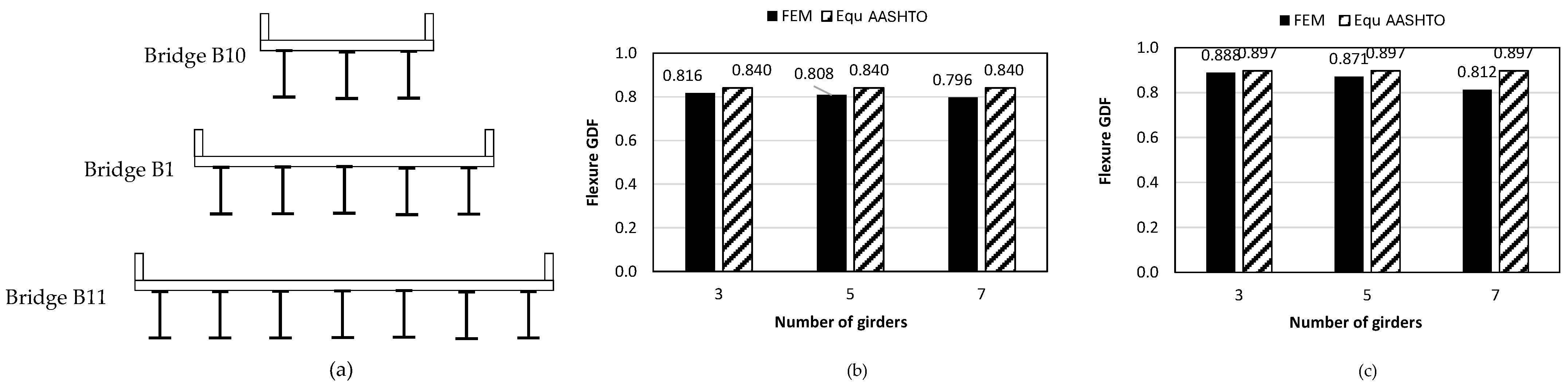
• The effect of the slab thickness on the flexural GDF for splayed girder bridges is moderate on the interior girders and negligible on the exterior girders. In addition, girder stiffness has little effect on the GDF for both interior and exterior girders. However, an increase in the number of girders beyond five can lead to some reduction in the GDF of the exterior girder, due to the possibility of rigid body rotation over the increased width of the bridge and large eccentric truck loading.
• There is a significant effect on the interior girders due to the addition of cross-bracing to splayed girder bridges, which is similar to the presence of the cross-bracing effect in regular bridges. Where the flexure GDF for interior girders dropped by more than 8% due to adding cross-bracings at 5 m spacing, it increased the exterior girder GDF by about 2%. The location of cross-bracing spacing in reference to the longitudinal truck axle positions is important, as axles directly above a cross-bracing are more equally distributed among the girders compared to axles located between cross-bracings.
• The AASHTO GDF for flexure yielded reasonable results compared to the FE models, where for the interior girders, the difference was between 2–13% on the conservative side. The high values of the flexure GDF compared with the finite element results, computed following the AASHTO specifications, were due to the presence of cross-bracing, the effect of which is not considered in the AASHTO formulas. The GDF results for exterior girders obtained using the AASHTO formulas were also very reliable, where the percentage difference was between −4% and 14% when compared with the finite element analysis outcomes. The results representing slight conservatism were recorded in bridges with extreme parameter values that exceeded the AASHTO limits.

6.2. Conclusions About Shear Load Effect

• The tributary width concept is a good approach for finding the shear dead load effect in splayed interior and exterior girders. As in the case of flexure, superimposed dead load distribution among the girders is not shared equally, as permitted by AASHTO, since exterior girders collect higher loads from the parapet weight than interior girders.
• Increasing the splayedness ratio causes a negligible effect on the GDF for shear in both interior and exterior girders. On the other hand, the increase in the smaller-to-larger girder spacing ratio, while keeping the splayedness ratio constant, results in a significant increase in the GDF for shear. As in the case of flexure, both the splayedness angle and the girder spacing ratios cannot be used as standalone indices in a splayed girder bridge without specifying the magnitude of the (smaller or larger) girder spacing.
• The effect of slab thickness on the shear GDF for splayed girder bridges is moderate in the interior girders and negligible in the exterior girders. Girder stiffness and the number of girders (if above five) have little influence on the shear GDF for both interior and exterior girders.
• Adding cross-bracing to splayed girder bridges reduces the GDF for shear in the interior girders, particularly if the cross-bracing spacing is small. The effect of using cross-bracing in splayed girder bridges on the exterior girders shear GDF is not significant since the bracing impacts these girders from one side only.
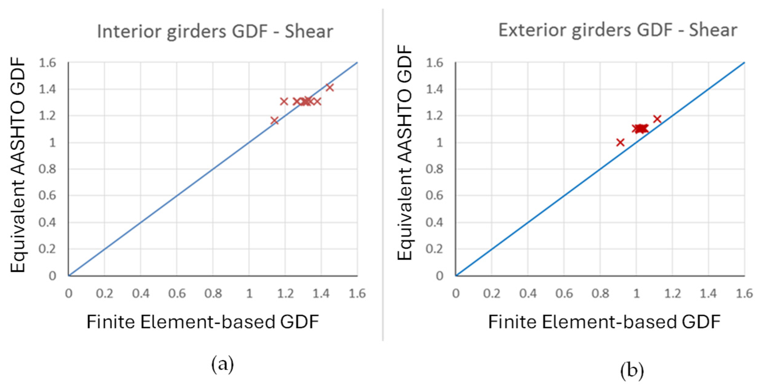
• The use of the lever rule to predict shear in interior or exterior splayed girders yields reliable results compared to the finite element outcome. Girder distribution values from the lever rule yielded results that deviated from the finite element findings by −4.9% to 9.5% for the critical interior girder and by −0.8% to 9.4% for the exterior girder. On the other hand, the AASHTO GDF for shear could not reasonably predict the shear live load effect in the girders, as the outcome from this approach yielded overly conservative values.

6.3. Recommendations

Based on the results of the finite element analysis, the AASHTO Bridge Design Specifications GDF expressions, and the lever rule, the following recommendations with regard to flexure and shear in girders that are part of splayed girder bridges can be drawn:

• The tributary width concept is a reliable approach for determining the dead load effect on the splayed interior and exterior girders. The parapet weight, when placed on the hardened concrete deck, tends to load the exterior girders more than the interior girders; hence, assuming such a load to be equally distributed among the girders is not a valid assumption.
• The girder distribution factors for flexure in the AASHTO LRFD specifications can be reasonably used for splayed girder bridges if the specific girder spacing at the location of each axle of the truck in the longitudinal direction of the bridge is considered.
• The lever rule can provide a good estimate of the live load distribution among splayed girders when subjected to shear.

References

1. AASHTO. LRFD Bridge Design Specifications, 9th ed.; American Association of State Highway and Transportation Officials: Washington, DC, USA, 2020. [Google Scholar]
2. Buckler, J.G.; Barton, F.W.; Gomez, J.P.; Massarelli, P.J.; McKeel, W.T., Jr. Effect of Girder Spacing on Bridge Deck Response; Virginia Transportation Research Council: Charlottesville, VA, USA, 2000; Final Rep., VTRC 01-R6.
3. Barr, P.J.; Amin, M.N. Shear live-load distribution factors for I-girder bridges. J. Bridge Eng. 2006, 11, 197–204. [Google Scholar] [CrossRef]
4. Tabsh, S.W.; Sahajwani, K. Approximate analysis of irregular slab-on-girder bridges. J. Bridge Eng. 1997, 2, 11–17. [Google Scholar] [CrossRef]
5. Song, S.-T.; Chai, Y.; Hida, S.E. Live-load distribution factors for concrete box-girder bridges. J. Bridge Eng. 2003, 8, 273–280. [Google Scholar] [CrossRef]
6. Puckett, J.A.; Mertz, D.; Huo, X.S.; Jablin, M.C.; Peavy, M.D.; Patrick, M.D. Simplified Live Load Distribution Factor Equations; Transportation Research Board: Washington, DC, USA, 2007; NCHRP Rep. [Google Scholar]
7. Utah Department of Transportation. Bridge Management Manual; Utah Department of Transportation: Salt Lake City, UT, USA, 2014.
8. Kansas Department of Transportation. LRFD Bridge Design; Kansas Department of Transportation: Topeka, KS, USA, 2009.
9. A. DARWin-ME, Version 1.0; American Association of Highway and Transportation Officials: Washington, DC, USA, 2011; Volume 444.
10. WSDOT. PGSuper Software 2.1 Release; BridgeSight Inc.: South Lake Tahoe, CA, USA, 2009.
11. Akbari, R.; Maalek, S. A review on the seismic behaviour of irregular bridges. Proc. Inst. Civ. Eng. Struct. Build. 2017, 171, 552–580. [Google Scholar] [CrossRef]
12. Soberón, M.C.G.; Soberón, J.M.G. Dynamic properties variation by irregular superstructure and substructure common bridges. Procedia Eng. 2017, 199, 2961–2966. [Google Scholar] [CrossRef]
13. Soleimani, F.; Mangalathu, S.; DesRoches, R. Seismic Resilience of Concrete Bridges with Flared Columns. Procedia Eng. 2017, 199, 3065–3070. [Google Scholar] [CrossRef]
14. Eom, J.; Nowak, A.S. Live load distribution for steel girder bridges. J. Bridge Eng. 2001, 6, 489–497. [Google Scholar] [CrossRef]
15. ANSYS, Version 14.0; ANSYS Inc.: Canonsburg, PA, USA, 2011.
16. Chan, T.H.; Chan, J.H. The use of eccentric beam elements in the analysis of slab-on-girder bridges. Struct. Eng. Mech. 1999, 8, 85–102. [Google Scholar] [CrossRef]
17. Barr, P.J.; Eberhard, M.O.; Stanton, J.F. Live-load distribution factors in prestressed concrete girder bridges. J. Bridge Eng. 2001, 6, 298–306. [Google Scholar] [CrossRef]
18. Hays, C., Jr.; Sessions, L.; Berry, A. Further studies on lateral load distribution using a finite element method. Transp. Res. Rec. 1986, 1072, 6–14. [Google Scholar]
19. Ventura, C.; Felber, A.; Stiemer, S. Determination of the dynamic characteristics of the Colquitz River Bridge by full-scale testing. Can. J. Civ. Eng. 1996, 23, 536–548. [Google Scholar] [CrossRef]
20. Chen, Y. Distribution of vehicular loads on bridge girders by the FEA using ADINA: Modeling, simulation, and comparison. Comput. Struct. 1999, 72, 127–139. [Google Scholar] [CrossRef]
21. Tabsh, S.W.; Tabatabai, M. Live load distribution in girder bridges subject to oversized trucks. J. Bridge Eng. 2001, 6, 9–16. [Google Scholar] [CrossRef]
22. Bishara, A.G.; Liu, M.C.; El-Ali, N.D. Wheel load distribution on simply supported skew I-beam composite bridges. J. Struct. Eng. 1993, 119, 399–419. [Google Scholar] [CrossRef]
23. Machado, M.A.; Sotelino, E.D.; Liu, J. Modeling technique for honeycomb FRP deck bridges via finite elements. J. Struct. Eng. 2008, 134, 572–580. [Google Scholar] [CrossRef]
24. Mabsout, M.E.; Tarhini, K.M.; Frederick, G.R.; Tayar, C. Finite-element analysis of steel girder highway bridges. J. Bridge Eng. 1997, 2, 83–87. [Google Scholar] [CrossRef]
25. Wu, H. Influence of Live-Load Deflections on Superstructure Performance of Slab on Steel Stringer Bridges; West Virginia University: Morgantown, WV, USA, 2003. [Google Scholar]
26. Eamon, C.D.; Nowak, A.S. Effects of edge-stiffening elements and diaphragms on bridge resistance and load distribution. J. Bridge Eng. 2002, 7, 258–266. [Google Scholar] [CrossRef]
27. Hraib, F. Finite Element Analysis of Splayed Girder Bridges. Master’s Thesis, Civil Engineering Department, American University of Sharjah, Sharjah, United Arab Emirates, June 2015. 162 pages. Available online: https://repository.aus.edu/entities/publication/92989414-e0e1-4937-b64c-20150599b82b (accessed on 1 April 2025).
28. Fang, K.I. Behavior of Ontario-Type Bridge Deck on Steel Girders. Ph.D. Thesis, Department of Civil Engineering, University of Texas at Austin, Austin, TX, USA, 1985. [Google Scholar]
29. Schonwetter, P. Field Testing and Load Rating of a Steel-Girder Highway Bridge. Master’s Thesis, Department of Civil Engineering, University of Texas at Austin, Austin, TX, USA, 1999. [Google Scholar]
30. Cai, C. Discussion on AASHTO LRFD load distribution factors for slab-on-girder bridges. Pract. Period. Struct. Des. Constr. 2005, 10, 171–176. [Google Scholar] [CrossRef]
Figure 1. Typical simply supported composite steel bridge containing flared girders.
Applsci 15 04674 g001
Figure 2. Finite element model used in the study.
Applsci 15 04674 g002
Figure 3. Properties of girders and geometry of cross-bracings: (a) girder dimensions; (b) cross-bracing configuration at the end supports and within the span.
Applsci 15 04674 g003
Figure 4. Dead load effect in the interior girder of reference bridge B1: (a) entire bridge plan; (b) single interior girder and loading; (c) shear and moment bending diagrams of interior girder.
Applsci 15 04674 g004
Figure 5. Critical longitudinal truck position in the reference bridge B1: (a) elevation; (b) plan; (c) finite element results.
Applsci 15 04674 g005
Figure 6. Critical transverse position for a single truck: (a) plan for exterior girder; (b) plan for first interior girder; (c) cross-section.
Applsci 15 04674 g006
Figure 7. Details of reference bridge B1: (a) plan; (b) cross-section; (c) finite element mesh.
Applsci 15 04674 g007
Figure 8. Load effect in reference bridge B1 by finite element analysis: (a) entire bridge; (b) normal stresses in bottom flanges; (c) shear stresses in webs.
Applsci 15 04674 g008
Figure 9. Flexural analysis of reference bridge B1: (a) transverse truck positioning; (b) GDF due to one, two and three loaded lanes.
Applsci 15 04674 g009
Figure 10. Shear GDF of reference bridge B1 due to one, two and three loaded lanes: (a) Case 1, truck lines of wheels placed parallel to parapet; (b) Case 2, truck axles placed perpendicular to girder under consideration.
Applsci 15 04674 g010
Figure 11. Alternatives to reference bridge B1: (a) bridge B1−a, exterior girder perpendicular to line of support; (b) bridge B1−b, first interior girder perpendicular to line of support.
Applsci 15 04674 g011
Figure 12. Comparison of finite element results with hand calculation for reference bridge B1: (a) flexural effect; (b) shear effect.
Applsci 15 04674 g012
Figure 13. Effect of girder splayedness ratio on flexural GDF: (a) plan of bridges B1, B2, and B3; (b) onterior girder; (c) exterior girder.
Applsci 15 04674 g013
Figure 14. Effect of girder spacing ratio on flexural GDF: (a) plan of bridges B1, B4, and B5; (b) interior girder; (c) exterior girder.
Applsci 15 04674 g014
Figure 15. Effect of the average girder spacing on flexural GDF.
Applsci 15 04674 g015
Figure 16. Effect of deck slab thickness on flexural GDF: (a) cross-section of bridges B1, B6, and B7; (b) interior girder; (c) exterior girder.
Applsci 15 04674 g016
Figure 17. Finite element-based flexural GDF as a function of the distance from the parapet for bridges B1 and B8 under two side-by-side trucks.
Applsci 15 04674 g017
Figure 18. Effect of cross-bracing spacing on flexural GDF: (a) plan of bridges B1, B8, and B9; (b) interior girder; (c) exterior girder.
Applsci 15 04674 g018
Figure 19. Effect of number of girders on flexural GDF: (a) cross-section of bridges B1, B10, and B11; (b) interior girder; (c) exterior girder.
Applsci 15 04674 g019
Figure 20. Effect of girder web depth on flexural GDF: (a) girder dimensions of bridges B1, B12, and B13; (b) interior girder; (c) exterior girder.
Applsci 15 04674 g020
Figure 21. Effect of span length on flexural GDF: (a) plan of bridges B1, B14, and B15; (b) interior girder; (c) exterior girder.
Applsci 15 04674 g021
Figure 22. Comparison between the finite element and AASHTO flexural GDF: (a) interior girder; (b) exterior girder.
Applsci 15 04674 g022
Figure 23. Effect of girder spacing on shear GDF: (a) splayedness ratio; (b) girder spacing ratio.
Applsci 15 04674 g023
Figure 24. Effect of girder spacing on shear GDF: (a) slab thickness; (b) cross-bracing spacing; (c) number of girders; (d) girder web depth; (e) span length.
Applsci 15 04674 g024
Figure 25. Comparison between the finite element and AASHTO shear GDF: (a) interior girder; (b) exterior girder.
Applsci 15 04674 g025
Figure 26. Dead load on a single composite girder of bridge B1 for the case of shored construction.
Applsci 15 04674 g026
Figure 27. Dead load on a single composite girder of bridge B1 for the case of unshored construction.
Applsci 15 04674 g027