Electric Vehicle Routing with Time Windows and Charging Stations from the Perspective of Customer Satisfaction

Abstract

The use of electric vehicles in urban transportation is increasing daily due to their energy efficiency and environmental friendliness. In last-mile logistics, route optimization must consider charging station locations while balancing operational costs and customer satisfaction. In this context, solutions for cost-oriented route optimization have been presented in the literature. On the other hand, customer satisfaction is also important for third-party logistics companies. This study discusses the Capacitated Electric Vehicle Routing Problem with Time Windows (CEVRPTW) encountered in last-mile logistics. This article defines the objective function of minimizing total tardiness and compares the routes between the service provider logistics company and the customer receiving the service. In this study, the CEVRPTW was solved for the minimum total tardiness objective function with the hybrid adaptive large neighborhood search (ALNS) algorithm. The success of ALNS was proven by comparing the differences between the optimal solutions obtained with the CPLEX Solver and the ALNS solutions. Tardiness objective function-specific operators for ALNS are proposed and supported by local search and VNS algorithms. The findings of this study contribute to the literature by analyzing the balance trade-offs between customer-oriented and cost-oriented and the effect of time windows on the number of vehicles.

1. Introduction

The increasing popularity of electric vehicles (EVs) due to environmental concerns is also increasing their use in the logistics sector day by day. With the tightening of environmental protection policies, regulations have been introduced to prevent the distribution of traditional fossil fuel vehicles in urban areas of some cities [1]. While EVs are rapidly being adopted to reduce global carbon emissions, the effects of the transformation in the transportation sector have begun to be seen and have become an important alternative to fossil fuel vehicles. This transformation is also prominent in last-mile delivery, which is all logistics activities related to delivery to customer households in urban areas. The growth of urban populations and intense e-commerce activities increase the complexity of last-mile delivery and its impact on the environment and quality of life. More and more logistics companies are adopting EVs for cargo distribution [2]. Despite the environmental benefits of EVs, their limitations, such as limited driving range and lack of charging infrastructure, continue. These problems also lead to difficulties in the route planning of EVs. Innovative solutions are needed to overcome these challenges and promote the widespread adoption of electric vehicles for last-mile delivery. These solutions should focus on improving battery technology to extend driving ranges [3], expanding charging infrastructure in urban areas [4], and implementing efficient vehicle scheduling and route planning algorithms that maximize delivery efficiency while minimizing costs [5,6,7]. Therefore, it is crucial to establish effective vehicle routing and scheduling, including operational costs, that can not only reduce total travel time but also reduce delivery costs.

Developing and implementing innovative solutions for last-mile delivery using electric vehicles is essential to address the environmental impact and logistics challenges associated with traditional fossil-fuel-based operations. Last-mile delivery has become an important need with the increasing quality of life in cities. In the increasingly competitive environment, the need for customer-satisfaction-oriented route optimization in fleet management of service providers is also obvious. Various technologies and strategies are proposed in the literature for task planning and route optimization of electric vehicles for last-mile delivery. Studies include the use of optimization algorithms, machine learning techniques, and real-time data analysis to optimize delivery routes based on factors such as traffic conditions, delivery time windows, and charging station availability [8]. By integrating these technologies and strategies, logistics companies can perform more sustainable and efficient last-mile delivery operations while reducing their carbon footprint. When the literature is examined, it is seen that studies on route optimization of electric vehicles in last-mile logistics focus on cost-oriented objectives. In the literature, it has been observed that studies that take into account the time window constraint work on cost-oriented objective functions such as minimizing total distance, total time, and total energy. It seems that there is a need for studies that take into account objective functions such as the extent to which routes meet customer constraints based on time windows, total tardiness, and the number of customer requests that cannot be met on time. These issues are of vital importance for businesses that prioritize customer satisfaction. The aim of this study is to address route optimization for customer-oriented objectives as well as cost-oriented objectives such as total travel distance and total travel time by considering charging time. The charging strategy applied in routing electric vehicles affects the total route duration, including the time the vehicle is at the charging station. In last-mile delivery, customer satisfaction is related to whether a certain product is delivered within the specified time interval. The insights and suggestions obtained with this study can guide the development of time that not only increases customer satisfaction but also reduces delivery costs by reducing total travel time and provides a win–win situation for both logistics companies and customers.

In this study, a hybrid adaptive large neighborhood search (HALNS) algorithm is proposed for the Capacitated Electric Vehicle Routing Problem with Time Windows (CEVRPTW), considering a full charging strategy in last-mile delivery. Efficient (HALNS) operators are designed to minimize tardiness by taking customer time windows into account. The proposed algorithm is tested using datasets designed for the Eskisehir Osmangazi University campus environment. To the best of our knowledge, there are no papers that address task scheduling of delivery requests by minimizing total tardiness. This paper also includes an analysis of trade-offs between the number of vehicles in the fleet and tardiness. The effectiveness of conventional cost-oriented routing and customer-oriented route optimization strategies for the last-mile delivery of electric vehicles is evaluated. The contributions of this study to the literature are summarized as follows:

• Unlike the cost-focused objective functions in the literature, the objective function of minimizing total tardiness is studied. It takes customer satisfaction into account by considering customer time windows.
• Since the ALNS operators proposed in the literature are not effective for the total tardiness objective function, new operators are proposed to serve this objective function.

The rest of this paper is organized as follows: Section 2 briefly reviews previous research on electric vehicle routing problems. The materials and methods are given in Section 3. Section 4 discusses the results and performance of the proposed system. Section 5 presents the research results and provides an outlook for future work.

2. Related Works

2.1. Studies on Capacitated Electric Vehicle Routing Problem with Time Windows

The Capacitated Electric Vehicle Routing Problem with Time Windows (CEVRPTW) is an optimization problem involving routes where an electric vehicle starts from a depot, serves customers, and then completes its route at the depot. EVs have limited load capacity, and each customer has a time window, namely “earliest start of service” and “latest start of service”. Within the time windows, each customer should be visited on the routes, and the load and charge status of the vehicles must be taken into account. In order to better analyze the studies on the EVRPTW, articles were searched for by searching the Web of Science with the keywords “Electric Vehicle Routing Problem” and “Time Windows”. The graph of the obtained articles by year is given in Figure 1.

The intense interest in this subject, especially in the last three years, can be seen in the figure. Researchers have provided comprehensive literature reviews on the subject. Among them, Erdelic and Caric (2019) analyzed EVRP variants, solution methods used in the literature, and the aspects that distinguish the studies from each other [9]. Bogyrbayeva et al. (2022) included modeling approaches and different solution methods, such as machine learning, in their research results [10]. Kalaycı and Yılmaz (2023) analyzed the historical development of the problem and solution methods in detail and showed them statistically with graphs [11].

When the literature is examined, it can be seen that studies on EVRPTW obtained routes for minimizing the total distance in the first years. In the following years, it can be seen that the majority of studies were carried out on total time minimization and total energy minimization (

Table 1. Objective functions in papers on EVRP with time windows and charging station.

Study	Minimize Total Distance	Minimize Total Time	Minimize Total Energy	Minimize Total Recharging Cost	Minimize Total Tardiness
Conrad and Figliozzi, 2011 [12]	✔	✔		✔
Schneider et al., 2014 [13]	✔
Felipe et al., 2014 [14]				✔
Goeke and Schneider, 2015 [15]	✔		✔
Hiermann et al., 2016 [16]	✔
Keskin and Çatay, 2016 [17]	✔
Barco et al., 2017 [18]			✔
Montoya et al., 2017 [19]		✔
Keskin and Çatay, 2018 [20]			✔	✔
Kancharla and Ramadurai, 2018 [21]			✔
Kancharla and Ramadurai, 2020 [22]			✔
Futelef et al., 2020 [23]		✔	✔
Bac and Erdem, 2021 [24]		✔	✔	✔
Keskin et al., 2021 [25]			✔
Zang et al., 2022 [26]			✔	✔
Erdelic and Caric, 2022 [27]	✔
Cataldo-Díaz et al., 2022 [28]		✔
Dönmez et al., 2022 [29]			✔	✔
Duan et al., 2023 [30]	✔			✔
Yu et al., 2023 [31]	✔
Xiao et al., 2023 [32]	✔
Wang et al., 2025 [33]			✔	✔
This Study	✔				✔

).

The CEVRPTW is referred to as an NP-hard combinatorial optimization problem. Pioneering studies, which also take the charging issue into consideration in CEVRPTW studies, primarily seek solutions to minimize the total distance traveled. Schneider et al. (2014) proposed a mathematical model to minimize the total distance with constraints, including a full charge strategy. They developed a new hybrid algorithm combining the modified VNS and TS methods. They tested this method with the Erdoğan and Miller (2012) dataset, proved its success, and contributed to the literature by creating new datasets [13,34]. Keskin and Çatay (2016) presented a mathematical model including partial charge strategy constraints to minimize the total distance [17]. In the following years, studies on total distance minimization have increased even more [27,30,31].

There is a need to consider the charging time when optimizing the route of electric vehicles. While calculating the route duration and the times between nodes, the waiting time at charging stations and the charging time also appear to be significant challenges in route optimization. For this reason, some researchers have included charging times in the total route duration by considering the charging station type (public, private, etc.) and charging strategies (full, partial, etc.) in electric vehicle routing and focused on minimizing the total time [19]. Bac and Erdem (2021) solved an EVRP that includes time windows, a heterogeneous fleet, and partial charging constraints with Variable Neighborhood Search (VNS) and Variable Neighborhood Descent (VND) heuristics and minimized the total time [24]. Keskin et al. (2021) addressed an important real-life problem in terms of last-mile delivery by proposing a simulation-based heuristic for waiting time optimization at charging stations [25]. Cataldo-Díaz et al. (2022) aimed to minimize the total route time, considering the time used to move between nodes in the layout, the time it takes to store battery charge at stations, and the service time at both customer locations and charging stations [28].

Minimizing the total energy consumption in electric vehicle routing is an important goal [15,20,21,22,24,25,29,33]. Range prediction or energy consumption estimation between the start and destination nodes has been widely studied in the literature. However, in route optimization within the scope of fleet management, load- and distance-dependent energy consumptions have recently been included in the model.

Some of researchers also worked on minimizing charging costs. The effects of charging speed options and charging station type (public, private) on costs, when and at which charging station the EV will charge, and even how much it will charge are also specific to EVRP issues studied in the literature [20,29,30,33].

2.2. Studies on ALNS for CEVRPTW

The CEVRPTW is solved with exact solution methods, heuristic and metaheuristic approaches, and machine learning methods. Although the methods that provide exact solutions are quite effective in small-scale problems, they cause difficulties due to excessive running time costs in large-scale problems. In machine learning methods, there are difficulties, such as data requirements and the complexity of model training processes. For this reason, metaheuristic approaches come to the fore due to their rapid applicability and flexibility. The methods used in the studies that have increased rapidly over the years are given in Figure 2.

It is seen that metaheuristics are the most preferred methods, and the ALNS algorithm is the most used metaheuristic (Figure 2). Goeke and Schneider (2015) worked with a mixed heterogeneous fleet for the problem using ALNS. They analyzed the effect of factors such as speed, slope, and load on minimizing energy consumption [15]. Keskin and Çatay (2016) studied the CEVRPTW by considering partial charge. They defined the problem mathematically and used ALNS metaheuristics to find its solution. They showed that using partial charge instead of full charge gives more efficient results [17]. Keskin and Çatay (2018) studied the problem and three different charging technologies using metaheuristics. The study compared the fleet size and energy costs with the charging speed [20]. Kancharla and Ramadurai (2018) solved the problem by minimizing the energy consumption depending on the load with the ALNS algorithm [21]. Kancharla and Ramadurai (2020) used the ALNS algorithm to solve the problem, considering nonlinear charging and load-dependent energy consumption, which allows electric vehicles to make multiple visits to charging stations [22]. Keskin et al. (2019) considered public charging stations and waiting in charging queues in dynamic situations using ALNS and Mixed Integer Linear Programming (MILP) methods [20]. Erdelić and Carić (2022) verified that the cost of a partial charging strategy is less than that of a full charging strategy with their proposed ALNS algorithm [27]. Dönmez et al. (2022) considered partial charging policies, including time windows and multiple charging technologies for mixed fleets consisting of electric and internal combustion vehicles. They calculated energy consumption and emissions by considering the load factor and optimized the cost using different charging technologies at charging stations and the partial charging policy [29]. Duan et al. (2023) used ALNS to solve the EVRPTW problem, including normal, fast, and ultra-fast charging strategies, and analyzed the cost effects of different charging technologies [30]. Yu et al. (2023) considered the electric vehicle routing problem, including time windows, partial charges, and parcel lockers. They proposed a network design based on parcel lockers and charging stations at different locations, and each customer was assigned to only one designated parcel locker. A Mixed Integer Programming (MIP) model was constructed to solve the problem, and its performance was tested using the ALNS algorithm [31]. Wang et al. (2025) considered an extended EVRPTW model, including EV delivery, self-pickup from parcel lockers (PLs), and flexible delivery methods to provide services to customers. They used the ALNS algorithm to solve the problem. They shared the results of the analysis on the effective use of parcel lockers. In the analysis, they explained that using parcel lockers can reduce customer service costs, and the cost reduction depends on factors such as customers’ locations and time windows. They also observed a decrease in the number of vehicles used in certain situations [33].

3. Materials and Methods

3.1. Problem Description

One of the most important decisions in the delivery process is the routing decisions for deliveries from the warehouse to the customers. The vehicle routing problem (VRP), first scientifically defined by Dantzig and Ramser in 1959, is the problem of determining minimum-cost routes with a fleet of vehicles to meet customer demands. The VRP, one of the problems in the NP-hard class, has many different types according to its constraints [35]. The aim of the VRP is to determine routes with minimum cost that meet all customers’ demands. There is rich scientific literature on the VRP and its many varieties, which have been studied for about 60 years [35,36,37].

A standard VRP is a vehicle routing problem with a loading capacity limit called the Capacitated Vehicle Routing Problem (CVRP). The Capacitated Electric Vehicle Routing Problem (C-EVRP) aims to plan the most suitable routes for customers by considering the energy limitations of electric vehicles and their carrying capacity constraints. Fleet operators calculate the state of charge (SoC) along the routes and plan visits to charging stations to avoid vehicles running out of charge.

The use of electric vehicles has also started to gain popularity since the mid-2000s. The demand for electric vehicles has also increased significantly with the spread of “green logistics” worldwide [38]. The use of electric vehicles, which have limitations such as limited battery life, high costs, and various charging features in today’s technology, causes distribution problems that are different from classical vehicles in fleet size and routing decisions [39]. In particular, battery charging stations are relatively few compared to classic gas stations, and the limited distances allowed by the amount of charge in the battery require that routing decisions for electric vehicles be made with special care. However, electric vehicles are becoming attractive in many different ways [40]. Studies conducted on several companies provide information about how these vehicles are used in freight distribution today. These companies implement a two-stage plan. In the first stage, loads are transported to logistics warehouse centers outside the city with fossil-fuel-burning vehicles. In the second stage, they are distributed to customers within the city using electric vehicles [41].

The EVRP, an important component of distribution systems with a significant share in logistics costs, emerges in different areas of the service sector, such as cargo transportation and automotive, food, and textile sectors where physical production occurs. The basic assumptions of the EVRP are as follows:

• The demand of each customer is known in advance, and the customer demand cannot be divided (only one vehicle can serve each customer).
• The distances between customers and between the warehouse and the customers are fixed and known in advance.
• Each vehicle has the same capacity and is ready for service in the warehouse.
• Vehicles have a specific battery capacity. The vehicles’ state of charge (SoC) should be considered in route planning.
• In the case of charging needs, a full or partial charging strategy can be applied from the charging strategies.

The Capacity and Time Window Electric Vehicle Routing Problem (CEVRPTW) is a problem that aims to optimize route planning for electric vehicles. Considering the limited battery capacities and charging times of electric vehicles, it is aimed to provide service to customers within the specified time windows. The problem includes constraints such as carrying capacity, locations of charging stations, energy consumption, charging times, and total cost (e.g., distance, time, or energy usage) and plays an important role in developing sustainable transportation solutions. A mathematical model for the Capacity Electric Vehicle Routing Problem with Time Windows (CEVRP-TW) was proposed in the literature by Schneider et al. (2014) [13]. Keskin and Çatay (2016) considered the Electric Vehicle Routing Problem as a model that allows partial charging [17]. In the study of Keskin and Çatay, situations that require vehicles to perform partial or complete charging at charging stations while carrying a specific capacity load are considered [20]. Cataldo-Díaz et al. (2022) focus on the electric vehicle routing problem and consider the batteries’ state of charge (SoC). The problem includes customers, each with a specific demand and a time window. In the proposed model, the objective function is to minimize total time, which includes travel times between nodes, the time it takes to store battery charge at stations, and the service time at both customer locations and charging stations [28]. In the Capacity and Time Window Electric Vehicle Routing Problem, minimizing the total time in the objective function is critical in increasing operational efficiency and ensuring customer satisfaction. While the limited battery capacities and charging times of electric vehicles make routing decisions more complex, time window constraints require deliveries or services to be performed within a specific time. Minimizing the total time allows vehicles to complete their tasks faster and with less energy consumption, which reduces the density at charging stations and optimizes fleet utilization, reducing costs. It also improves customer service and contributes to sustainable transportation by minimizing environmental impacts.

3.2. Proposed Adaptive Large Neighborhood Search

ALNS is a proven method in the literature for the CEVRP. Unlike the classical VRP, in this problem, where charging stations are also considered, ALNS’s destroy and repair procedures give efficient results. For this reason, we propose a hybrid adaptive large neighborhood search (ALNS) algorithm to solve the CEVRPTW while considering the full charging strategy. ALNS is a metaheuristic algorithm for solving large-scale and complex optimization problems, first introduced by Ropke and Pisinger (2006) [42]. ALNS has operators that obtain new neighbor solutions by sequentially applying structures responsible for the tasks of “destroying” and “repairing” a solution. One of the strengths of ALNS is that it allows the efficient use of operator structures and different heuristic methods. It can search the solution space more effectively with the operator selection mechanism, which increases the chance of selection of successful operators. For more detailed reviews on the acceptance criteria for ALNS, Santini et al. (2018) provide an extensive discussion [43]. Regarding the adaptive mechanism and weight update, Turkes et al. (2021) offer a comprehensive review [44]. The general framework and distinguishing aspects of these studies are examined by Mara et al. (2022), while Voigt (2024) analyzes the most commonly used and effective operators [45,46]. The pseudocode of the proposed hybrid ALNS algorithm is given in Algorithm 1.

Algorithm 1. Proposed hybrid ALNS algorithm

Input: $S^{initial}$, ${\Omega }^{-}$, ${\Omega }^{+}$, ${\Omega }^{LS}$, $N$, $K$, $Z$, $T_0$, $a$ Initialize $i, j$, $w^{+}$, $w^{-}$, $w^{LS}$, $p^{-}, p^{+}, p^{LS}$ $S^{best}$ ←$S^{initial}$, $S^{new}$ ← $S^{initial}$, $S^{current}$ ← $S^{initial}$ $T \leftarrow T_0, i \leftarrow 1, j \leftarrow 0$ repeat  if $i==0$ (mod $K$) then   Select route removal operator ${\Omega }^{-}$ using Roulette Wheel Selection   Select customer insertion operator ${\Omega }^{+}$ using Roulette Wheel Selection   $S^{new}$ ← $insert\left(remove\right(S^{current}$))  else   if $j==0$ (mod $N$) then    Select station removal operator ${\Omega }^{-}$ using Roulette Wheel Selection    Select station insertion operator ${\Omega }^{+}$ using Roulette Wheel Selection    $S^{new}$ ← $insert\left(remove\right(S^{current}$))   else    Select customer removal operator ${\Omega }^{-}$ using Roulette Wheel Selection    Select customer insertion operator ${\Omega }^{+}$ using Roulette Wheel Selection    $S^{new}$ ← $insert\left(remove\right(S^{current}$))   end if  end if  acceptance rate ← $e^{(-(f\left(S^{new}\right)-f\left(S^{current}\right))/T)}$  if f($S^{new}$) < f($S^{current}$) or acceptance rate > random(0,1) then   $S^{current}$ ← $S^{new}$   if f($S^{current}$) < f($S^{best}$) then    $S^{best}$ ← $S^{current}$   end if   $j$ ← 0  else   $j$ ← $j$ + 1  end if  if $i==0$ (mod β) then   $S^{current}$ ← Apply VNS-Based Local Search Procedure  end if  if $i==0$ (mod $Z$) then   Update $w^{+}$, $w^{-}$, $w^{LS}$ with scores $p^{-}, p^{+}, p^{LS}$  end if  $T \leftarrow T \ast \alpha$  $i \leftarrow i+1$ until stopping criteria is met; return $S^{best}$

The algorithm changes the solution with the removal and insertion operators in each iteration and creates $S^{new}$ solutions. The solution is a list of routes. The procedures for calculating the cost of a solution based on the objective function are presented in

Table 2. Example solution of an RC05 problem and calculation of the tardiness objective function.

Solution (S)	Route Detail
Route 1:	cs5	→	75	→	42B	→	cs4	→	31	→	115	→	32	→	cs5
$\mathrm{Travel} \mathrm{Time} \mathrm{Between} \mathrm{Two} \mathrm{Nodes} ({tt}_{j-1, j}$)	-	86.60	-	102.12	-	38.57	-	18.18	-	88.501	-	39.37	-	53.973	-
$\mathrm{Arrival} \mathrm{Time} \mathrm{at} \mathrm{Node} (a_j$)	0	-	86.60	-	646.12	-	807.57	-	1337.19	-	1580.501	-	1799.87	-	2033.843
$\mathrm{Service} \mathrm{Time} (s_j$)	-	-	120	-	120	-	-	-	120	-	180	-	180	-	-
$\mathrm{Charging} \mathrm{Time} ({tch}_j$)	-	-	-	-	-	-	511.427	-	-	-	-	-	-	-	-
$\mathrm{Time} \mathrm{Window} [e_j,l_j$]	-	-	[424, 487]	-	[649, 729]	-	-	-	[1372, 1448]	-	[1459, 1531]	-	[1322, 1378]	-	-
$\mathrm{Tardiness} (T_j$)	-	-	0	-	0	-	-	-	0	-	49.50	-	421.87	-	-
Total Tardiness	471.37

.

The calculation of tardiness for customer nodes is as follows:

$$\mathrm{m}\mathrm{i}\mathrm{n}\sum _{\mathrm{j}=1}^{\mathrm{n}}{\mathrm{T}}_{\mathrm{j}}\hspace{1em}\mathrm{j}\in \mathrm{C}$$

(1)

$${\mathrm{T}}_{\mathrm{j}}=\mathrm{m}\mathrm{a}\mathrm{x}\left\{0,{\mathrm{a}}_{\mathrm{j}}-{\mathrm{l}}_{\mathrm{j}}\right\}\hspace{1em}\mathrm{j}\in \mathrm{C}$$

(2)

$${\mathrm{a}}_{\mathrm{j}+1}={\mathrm{a}}_{\mathrm{j}}+{\mathrm{s}}_{\mathrm{j}}+{\mathrm{t}\mathrm{t}}_{\mathrm{j},\mathrm{j}+1}\hspace{1em}\mathrm{j}\in \mathrm{C}$$

(3)

$${\mathrm{a}}_{\mathrm{j}+1}={\mathrm{a}}_{\mathrm{j}}+{\mathrm{t}\mathrm{c}\mathrm{h}}_{\mathrm{j}}+{\mathrm{t}\mathrm{t}}_{\mathrm{j},\mathrm{j}+1}\hspace{1em}\mathrm{j}\in \mathrm{C}\mathrm{S}$$

(4)

The objective function is given in Equation (1), minimizing the total tardiness while considering customers’ time windows. $T_j$ represents the tardiness of customer node $j$. If the vehicle arrives at the customer within the time window, tardiness will be zero. Otherwise, tardiness occurs up to $T_j$ (Equation (2)). Equations (3) and (4) define the calculation of arrival time based on whether the previous node is a customer or a charging station. In Equation (3), $a_j$ is the arrival time at node $j$, $s_j$ is the service time at node $j$, $l_j$ is the latest start time to service value, and ${tt}_{j, j+1}$ is the travel time between node $j$ and node $j+1$ ($j\in C$; $C$ denotes the set of customers). In Equation (4), ${tch}_j$ represents the charging time at node $j$ ($j\in CS$; $CS$ denotes the set of charging stations).

According to the obtained cost value, new solutions are accepted using the temperature-dependent Simulated Annealing (SA) acceptance criterion. The new solutions must respect the constraint in Equation (5) regarding battery capacity.

$${\mathrm{S}\mathrm{o}\mathrm{C}}_{\mathrm{j}}>0$$

(5)

If Equation (5) is not satisfied, the new solution is rejected. ${SoC}_j$ represents the state of charge at node $j$. The updated charge level at the next node $j+1$ is calculated as shown in Equation (6), where $ecr$ represents the energy consumption rate and $d_{j, j+1}$ represents the distance between nodes $j$ and $j+1$.

$${\mathrm{S}\mathrm{o}\mathrm{C}}_{\mathrm{j}+1}={\mathrm{S}\mathrm{o}\mathrm{C}}_{\mathrm{j}}-(\mathrm{e}\mathrm{c}\mathrm{r}\times {\mathrm{d}}_{\mathrm{j},\mathrm{j}+1})$$

(6)

Then, the algorithm expands the solution space with local search (LS) methods. It continues these operations until the stopping criterion is met. In order to use the operator structures efficiently, the algorithm updates the weights $w^{-}$, $w^{+}$, $w^{Ls}$ using the $p^{-}, p^{+}, p^{LS}$ scores obtained every $Z$ iteration. Details are given in Section 3.2.1 for the initial solution, Section 3.2.2 for the neighborhood solutions, Section 3.2.3 and Section 3.2.4 for operators, and Section 3.2.5 for the LS method.

3.2.1. Initial Solution

The proposed heuristic for minimizing customer tardiness in the initial solution starts by creating the number of routes obtained by dividing the total customer demand by the vehicle load capacity. All customers are assigned to each route by sorting them according to their latest start time to service value. Customers assigned to routes are added as long as they do not exceed the vehicle capacity. The pseudocode of the initial solution is given in Algorithm 2.

Algorithm 2. The proposed heuristic algorithm for initial solution generation

Input: $customer\_list$ Sort all $customers$ by their $due\_date$ in ascending order Calculate the $total\_demand$ of customers $num\_routes \leftarrow ⌈total\_demand/vehicle\_capacity⌉$ $routes \leftarrow [ ]$ for $route$ in $num\_routes$ do   $route\left[i\right] \leftarrow [ ]$ end for $route\_index \leftarrow 1$ for $customer$ in sorted $customer\_list$ do   if adding the $customer$ to $route\left[rout{e}_{index}\right]$ does not exceed $vehicle\_capacity$ then     Append the $customer$ to $route[route\_index]$   else     $route\_index \leftarrow route\_index+1$     Append the $customer$ to the new route: $route[route\_index]$   end if end for return $routes$

3.2.2. Neighborhood Solutions

ALNS creates new solutions by destroying a solution and repairing it again. It selects and applies an operator from the ${\Omega }^{-}$ removal operator set at each step. This causes the structures on the route to be removed from the solution. Then, with the operator selected from the ${\Omega }^{+}$ insertion operator set, it inserts the removed structures back into the routes with specific approaches. Thus, a new solution is obtained, and neighboring solutions are discovered. The selection of an operator $i$ depends on the probability $w\left(i\right)/\sum _{i’\in {\Omega }_{+,-}}w{(i}^{’})$. This probability is calculated depending on each operator’s weight $\left(w\right).$ Initially, the weights of all operator groups are equal; ${\displaystyle \frac{1}{{\Omega }_{+}}}$ gives the weight of insertion, and ${\displaystyle \frac{1}{{\Omega }_{-}}}$ gives the weight of the removal operators. Roulette wheel selection is used to select the operators. Within the operator group, the weight of each operator is calculated, and the probability of using the operator with the higher weight increases. This increase is calculated according to the state of the newly obtained solution $S^{new}$, as given in Equation (7).

$${\pi }_{\mathrm{i}}=\left\{\begin{array}{c}{\pi }_1, \mathrm{if} {\mathrm{S}}^{\mathrm{n}\mathrm{e}\mathrm{w}}<{\mathrm{S}}^{\mathrm{b}\mathrm{e}\mathrm{s}\mathrm{t}} \hfill \\ {\pi }_2, \mathrm{if} {\mathrm{S}}^{\mathrm{b}\mathrm{e}\mathrm{s}\mathrm{t}}<{\mathrm{S}}^{\mathrm{n}\mathrm{e}\mathrm{w}}<{\mathrm{S}}^{\mathrm{c}\mathrm{u}\mathrm{r}\mathrm{r}\mathrm{e}\mathrm{n}\mathrm{t}}\hfill \\ {\pi }_3, \mathrm{if} {\mathrm{S}}^{\mathrm{n}\mathrm{e}\mathrm{w}} > {\mathrm{S}}^{\mathrm{c}\mathrm{u}\mathrm{r}\mathrm{r}\mathrm{e}\mathrm{n}\mathrm{t}}\hfill \\ 0 , \mathrm{if} {\mathrm{S}}^{\mathrm{n}\mathrm{e}\mathrm{w}}=\varnothing \end{array}\right.$$

(7)

${\pi }_1$, ${\pi }_2$, and ${\pi }_3$ are obtained based on how good the new solution is. The score is ${\pi }_1$ if the applied values are the operators that led to the best solution, ${\pi }_2$ if they improved the existing solution, ${\pi }_3$ if it is an acceptable solution, and zero if no solution was found. At iteration step Z at the specified iteration lifting frequency, the operator weights are updated with Equation (8).

$$\mathrm{w}(i’)=\left\{\begin{array}{c}\begin{array}{c}(1-\mathrm{r})·\mathrm{w}\left(i\right)+\mathrm{r} · {\pi }_i/{\mathrm{Q}}_i\hspace{1em}, \mathrm{if} {\mathrm{Q}}_i>0 \\ (1-\mathrm{r})·\mathrm{w}\left(i\right) , \mathrm{if} {\mathrm{Q}}_i=0\end{array}\end{array}\right.$$

(8)

When updating the weight, the previous weight value $w\left(i\right)$, the number of times operator $i$ is used $Q_i$, and the total score of operator $i$ are used. $r$ is a parameter in the interval (0, 1) and determines whether the score or the old value dominates when determining the new value.

3.2.3. Removal Operators

Removal operators are important for obtaining different neighborhoods. Examining the existing structures in the routes breaks the solution in certain situations and provides the opportunity to create better routes. This study uses three groups of removal operators: customer, charging station, and route.

Customer Operators: Customer removal operators aim to remove customers from the route. When the operators are applied, the customers removed from the solution are added to the unserved customer list and removed from the served customer list. When the operators are applied, the number of customers to be removed $\left(P\right)$ is set as $min\left(\right[0.4TC, 60\left]\right)$ of the total number of customers $\left(TC\right)$ [21]. In addition to the well-known operators Random-Customer Removal, Related-Customer Removal, and Worst-Distance-Customer Removal, we propose three more operators. Random-Customer Removal implements the removal of $P$ customers randomly selected from a list of all customers from the relevant routes. Related-Customer Removal takes a seed customer selected from the list of all customers as a reference and calculates the distance of all other customers to this customer as a cost. It removes the P lowest cost customers from the related routes. The purpose of this operator is to remove clustered customers that are close to each other. Worst-Distance-Customer Removal, on the other hand, is cost-oriented and calculates how much distance cost all the customers on all routes incur in the solution and removes the P customers that increase the cost the most for the solution. These operators are commonly used heuristics in the literature [42,46,47]. In addition, the following operators are proposed in this study:

• Tardiness versus Worst-Distance-Customer Removal: The proposed operator evaluates the cost impact of each customer across all routes by considering both their earliest service start time and their distance from the preceding node. The objective is to identify and remove the customer $P$ whose presence contributes the most to increased route costs. By eliminating customers with late service start times from the beginning of a route, this approach enhances schedule efficiency and minimizes overall tardiness. The pseudocode is given in Algorithm 3.

Algorithm 3. Tardiness versus Worst-Distance-Customer Removal

Input: $served customers, unserved customers, routes$ $P\leftarrow$ the number of customers to be removed from the solution $customers\_to\_remove\leftarrow \left[\right]$ for each $route$ in $routes$ do   for each $node$ in $route$ do     if $node$ is Customer then       $before\_node$ ← Find before node       $cost$ ← $node.earliest\_start\_time\_to\_service \times distance from before\_node to node$       Append (node, cost) to $customers\_to\_remove$     end if   end for end for $sorted\_customer$ ← Sort $customers\_to\_remove$ by cost descending $customers\_to\_remove$ ← $sorted\_customer[0:P]$ Remove every $customer$ in $customers\_to\_remove$ Update $served customers$and $unserved customers$

The cost function is formulated by considering both distance and time windows. The cost, ${earliest\_start\_time\_to\_service}_{j+1}\times {distance}_{j, j+1}$ (j represents nodes), enables a better balance between geographical and time constraints. Since both distance and tardiness are to be minimized, multiplication is a suitable form. If one component was to be minimized and the other maximized, a ratio might have been more appropriate.

2.

Tank-Capacity-Violation-Customer Removal: Unlike other removal strategies, the operator targets inconvenient routes requiring charging stations. It removes the first node and all subsequent nodes from the solution on routes where the vehicle cannot complete its route within the available battery capacity. The goal is to optimize charging efficiency by shortening routes that require charging and eliminating unnecessary charging station visits. This results in more efficient energy use and improves overall route feasibility. The pseudocode is given in Algorithm 4.

Algorithm 4. Tank-Capacity-Violation-Customer Removal

Input: $served customers$, $unserved customers$, $routes$ for each $route$ in routes do   if tank capacity violation on the route then     $node$ ← Find node where SoC is negative     if $node$ == $route[-1]$ then       $last\_customer$ ← Get $last\_customer$ in route       Remove $last\_customer$     else       $node\_index$ ← Get index       Remove $route[node\_index:-1]$     end if   end if end for Update $served customers$ and $unserved customers$

3.

Time-Window-Violation-Customer Removal: The operator targets infeasible routes where time window constraints are violated. It identifies the first overdue customer and removes both that customer and all subsequent customers from the route. The goal is to improve the feasibility and efficiency of the overall route plan by reconfiguring routes to ensure compliance with time window constraints. Eliminating delayed customer sequences improves compliance with service time requirements and helps minimize overall tardiness. The pseudocode is given in Algorithm 5.

Algorithm 5. Time-Window-Violation-Customer Removal

Input: $served customers$, $unserved customers$, $routes$ for each $route$ in $routes$ do   if time window violation on the $route$ then     $node$ ← Find node where time window violation     if $node$ == $route[-1]$ then       $last\_customer$ ← Get $last\_customer$ in $route$       Remove $last\_customer$     else       $node\_index$ ← Get index       Remove $route[node\_index:-1]$     end if   end if end for Update $served customers$ and $unserved customers$

Route Operators: Route removal operators remove selected routes from the solution with certain approximations. This process is applied every $K$ iteration instead of every iteration due to runtime cost. The number of routes to be removed $\left(W\right)$ is determined in the range of $min(0.1TR, 0.4TR)$ depending on the total number of routes $\left(TR\right)$ [21]. Random-Route Removal and Greedy-Route Removal operators are used in the literature. Random-Route Removal removes $W$ randomly selected routes from all routes in the solution [48]. Greedy-Route Removal removes the $W$ routes with the lowest number of customers. Its purpose is to create balanced routes in terms of the number of customers and to prevent routes with a small number of customers from being included in the solution [17]. In addition to these operators, we propose two more operators focused on tardiness and infeasibility in this study.

• Max-Tardiness-Route Removal: The proposed operator examines each of the routes in the solution and calculates their tardiness. It sums up the total tardiness on a route and keeps the tardiness on the route as costs. It removes the $W$ routes with the highest tardiness from the solution. The pseudocode is given in Algorithm 6.

Algorithm 6. Max-Tardiness-Route Removal

Input: $served customers, unserved customers, routes$ W ← Calculate number of routes to be removed from the solution $routes\_to\_remove$ ← [ ] for each $route$ in $routes$ do   $cost$ ← Calculate total tardiness of the $route$   Append ($route$, $cost$) to $routes\_to\_remove$ end for $sorted\_routes$ ← Sort $routes\_to\_remove$ by cost descending $routes\_to\_remove$ ← $sorted\_routes[ 0 : W ]$ Remove every route in $routes\_to\_remove$ Update $served customers$ and $unserved customers$

2.

Infeasible-Route Removal: The proposed operator examines each of the routes in the solution in terms of state of charge status, load capacity, and time window. It removes $W$ infeasible routes from the solution. This operator paves the way for the deconstruction of infeasible solutions. The pseudocode is given in Algorithm 7.

Algorithm 7. Infeasible-Route Removal

Input: $served customers, unserved customers, routes$ W ← Calculate number of routes to be removed from the solution $routes\_to\_remove$ ← [ ] for each $route$ in $routes$ do   if $route$ is not feasible by (tank capacity, payload capacity time window) then     Append $route$ to $routes\_to\_remove$   end if end for $routes\_to\_remove$ ← $routes\_to\_remove[0:W]$ Remove every $route$ in $routes\_to\_remove$ Update $served customers$ and $unserved customers$

Station Operators: Charging station removal operators remove selected stations from the solution with certain approximations. Instead of every iteration, the process is applied once in N iterations, where no improvement occurs. The number of stations to be removed $\left(Q\right)$ is set as $min(0.1TS, 10)$ of the total number of charging stations $\left(TS\right)$ [21]. Two station removal operators were used in this study. Random-Station Removal removes $Q$ randomly selected stations from the list of stations on all routes in the solution. Worst-Charge-Usage-Station Removal examines the routes with stations in the solution. It calculates the remaining charge when arriving at the station and takes it as a cost. The $Q$ stations with the highest cost are removed from the relevant routes. This operator aims to prevent going to the station when the remaining charge is high.

3.2.4. Insertion Operators

Insertion operators play a role in re-incorporating nodes previously removed from routes back into solutions. These operators edit and optimize routes while adhering to problem constraints such as time windows, vehicle capacity, and charging requirements to ensure the solution remains viable. In this study, two different groups of insertion operators are used: customer and charging station.

Customer operators: These operators insert the customers that are removed from the routes and added to the unserved customer list back to the routes. It is important that the customers to be included in the routes can be inserted into feasible locations. There are three commonly used operators in the literature, namely Random-Customer Insertion, Greedy-Customer Insertion, and Regret-2-Customer Insertion. Random-Customer Insertion tries to include each customer in the unserved customer list by selecting a random route and a random location in the solution [49]. However, in this study, the route arrangements of the operators do not allow the routes to exceed the vehicle capacity. Greedy-Customer Insertion examines each customer in the unserved customer list in order and inserts the customer with the least insertion cost among all routes. Regret-2-Customer Insertion calculates the best insertion and second-best insertion costs for each customer in the unserved customer list. The cost between these two values is determined as the regret value. The customer with the highest regret value is selected and added to the appropriate location. The purpose of this operator is to reduce the cost increase in future insertions and to prevent the cost increase caused by greedy approaches [47]. In addition to these operators, we propose three more operators that minimize the distance cost while adapting to customer time windows.

• Best-Customer Insertion: The proposed operator examines all routes for each customer in the unserved customer list. For all locations in the routes, the distance to the customer to be added multiplied by the earliest start time to service value is taken as the cost. If the current location is a station or a warehouse, the cost is calculated by taking the nearest customer’s earliest start time to service value. This operator aims to ensure not only distance cost but also time window compatibility in the current route. The pseudocode is given in Algorithm 8.

Algorithm 8. Best-Customer Insertion

Input: $served customers, unserved customers, routes$ $customer\_to\_added\_new\_route$ ← [ ] $customer\_cost$ ← [ ] for each $unserved customer$ in $unserved customers$ do   for $route$ in $routes$ do     for $node$ in $route$ do       if $node$ is Customer then         $before\_node$ ← Find before node         $distance$ ← Calculate distance from $before\_node$ to              $unserve{d}_{customer}$         cost ← $node.earliest\_start\_time\_to\_service\times distance$         if not payload capacity violation then           Append $(node, cost, position)$ to $customer\_cost$         end if       end if     end for   end for   if $customer\_cost$ != [ ] then     Append every $customer$ in $customer\_cost$ at position   else     Append $unserved\_customer$ to $customer\_to\_added\_new\_route$   end if end for while $customer\_to\_added\_new\_route$ != [ ] do   $new\_route$ ← [ ]   Append every $customer$ in $customer\_to\_added\_new\_route$ while payload-capacity violation end while Update $served customers$ and $unserved customers$

2.

Time-Window-Greedy-Customer Insertion: Following the time window constraints, the proposed operator inserts each unserved customer into the first available position in the routes. The insertion decision is made by evaluating the latest start time to service $\left(l_i\right)$ value of customer i and the travel time $\left(t_{ij }\right)$ between customers $i$ and $j$. A feasible insertion is determined based on the condition $(l_i + t_{ij }< l_j)$. Thus, instead of only considering the latest start time to service value, the travel time is also considered to obtain a suitable time window. The pseudocode is given in Algorithm 9.

Algorithm 9. Time-Window-Greedy-Customer Insertion

Input: $served customers, unserved customers, routes$ for each $unserved customer$ in $unserved customers$ do   for $route$ in $routes$ do     for $node$ in $route$ do       if $node$ is Customer then         $travel\_time$ ← Calculate travel time between $unserved\_customer$ and $node$         if ($unserved\_customer. latest\_start\_time\_to\_service+travel\_time$) $<$ $node.due\_date$ then           Insert $unserved\_customer$ into $route$ at position of $node$         end if       end if     end for   end for end for Update $served customers$ and $unserved\_customers$

3.

Time-Window-Feasible-Customer Insertion: The proposed operator differs from the Time-Window-Greedy-Customer Insertion by first reordering the unserved customers based on their latest start time to service value. After sorting, the operator evaluates all feasible insertion positions across the available routes. The insertion process ensures that the updated route remains feasible in terms of both time window constraints and vehicle load capacity. The pseudocode is given in Algorithm 10.

Algorithm 10: Time-Window-Feasible-Customer Insertion

Input: $served customers, unserved customers, routes$ $customer\_to\_added\_new\_route$ ← [ ] $unserved\_customers$ ← Sort $unserved customers$ by latest start time to service for each $unserved\_customer$ in $unserved\_customers$ do   for $route$ in $routes$ do     Find the $best\_position$ cost of $unserved\_customer$ into every position of route     if $best\_position$ == [ ] then       Append $unserved\_customer$ to $customer\_to\_added\_new\_route$     else       Insert $unserved\_customer$ to $best\_position$     end if   end for end for while $customer\_to\_added\_new\_route$ != [ ] do   $new\_route$ ← [ ]   Append every $customer$ in $customer\_to\_added\_new\_route$ while payload capacity violation end while Update $served customers$ and $unserved customers$

Station Operators: Including charging stations in routes is important in EVRPs and considerably increases the problem’s difficulty. The station insertion operators used in this study only add routes that are infeasible due to charging constraints and whose SoC level will be insufficient. The stations added to the routes bring extra time costs due to the use of the full charging strategy. Therefore, it is important to add stations in appropriate locations. Three station insertion operators were used in this study. Random-Nearest-Station Insertion inserts the charging station closest to the random points of the routes with an insufficient SoC level. Greedy-Station Insertion calculates the first node where the charging level will be negative in routes with an insufficient SoC level and adds the closest station before this node. Best-Station Insertion scans the route backward, starting from the node where the charging level will be negative for routes with an insufficient SoC. It calculates the closest charging station to each appropriate point by looking at the cost $d_{i,station }+ d_{station, j}$. It inserts the charging station with the lowest cost that will make the route feasible. This operator adds not only the cost of traveling from one point to the station but also the cost of traveling from the station to the next point.

3.2.5. Local Search

Local search (LS) methods were included in this study due to their fast applicability and ability to produce effective solutions, and their aim was to search the solution space faster. In order to apply LS methods, the VNS-based procedure was used [13,50,51]. The pseudocode is given in Algorithm 11.

Algorithm 11. VNS-based LS

Input: $S^{current}$, $k_{max}$ $k$ $\leftarrow 1$ while $k$ $\le$ $k_{max}$ do   Select LS operator ${\Omega }^{LS}$ using Roulette Wheel Selection   $S^{new}$← Local_Search($S^{current}$)   if f($S^{new}$) < f($S^{current}$) then     $S^{current}$ ← $S^{new}$     $k$ ← 1   else     $k$ ← $k$ + 1   end if end while return $S^{current}$

Two groups of LS methods are used for the problem: intra-route (Intra) and inter-route (Inter) [9,27]. In IntraRelocate, a customer selected from a route is moved to another location on the same route. This process aims to reduce the cost of a single route. In IntraExchange, the locations of two customers selected on a route are swapped. In IntraOrOpt, a consecutive customer segment selected on a route is moved to another location. It can be considered the relocation of a customer group within a route. In IntraTwoOpt, two customer arcs selected on a route are arranged in reverse on the route. InterRelocate is the process of moving a customer selected on a route to a different route. InterExchange is the process of swapping customers selected from two different routes with each other. InterCrossExchange is the mutual relocation of customer segments selected from two different routes. Inter2Opt* is the process of swapping customer segments selected on two different routes crosswise on the routes.

4. Experimental Results

4.1. Validation of the Adaptive Large Neighborhood Search

The CEVRPTW dataset containing the Eskişehir Osmangazi University campus environment data is used in this study [52,53]. For instance, the RC05 test problem with five customers is given in

Table 3. RC05 test problem.

Customer ID	Location	Earliest Start Time to Service	Latest Start Time to Service	Service Time	Request
75	39.747233–30.47377	424	487	120	38
42B	39.752333–30.481199	649	729	120	95
32	39.752487–30.488123	1322	1378	180	76
31	39.752941–30.483072	1372	1448	120	57
115	39.752373–30.490197	1459	1531	180	76

.

The map of the ESOGU environment, which represents customers, charging stations, and warehouses in the datasets, is given in Figure 3.

Test problems were solved in Python 3.12 on a Windows 10 PC with an AMD Ryzen 7 4700 U @2.00 GHz processor and 8 GB RAM. The vehicle parameters were an energy consumption rate of 1.0, a charging rate of 0.18, a battery capacity of 3000 kWs, a speed of 12.5 m/s, and a load capacity of 350 kg. For large-size problems, the algorithm parameters were chosen as an iteration number of 8000, a cooling rate of 0.9980, an initial temperature of 10,000, a number of iterations without improvement (N) of 8, a number of route removal frequency (K) of 25, and a weight update frequency (Z) of 10. For small problems (5–10–20), the solution was obtained with 1000 iterations while keeping the other parameters the same. Each test problem was solved 10 times by ALNS, and the best results obtained were tabulated. In addition, optimal results were obtained using CPLEX Solver for the objective function of minimizing the total distance by using a full charging strategy. Exact solutions with zero tardiness are compared with solutions obtained by ALNS in

Table 4. CPLEX vs. ALNS results for min. total distance with time windows in small instances.

Instances	CPLEX				Proposed Hybrid ALNS				Δ%
	# of Route	Total Distance (m)	Total Tardiness (s)	Runtime (s)	# of Route	Total Distance (m)	Total Tardiness (s)	Runtime (s)
C05	2	5005.43	0	0.05	2	5005.43	0	0.198	0
R05	3	5726.1	0	0.12	3	5726.1	0	0.201	0
RC05	4	7093.17	0	0.05	4	7093.17	0	0.252	0
C10	3	7530.96	0	0.23	3	7530.96	0	0.265	0
R10	3	6823.93	0	0.06	3	6823.93	0	0.288	0
RC10	3	7349,86	0	0.19	3	7349.86	0	0.272	0
C20	6	12,736.51	0	0.44	6	12,736.51	0	3.123	0
R20	6	14,023.35	0	4.51	6	14,023.35	0	3.035	0
RC20	6	12,447.92	0	0.36	6	12,447.92	0	2.708	0
C40	11	21,145.80	0	3.41	11	21,828.27	0	17.160	3.22%
R40	11	26,316.81	0	75.09	11	27,193.94	0	16.397	3.33%
RC40	11	23,372.91	0	19.31	10	23,931.24	0	17.838	2.38%
C60	13	28,711.04 *	0	10,800	12	26,769.65	0	71.939	−6.76%
R60	12	29,396.37 *	0	10,800	12	27,550.95	0	77.537	−6.27%
RC60	12	30,000.09 *	0	10,800	12	28,464.34	0	71.303	−5.11%

* It is not the optimal solution. In large-scale problems, the mathematical model could not provide solutions in a reasonable time. The results were obtained by CPLEX in a three-hour time limit.

. In large-scale problems with 60 customers, the mathematical model could not provide solutions in a reasonable time. The results were obtained by CPLEX in a three-hour time limit.

It is seen that the proposed hybrid ALNS algorithm gives optimal solutions for up to 40 customers. For problems with 40 customers, ALNS deviates from the optimal results by 3.22%, 3.33%, and 2.38%, respectively. In test problems with 60 customers, ALNS outperforms in reasonable times, achieving distance savings of up to 6.76%. As the problem size increases, the running time of CPLEX increases significantly, while ALNS finds solutions in as little as 70 s, even for problems with 60 customers. The success of the hybrid ALNS algorithm is proven.

4.2. Trade-Offs Between Cost-Oriented and Customer-Oriented Solutions

An example route representation of the C20 problem from the obtained results is given in Figure 4.

In this study, customer-oriented and cost-oriented scenarios were created in terms of last-mile delivery. In the cost-oriented scenario, the logistics provider tries to minimize the cost by minimizing the total distance without taking into account when the customer wants the product. Classical ALNS solves the problems with operators known in the literature for the cost-oriented scenario. In the second scenario, the customer-satisfaction-oriented scenario, the aim is to optimize the route to provide customer time windows, taking into account customer satisfaction rather than cost. In this context, the number of vehicles is expected to increase. In

Table 5. Comparisons of total distances for solutions with cost-oriented and customer-satisfaction-oriented distance comparison.

Instances	Cost-Oriented Solutions				Customer-Satisfaction-Oriented Solutions				Δ%
	# of Route	Total Distance (m)	Total Tardiness (s)	Runtime (s)	# of Route	Total Distance (m)	Total Tardiness (s)	Runtime (s)
C05	2	3956.43	3423.137	0.177	2	5005.43	0	0.198	26.51
R05	2	5064.28	2652.562	0.180	3	5726.1	0	0.201	13.06
RC05	1	4956.02	4388.143	0.221	4	7093.17	0	0.252	43.12
C10	2	5645.72	6744.392	0.228	3	7530.96	0	0.265	33.39
R10	2	4980.35	7014.425	0.254	3	6823.93	0	0.288	37.02
RC10	2	5842.88	5013.898	0.244	3	7349.86	0	0.272	25.79
C20	4	9332.26	8005.543	2.801	6	12,736.51	0	3.123	36.48
R20	4	9975.22	11,432.066	2.631	6	14,023.35	0	3.035	40.58
RC20	4	9401	10,434.282	2.437	6	12,447.92	0	2.708	32.41
C40	7	15,634.88	20,972.411	12.213	11	21,828.27	0	17.160	39.61
R40	8	18,362.61	23,123.101	11,758	11	27,193.94	0	16.397	48.09
RC40	7	16,796.03	27,070.676	13,054	10	23,931.24	0	17.838	42.48
C60	11	25,095.65	2342.656	28.446	12	26,075.12	0	71.939	6.67
R60	10	26,198.41	3195.702	34.346	12	27,550.95	0	77.537	5.16
RC60	11	25,957.16	6182.938	32.952	12	28,613.43	0	71.303	9.66

, the results of our proposed hybrid ALNS for both scenarios are given, and the results are compared in terms of distance and tardiness.

The results show that the cost-driven solution has lower total distance costs; however, customer time window constraints are not met. Delays are higher compared to solutions where the total tardiness is minimized. On the other hand, in customer-satisfaction-oriented solutions, all customer time windows are met. However, in these problems, the distance cost increased by up to 50%. In order to meet customer time windows, the number of routes, and therefore, the number of vehicles, increased in the test problems except for C05. For example, in the C40 test problem, the results of the two scenarios are compared in terms of the number of routes (number of vehicles) and customer expectations (Figure 5). When customer satisfaction is not prioritized, fewer routes are created, and the vehicles’ capacities are used as much as possible. When customer satisfaction is prioritized, vehicle capacities are not fully used.

As shown in Figure 5, while distribution is performed with 7 vehicles in the cost-oriented solution, it is carried out with 11 vehicles in the customer-satisfaction-oriented solution. The vehicle occupancy rate is 91.5% in distributions with seven vehicles in the cost-oriented solution. In the customer-oriented solution, on the other hand, it is seen that half of the vehicles (58.2%) are delivered empty in the deliveries made with 11 vehicles. In this direction, it is clear that the vehicle, driver, and operational costs of the logistics provider will increase.

A comparison of the solutions of both scenarios for the R05 test problem is presented in the video [54]. Maps of the solutions in the scenarios are given in Figure 6 and Figure 7.

The cost-oriented solution is obtained by minimizing the total distance. In Scenario 1, customers are served with two vehicles.

In scenario 2, the customer-oriented solution is to increase the number of vehicles to three to meet the time windows of the customers. In the first scenario, the total tardiness is 2652.56 s, while in the second scenario, it was 0 s.

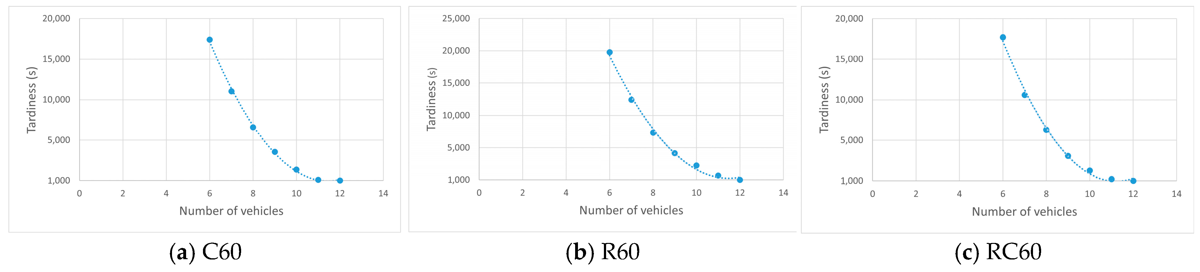
4.3. Evaluation Perspective from Fleet Management

A business may not always have as many vehicles as the number of routes required to ensure customer satisfaction. Ensuring minimum tardiness with fewer vehicles is important to decrease costs and satisfy customer time windows. Total tardiness according to fleet size scenarios is analyzed for the problems with 40 and 60 customers and given in

Table 6. Number of tardy deliveries in problems with 40 customers.

Test Problems	# of Routes	# of Vehicles	# of Tardy Deliveries	Total Tardiness (s)
C40	11	11	0	0
C40	11	10	2	1095.15
C40	11	9	7	2874.56
C40	11	8	10	5712.73
C40	11	7	13	9236.65
C40	11	6	17	14,240.29
R40	11	11	0	0
R40	11	10	2	804.75
R40	11	9	5	3424.78
R40	11	8	9	7390.73
R40	11	7	13	12,823.69
R40	11	6	17	19,573.68
RC40	10	10	0	0
RC40	10	9	2	1213.66
RC40	10	8	7	3883.94
RC40	10	7	9	8276.91
RC40	10	6	16	13,543.13

and

Table 7. Number of tardy deliveries in problems with 60 customers.

Test Problems	# of Routes	# of Vehicles	Tardy Deliveries	Total Tardiness (s)
C60	12	12	0	0
C60	12	11	1	225.94
C60	12	10	4	1272.41
C60	12	9	8	3080.85
C60	12	8	14	6265.13
C60	12	7	23	10,587.50
C60	12	6	27	17,708.64
R60	12	12	0	0
R60	12	11	2	673.87
R60	12	10	6	2265.83
R60	12	9	10	4163.19
R60	12	8	18	7337.46
R60	12	7	20	12,431.94
R60	12	6	28	19,758.54
RC60	12	12	0	0
RC60	12	11	1	91.79
RC60	12	10	5	1352.66
RC60	12	9	10	3543.19
RC60	12	8	15	6589.23
RC60	12	7	21	11,045.43
RC60	12	6	27	17,407.87

.

The results show that total tardiness increases rapidly as the number of vehicles decreases. Additional analyses were conducted to assess the statistical significance of this trend. The following hypotheses were formulated:

${\mathbf{H}}_0$: 

There is no relationship between fleet size and total tardiness.

${\mathbf{H}}_{\mathbf{a}}$: 

There is a relationship between fleet size and total tardiness.

In response to these hypotheses, the regression statistics and coefficient values for the relationship between fleet size and total tardiness are presented in

Table 8. Statistical relationship between fleet size and number of tardy deliveries for the 60-customer problems.

Regression Statistic	Value
Multiple R	0.980593
R Square	0.961563
Adjusted R Square	0.95954
Standard Error	1.991838
Observations	21

and

Table 9. Regression coefficients for the relationship between fleet size and tardy deliveries in the 60-customer problem set.

	Coefficients	Standard Error	t Stat	p-Value
Intercept	54.07143	2.003659	26.98634	1.29 × 10−16
# of Vehicles	−4.7381	0.217327	−21.8017	6.6 × 10−15

, respectively.

Table 8 shows the basic statistics of the regression analysis for the problem sets with 60 customers (R60, C60, and RC60). The high R² value (0.9616) indicates that the model explains a high proportion of the variability in the dependent variable (number of tardy deliveries). This means that 96.16% of the variation in the number of tardy deliveries can be explained by fleet size. The p-value < 0.05 confirms that there is a statistically significant relationship between fleet size and tardiness.

Table 9 shows the coefficients of the regression model that examines the effect of fleet size on the number of tardy deliveries. The coefficient for the number of vehicles is −4.7381, which implies that each additional vehicle reduces the number of tardy deliveries by 4.74 units on average. The p-value is quite low, which implies that the effect is statistically significant.

Table 10. ANOVA results for the regression model between fleet size and number of tardy deliveries in the 60-customer problem set.

	df	SS	MS	F	Significance F
Regression	1	1885.762	1885.762	475.3121	6.6 × 10−15
Residual	19	75.38095	3.967419
Total	20	1961.143

presents the ANOVA results that assess the significance of the regression model.

In Table 10, the F-statistic is quite high at 475.31, indicating that the model explains a large and significant portion of the variance in the number of tardy deliveries. Moreover, the significance value (Significance F = 6.6 × 10⁻¹⁵) is well below the 0.05 significance level. These results lead to the rejection of hypothesis H₀. In conclusion, it is shown that the regression model is statistically significant, meaning that the relationship between fleet size and the number of tardy deliveries is statistically significant and not random.

The graphical representation of the tardy deliveries is given in Figure 8.

In problems with 40 customers, when the number of vehicles decreased from 11 to 6, the number of delayed deliveries increased from 0 to 17. In problems with 60 customers, while 27–28 deliveries are not met within time windows with 6 vehicles, all of them could be met on time when the number of vehicles is increased to 12. These results highlight a clear trade-off between fleet size and service quality in terms of on-time deliveries. To investigate this trade-off, a Pareto frontier analysis was performed for each fleet size scenario in the 60-customer problem, and the corresponding visualizations are presented in Figure 9.

Figure 9 shows the Pareto frontier, representing the trade-off between the number of vehicles and tardiness. As the fleet size increases, a significant reduction in tardiness is observed. However, after a certain point—around 10 vehicles in the tested cases—the marginal improvement becomes minimal. According to the trade-off analysis, fleet managers can decide on the appropriate number of vehicles by looking at the trade-offs between solutions. Based on the trade-off curve, fleet managers can make decisions when considering adding more vehicles.

This study contributes to the literature on last-mile deliveries with electric vehicles by comparing the effectiveness of traditional cost-oriented route planning approaches with customer-oriented optimization strategies. However, recent literature highlights the uncertain effects of factors such as delivery distance, courier revenue, and task volume on courier availability and coverage rate in crowdsourced door-to-door delivery models [55].

5. Conclusions and Future Works

Today, in terms of last-mile delivery, businesses consider not only operational costs but also customer satisfaction. However, some situations affect the cost, such as the number of vehicles, charging time at stations, number of customers, customer demand, and time window. Such situations cause decision-makers to choose between customer satisfaction and cost. A literature review shows that cost-oriented objective functions such as total distance, energy, travel time, recharging, or operational cost have been studied in EVRPs. On the other hand, it has been noticed that there is a need for studies on minimizing total tardiness, which deals with customer satisfaction. It was found that metaheuristic algorithms are frequently used in EVRP studies (58.5%), and the ALNS algorithm is used in more than 30%. The ALNS algorithm was found to be overused for the problem, and a hybrid ALNS algorithm was developed. New purpose-specific operator designs for the minimum total tardiness objective function were designed and contributed to the literature. The functionality of ALNS is extended with the LS-based VNS algorithm. In order to prove the effectiveness of the proposed ALNS for the minimum total tardiness objective function, the problems were first solved with CPLEX, and the results were compared. With the proposed ALNS, large-size problems can be solved in a reasonable time, such as 70–80 s. The results of two scenarios, customer-satisfaction-oriented and cost-oriented solutions, were compared. The relationship between meeting the customer time windows and the number of vehicles was analyzed, and trade-offs were presented to guide decision-makers.

In future studies, charging costs will be taken into account by taking into account issues such as the condition of the charging station and waiting time for charging. The impact of using different charging strategies on cost and customer satisfaction will be analyzed. In this context, showing trade-offs will contribute to the literature and decision-makers.

References

1. Chandran, M.; Palanisamy, K.; Benson, D.; Sundaram, S. A Review on Electric and Fuel Cell Vehicle Anatomy, Technology Evolution and Policy Drivers towards EVs and FCEVs Market Propagation. Chem. Rec. 2022, 22, e202100235. [Google Scholar] [CrossRef]
2. Oliveira, C.M.D.; Albergaria De Mello Bandeira, R.; Vasconcelos Goes, G.; Schmitz Gonçalves, D.N.; D’Agosto, M.D.A. Sustainable Vehicles-Based Alternatives in Last Mile Distribution of Urban Freight Transport: A Systematic Literature Review. Sustainability 2017, 9, 1324. [Google Scholar] [CrossRef]
3. Zhao, D.; Li, H.; Hou, J.; Gong, P.; Zhong, Y.; He, W.; Fu, Z. A Review of the Data-Driven Prediction Method of Vehicle Fuel Consumption. Energies 2023, 16, 5258. [Google Scholar] [CrossRef]
4. Almaghrebi, A. The Impact of PEV User Charging Behavior in Building Public Charging Infrastructure. Master’s Thesis, University of Nebraska-Lincoln, Lincoln, NE, USA, 2020. [Google Scholar]
5. Schiffer, M.; Walther, G. The Electric Location Routing Problem with Time Windows and Partial Recharging. Eur. J. Oper. Res. 2017, 260, 995–1013. [Google Scholar] [CrossRef]
6. Zhao, Z.; Li, X.; Zhou, X. Distribution Route Optimization for Electric Vehicles in Urban Cold Chain Logistics for Fresh Products under Time-Varying Traffic Conditions. Math. Probl. Eng. 2020, 2020, 9864935. [Google Scholar] [CrossRef]
7. Cokyasar, T.; Subramanyam, A.; Larson, J.; Stinson, M.; Sahin, O. Time-Constrained Capacitated Vehicle Routing Problem in Urban e-Commerce Delivery. Transp. Res. Rec. 2023, 2677, 190–203. [Google Scholar] [CrossRef]
8. Florio, A.M.; Absi, N.; Feillet, D. Routing Electric Vehicles on Congested Street Networks. Transp. Sci. 2021, 55, 238–256. [Google Scholar] [CrossRef]
9. Erdelic, T.; Carić, T.; Lalla-Ruiz, E. A Survey on the Electric Vehicle Routing Problem: Variants and Solution Approaches. J. Adv. Transp. 2019, 2019, 5075671. [Google Scholar] [CrossRef]
10. Bogyrbayeva, A.; Meraliyev, M.; Mustakhov, T.; Dauletbayev, B. Learning to Solve Vehicle Routing Problems: A Survey. arXiv 2022, arXiv:2205.02453. [Google Scholar] [CrossRef]
11. Kalaycı, C.B.; Yılmaz, Y. A Review on the Electric Vehicle Routing Problems. Pamukkale Univ. J. Eng. Sci. 2023, 29, 855–869. [Google Scholar] [CrossRef]
12. Figliozzi, M.A.; Conrad, R.G. The Recharging Vehicle Routing Problem. In Proceedings of the 2011 Industrial Engineering Research Conference, Reno, NV, USA, 21–25 May 2011. [Google Scholar]
13. Schneider, M.; Stenger, A.; Goeke, D. The Electric Vehicle-Routing Problem with Time Windows and Recharging Stations. Transp. Sci. 2014, 48, 500–520. [Google Scholar] [CrossRef]
14. Felipe, Á.; Ortuño, M.T.; Righini, G.; Tirado, G. A Heuristic Approach for the Green Vehicle Routing Problem with Multiple Technologies and Partial Recharges. Transp. Res. E Logist. Transp. Rev. 2014, 71, 111–128. [Google Scholar] [CrossRef]
15. Goeke, D.; Schneider, M. Routing a Mixed Fleet of Electric and Conventional Vehicles. Eur. J. Oper. Res. 2015, 245, 81–99. [Google Scholar] [CrossRef]
16. Hiermann, G.; Puchinger, J.; Ropke, S.; Hartl, R.F. The Electric Fleet Size and Mix Vehicle Routing Problem with Time Windows and Recharging Stations. Eur. J. Oper. Res. 2016, 252, 995–1018. [Google Scholar] [CrossRef]
17. Keskin, M.; Çatay, B. Partial Recharge Strategies for the Electric Vehicle Routing Problem with Time Windows. Transp. Res. Part C Emerg. Technol. 2016, 65, 111–127. [Google Scholar] [CrossRef]
18. Barco, J.; Guerra, A.; Muñoz, L.; Quijano, N. Optimal Routing and Scheduling of Charge for Electric Vehicles: A Case Study. Math. Probl. Eng. 2017, 2017, 8509783. [Google Scholar] [CrossRef]
19. Montoya, A.; Guéret, C.; Mendoza, J.E.; Villegas, J.G. The Electric Vehicle Routing Problem with Nonlinear Charging Function. Transp. Res. Part B Methodol. 2017, 103, 87–110. [Google Scholar] [CrossRef]
20. Keskin, M.; Çatay, B. A Matheuristic Method for the Electric Vehicle Routing Problem with Time Windows and Fast Chargers. Comput. Oper. Res. 2018, 100, 172–188. [Google Scholar] [CrossRef]
21. Kancharla, S.R.; Ramadurai, G. An Adaptive Large Neighborhood Search Approach for Electric Vehicle Routing with Load-Dependent Energy Consumption. Transp. Dev. Econ. 2018, 4, 10. [Google Scholar] [CrossRef]
22. Kancharla, S.R.; Ramadurai, G. Electric Vehicle Routing Problem with Non-Linear Charging and Load-Dependent Discharging. Expert Syst. Appl. 2020, 160, 113714. [Google Scholar] [CrossRef]
23. Futalef, J.P.; Munoz-Carpintero, D.; Rozas, H.; Orchard, M. An Evolutionary Algorithm for the Electric Vehicle Routing Problem with Battery Degradation and Capacitated Charging Stations. Annu. Conf. PHM Soc. 2020, 12, 9. [Google Scholar] [CrossRef]
24. Bac, U.; Erdem, M. Optimization of Electric Vehicle Recharge Schedule and Routing Problem with Time Windows and Partial Recharge: A Comparative Study for an Urban Logistics Fleet. Sustain. Cities Soc. 2021, 70, 102883. [Google Scholar] [CrossRef]
25. Keskin, M.; Çatay, B.; Laporte, G. A Simulation-Based Heuristic for the Electric Vehicle Routing Problem with Time Windows and Stochastic Waiting Times at Recharging Stations. Comput. Oper. Res. 2021, 125, 105060. [Google Scholar] [CrossRef]
26. Zang, Y.; Wang, M.; Qi, M. A Column Generation Tailored to Electric Vehicle Routing Problem with Nonlinear Battery Depreciation. Comput. Oper. Res. 2022, 137, 105527. [Google Scholar] [CrossRef]
27. Erdelić, T.; Carić, T. Goods Delivery with Electric Vehicles: Electric Vehicle Routing Optimization with Time Windows and Partial or Full Recharge. Energies 2022, 15, 285. [Google Scholar] [CrossRef]
28. Cataldo-Díaz, C.; Linfati, R.; Escobar, J.W. Mathematical Model for the Electric Vehicle Routing Problem Considering the State of Charge of the Batteries. Sustainability 2022, 14, 1645. [Google Scholar] [CrossRef]
29. Dönmez, S.; Koç, Ç.; Altıparmak, F. The Mixed Fleet Vehicle Routing Problem with Partial Recharging by Multiple Chargers: Mathematical Model and Adaptive Large Neighborhood Search. Transp. Res. E Logist. Transp. Rev. 2022, 167, 102917. [Google Scholar] [CrossRef]
30. Duan, Y.R.; Hu, Y.S.; Wu, P. An Adaptive Large Neighborhood Search Heuristic for the Electric Vehicle Routing Problems with Time Windows and Recharging Strategies. J. Adv. Transp. 2023, 2023, 1–16. [Google Scholar] [CrossRef]
31. Yu, V.F.; Anh, P.T.; Chen, Y.W. The Electric Vehicle Routing Problem with Time Windows, Partial Recharges, and Parcel Lockers. Appl. Sci. 2023, 13, 9190. [Google Scholar] [CrossRef]
32. Xiao, J.; Du, J.; Cao, Z.; Zhang, X.; Niu, Y. A Diversity-Enhanced Memetic Algorithm for Solving Electric Vehicle Routing Problems with Time Windows and Mixed Backhauls. Appl. Soft Comput. 2023, 134, 110025. [Google Scholar] [CrossRef]
33. Wang, D.; Zheng, W.; Zhou, H. Robust Optimization for Electric Vehicle Routing Problem Considering Time Windows Under Energy Consumption Uncertainty. Appl. Sci. 2025, 15, 761. [Google Scholar] [CrossRef]
34. Erdoĝan, S.; Miller-Hooks, E. A Green Vehicle Routing Problem. Transp. Res. E Logist. Transp. Rev. 2012, 48, 100–114. [Google Scholar] [CrossRef]
35. Toth, P.; Vigo, D. Vehicle Routing: Problems, Methods, and Applications; SIAM: Philadelphia, PA, USA, 2014; ISBN 1611973589. [Google Scholar]
36. Laporte, G. Fifty Years of Vehicle Routing. Transp. Sci. 2009, 43, 408–416. [Google Scholar] [CrossRef]
37. Cordeau, J.-F.; Laporte, G.; Savelsbergh, M.W.P.; Vigo, D. Vehicle Routing. Handb. Oper. Res. Manag. Sci. 2007, 14, 367–428. [Google Scholar]
38. Lin, C.; Choy, K.L.; Ho, G.T.S.; Chung, S.H.; Lam, H.Y. Survey of Green Vehicle Routing Problem: Past and Future Trends. Expert Syst. Appl. 2014, 41, 1118–1138. [Google Scholar] [CrossRef]
39. Kim, G. Electric Vehicle Routing Problem with States of Charging Stations. Sustainability 2024, 16, 3439. [Google Scholar] [CrossRef]
40. Koç, Ç.; Bektaş, T.; Laporte, G. Decarbonizing Road Freight Transportation: Recent Advances and Future Trends. J. Oper. Res. Soc. 2024, 1–21. [Google Scholar] [CrossRef]
41. Guo, S.; Hu, H.; Xue, H. A Two-Echelon Multi-Trip Capacitated Vehicle Routing Problem with Time Windows for Fresh E-Commerce Logistics under Front Warehouse Mode. Systems 2024, 12, 205. [Google Scholar] [CrossRef]
42. Ropke, S.; Pisinger, D. An Adaptive Large Neighborhood Search Heuristic for the Pickup and Delivery Problem with Time Windows. Transp. Sci. 2006, 40, 455–472. [Google Scholar] [CrossRef]
43. Santini, A.; Ropke, S.; Hvattum, L.M. A Comparison of Acceptance Criteria for the Adaptive Large Neighbourhood Search Metaheuristic. J. Heuristics 2018, 24, 783–815. [Google Scholar] [CrossRef]
44. Turkeš, R.; Sörensen, K.; Hvattum, L.M. Meta-Analysis of Metaheuristics: Quantifying the Effect of Adaptiveness in Adaptive Large Neighborhood Search. Eur. J. Oper. Res. 2021, 292, 423–442. [Google Scholar] [CrossRef]
45. Windras Mara, S.T.; Norcahyo, R.; Jodiawan, P.; Lusiantoro, L.; Rifai, A.P. A Survey of Adaptive Large Neighborhood Search Algorithms and Applications. Comput. Oper. Res. 2022, 146, 105903. [Google Scholar] [CrossRef]
46. Voigt, S. A Review and Ranking of Operators in Adaptive Large Neighborhood Search for Vehicle Routing Problems. Eur. J. Oper. Res. 2024, 322, 357–375. [Google Scholar] [CrossRef]
47. Pisinger, D.; Ropke, S. A General Heuristic for Vehicle Routing Problems. Comput. Oper. Res. 2007, 34, 2403–2435. [Google Scholar] [CrossRef]
48. Qu, Y.; Bard, J.F. A GRASP with Adaptive Large Neighborhood Search for Pickup and Delivery Problems with Transshipment. Comput. Oper. Res. 2012, 39, 2439–2456. [Google Scholar] [CrossRef]
49. Avci, M.G.; Avci, M. An Adaptive Large Neighborhood Search Approach for Multiple Traveling Repairman Problem with Profits. Comput. Oper. Res. 2019, 111, 367–385. [Google Scholar] [CrossRef]
50. Erdem, M.; Koç, Ç. Home Health Care and Dialysis Routing with Electric Vehicles and Private and Public Charging Stations. Transp. Lett. 2023, 15, 423–438. [Google Scholar] [CrossRef]
51. Erdem, M.; Koç, Ç.; Yücel, E. The Electric Home Health Care Routing and Scheduling Problem with Time Windows and Fast Chargers. Comput. Ind. Eng. 2022, 172, 108580. [Google Scholar] [CrossRef]
52. Aslan, O.; Sarıçiçek, İ.; Yazıcı, A. ESOGU-CEVRPTW. Mendeley Data, V1. 2025. Available online: https://data.mendeley.com/datasets/7vjzvxh72d/1 (accessed on 12 April 2025).
53. Aslan Yıldız, Ö.; Sarıçiçek, İ.; Yazıcı, A. A Reinforcement Learning-Based Solution for the Capacitated Electric Vehicle Routing Problem from the Last-Mile Delivery Perspective. Appl. Sci. 2025, 15, 1068. [Google Scholar] [CrossRef]
54. Electric Vehicle Routing with Charging Stations from The Perspective of Customer Satisfaction. Available online: https://www.youtube.com/watch?v=Jryn4s9A6Os (accessed on 17 February 2025).
55. Lu, F.; Du, Z.; Wang, Z.; Wang, L.; Wang, S. Towards enhancing the crowdsourcing door-to-door delivery: An effective model in Beijing. J. Ind. Manag. Optim. 2025, 21, 2371–2395. [Google Scholar] [CrossRef]
Figure 1. The number of papers on EVRPTW based on years (since 2007).
Applsci 15 04703 g001
Figure 2. Methods used in EVRP studies.
Applsci 15 04703 g002
Figure 3. ESOGU campus environment. Created using OpenStreetMap and Folium. Map data © Esri, Maxar, Earthstar Geographics, and the GIS User Community.
Applsci 15 04703 g003
Figure 4. Solution representation of the test problem C20.
Applsci 15 04703 g004
Figure 5. Utilization of vehicle capacity for C40 test problem based on cost-oriented and customer-satisfaction-oriented solutions.
Applsci 15 04703 g005
Figure 6. Scenario 1, cost-oriented solution for R05 problem, representation of routes on OSM map. (Blue icon indicates the depot, red icons represent delivery locations, and blue lines show the vehicle routes).
Applsci 15 04703 g006
Figure 7. Scenario 2, customer-oriented solution for R05 problem, representation of routes on OSM map. (Blue icon indicates the depot, red icons represent delivery locations, and blue lines show the vehicle routes).
Applsci 15 04703 g007
Figure 8. Number of tardy deliveries in problems with 40 (a) and 60 (b) customers according to the number of vehicles.
Applsci 15 04703 g008
Figure 9. Trade-off between fleet size and total tardiness (in seconds) for 60-customer instances.
Applsci 15 04703 g009