Abstract
Pulsed Coherent Doppler Wind Lidar (CDWL) usually utilizes a fixed-length range gate to divide the time domain of the echo signal, which can lead to the incomplete sampling of echo signals, resulting in a spectral leakage phenomenon and affecting the wind speed inversion accuracy. In this paper, we propose to utilize the Hanning Self-Convolutional Window (HSCW) to preprocess the wind speed echo signal, suppress the spectral leakage phenomenon, and improve the wind speed inversion accuracy of the algorithm. Simulation experiments show that the signal-to-noise ratio (SNR) is 3.28 dB higher than that of the Rectangular Window (RW), and the average root mean square error (RMSE) values of the first- to third-order HSCW are 164.2 kHz, 116.7 kHz, and 101.9 kHz, respectively. The comparison of wind speed with a commercial CDWL shows that the RMSE of the second-order HSCW inversion result is 0.184 m/s, while the RW and first-order HSCW are 0.449 m/s and 0.266 m/s, respectively.
1. Introduction
The study of atmospheric wind fields has long been a key focus in meteorology and aerodynamics. The investigation of the underlying principles governing the evolution of wind fields has been a pivotal objective in this field of research. In this regard, the CDWL has emerged as a prominent tool for atmospheric wind field research. In comparison to traditional wind speed detection equipment, the CDWL exhibits several advantageous characteristics, including a compact design, high temporal and spatial resolution, and rapid response time [1,2,3,4]. These attributes have contributed to its extensive utilization in diverse fields, including wind power generation, civil aviation safety, and meteorological monitoring.
To enhance the CDWL detection precision, scholars have conducted extensive research. Kliebisch et al. [5] proposed a CNN-based radar echo de-noising algorithm to reduce the noise impact on the accuracy. Lin et al. [6] proposed a weighted sine-fitting method that considers both the signal strength and spatial continuity of wind to mitigate the impact of poor radial wind speed accumulation on the wind speed estimation accuracy. Hu et al. [7] combined a detector nonlinear effect and Optical Local-Oscillator Power (OLP) to find the optimal OLP for better accuracy and range. Abdelazim et al. [8] proposed a variable range gate division method with distance in a comparative study of two algorithms to improve the long-range detection accuracy. However, fixed-range gates face challenges in complete cycle truncation of echo signals during wind speed measurement, causing spectral leakage and errors in frequency estimation. Xu et al. [9] proposed an adaptive range gate division method based on whole-period searching to reduce the spectral leakage impact, but it has a long data processing time and poor real-time performance. Zhu et al. [10] added a Hanning window to suppress the spectral leakage with 0.3 m/s accuracy. Zhang et al. [11] proposed a spectral refinement and interpolation-based algorithm to significantly improve the signal processing accuracy. Yang et al. [12] proposed a second-order self-convolution window with a five-term MSD algorithm to enhance the detection accuracy. Tim et al. [13] proposed a frequency-shifting algorithm for Doppler sampling to reduce the specific leakage and showed that it outperforms the Hamming window through experiments.
Although the use of adaptive-range gate dividing and classical window functions can alleviate spectral leakage, the former has poor real-time performance, while it is difficult for the latter to balance the main lobe width and sidelobe attenuation. In response to the above issues, this article proposes using the HSCW to preprocess the echo signal, aiming to reduce the impact of spectral leakage on the wind speed measurement. Using the Hanning window as the parent window with a proper convolution order can minimize the main lobe width and improve the spectral inversion accuracy while keeping good sidelobe decay [14,15]. Compared with adaptive-dividing range gates, adding HSCW for data preprocessing does not require extracting features from the time-domain signals of wind field echoes, reducing the delay caused by complex algorithms and improving the temporal resolution of coherent Doppler wind lidar detection. The article validates the proposed method’s efficacy and practicality through simulations and outdoor wind speed comparison experiments. This study is significant for CDWL technology development, facilitating more accurate wind field inversion.
2. Rationale
2.1. Echo Spectral Leakage
To extract Doppler shift information from echo signals, performing Fourier transform (FT) on them is necessary [16]. The definition of FT is as follows:
where is a continuous time signal, and is the spectral function of Yet, the traditional FT suits smooth signal spectral analysis, while the echoes from different distance wind speeds are non-smooth [17]. To address the traditional FT’s drawbacks in non-smooth signal processing, Dennis Gabor proposed the short-time Fourier transform (STFT) in 1946 [18], defined as follows:
where is the echo signal, and is the window function. When , Equation (2) is the conventional Fourier transform. Assuming that is the spectral representation of the signal , and is the spectral representation of the window function , Equation (2) can be transformed according to the relationship that the time domain product corresponds to the frequency domain convolution:
In Equation (3), the symbol ‘’ denotes the convolution operation. For an ideal single-frequency negative exponential signal, it can be expressed as [19]:
where denotes the magnitude of the signal amplitude, denotes the signal frequency shift, and the spectrum of is the shock signal with amplitude at , i.e.,:
This can be obtained by inserting Equation (5) into Equation (3):
From Equation (6), it can be seen that the essence of the short-time Fourier transform of the echo signal is to translate the windowed spectrum by units.
Combined with Equation (6), the process of performing the FFT on the truncated discrete wind speed echo signal is equivalent to sampling the window function spectrum at each sampling point on the spectrum after translating the window function spectrum by units. To visualize this process, we assume that the discrete wind field return signal is [20]:
In Equation (7), denotes the system noise, denotes the signal amplitude, denotes the signal phase, denotes the frequency of the echo signal, its magnitude can be expressed as , represents a fixed frequency introduced to distinguish between positive and negative Doppler shifts, is the Doppler shift brought about by the wind speed of the wind field, and the period of the echo signal can be expressed as . is the signal sampling rate, represents the number of signal sampling points within the window function, its relation with can be expressed as , and is the signal sampling time. If , where is a positive integer, then the signal period and signal sampling time exist integer times. In this case, the echo signal frequency can be extracted by the complete sampling of the frequency point, which allows for the ideal spectrogram to be obtained. However, in the actual wind speed measurement process, it is challenging to align the echo signal frequency with the integer times of the spectral resolution. The relationship between the signal period and the signal sampling time is not an integer multiple, which results in the main spectral line energy being leaked to the window function adjacent to the main flap and the nearby side flap. This phenomenon is referred to as spectral leakage.
2.2. HSCW Overview
In the process of spectrum correction using the energy center method, the number of spectral lines within the main lobe of the window function affects the overall algorithm complexity of the system. The narrower the main lobe, the simpler the energy centroid algorithm.
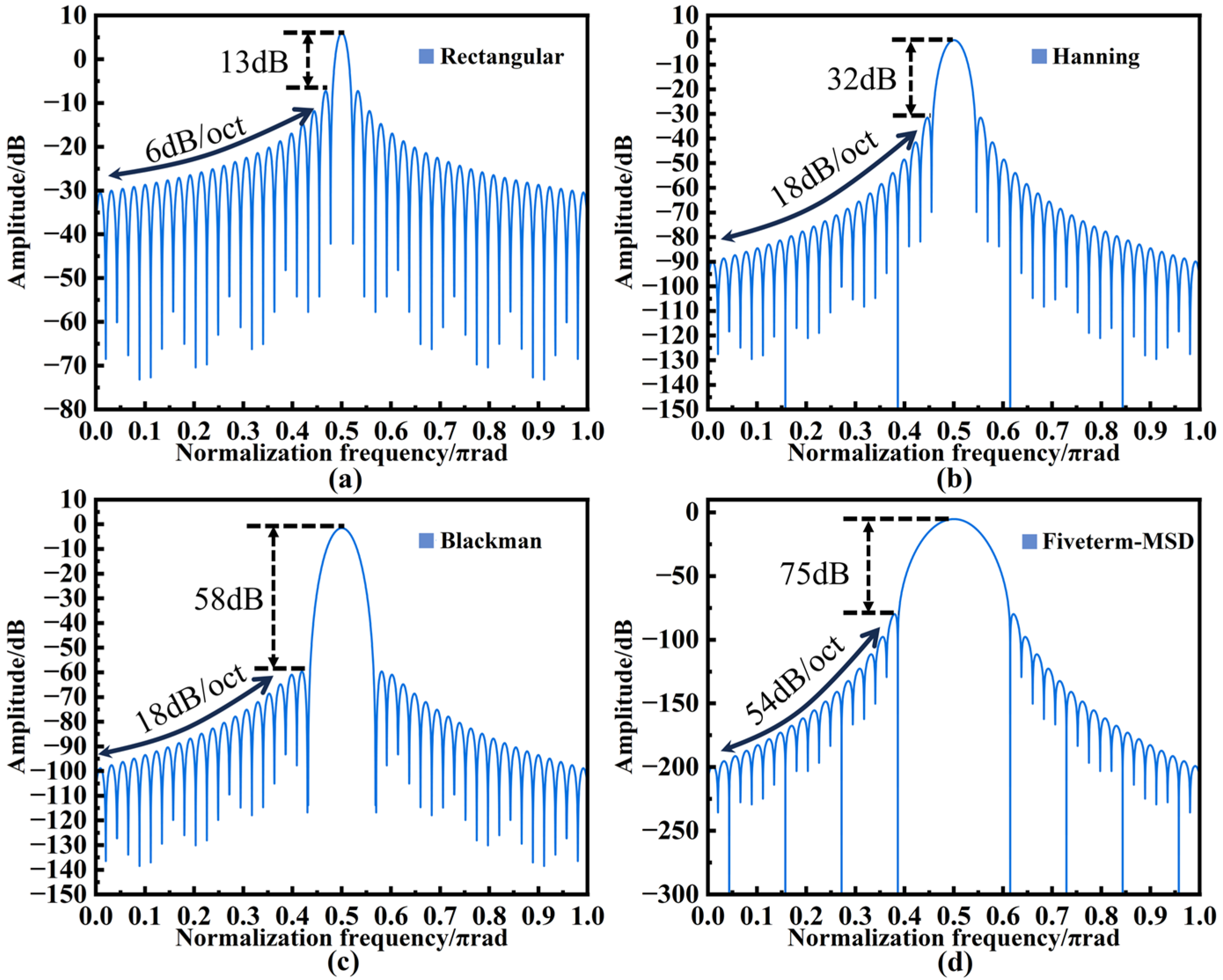
The comparison diagram of classic window functions is shown in Figure 1. Compared to other typical window functions such as RW, Blackman window, and five-term MSD window, the Hanning window, as a representative of traditional cosine combination windows, has a main lobe width of , second only to the RW.
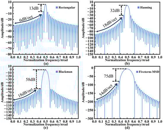
Figure 1.
Comparison of classic window function spectrograms: (a) Rectangular window; (b) Hanning window; (c) Blackman window; (d) Five-term MSD window.
However, the side-lobe attenuation level of the Hanning window is −32 dB, and the attenuation rate is 18 dB/oct. Compared with other window functions, its suppression effect on spectrum leakage is poor, which is not conducive to achieving high-precision wind speed measurement. How to solve the contradiction between the side-lobe attenuation level, side-lobe attenuation rate, and window function main-lobe width is a key research direction to improve the accuracy of the CDWL.
To address this issue, this article utilizes window function self-convolution to enhance the spectral leakage suppression capability of the Hanning window. The window function self-convolution can be defined as [21]:
In Equation (8), denotes the self-convolution order, and is a window function of length . According to the convolution theorem, it can be seen that the convolution of p identical window functions can be obtained as a sequence of the length , and the p order self-convolutional window function of the length can be obtained by padding the zero. The Hanning window frequency domain expression is:
In Equation (9), denotes the RW spectral function, and is the number of cosine terms of the window function. The corresponding p order self-convolutional window function frequency domain expression is:
The p order Hanning window satisfies at the zeros of the spectral lines in the spectrogram of the self-convolutional window, at this point [22]:
Equation (11) holds when , and when , . This leads to a p-order Hanning window self-convolutional window function with a principal flap width of:
When , the spectrogram of the HSCW first- to third-order convolutional window function is shown in Figure 2.
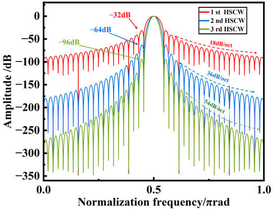
Figure 2.
Comparison of HSCWs of different orders.
3. Simulation
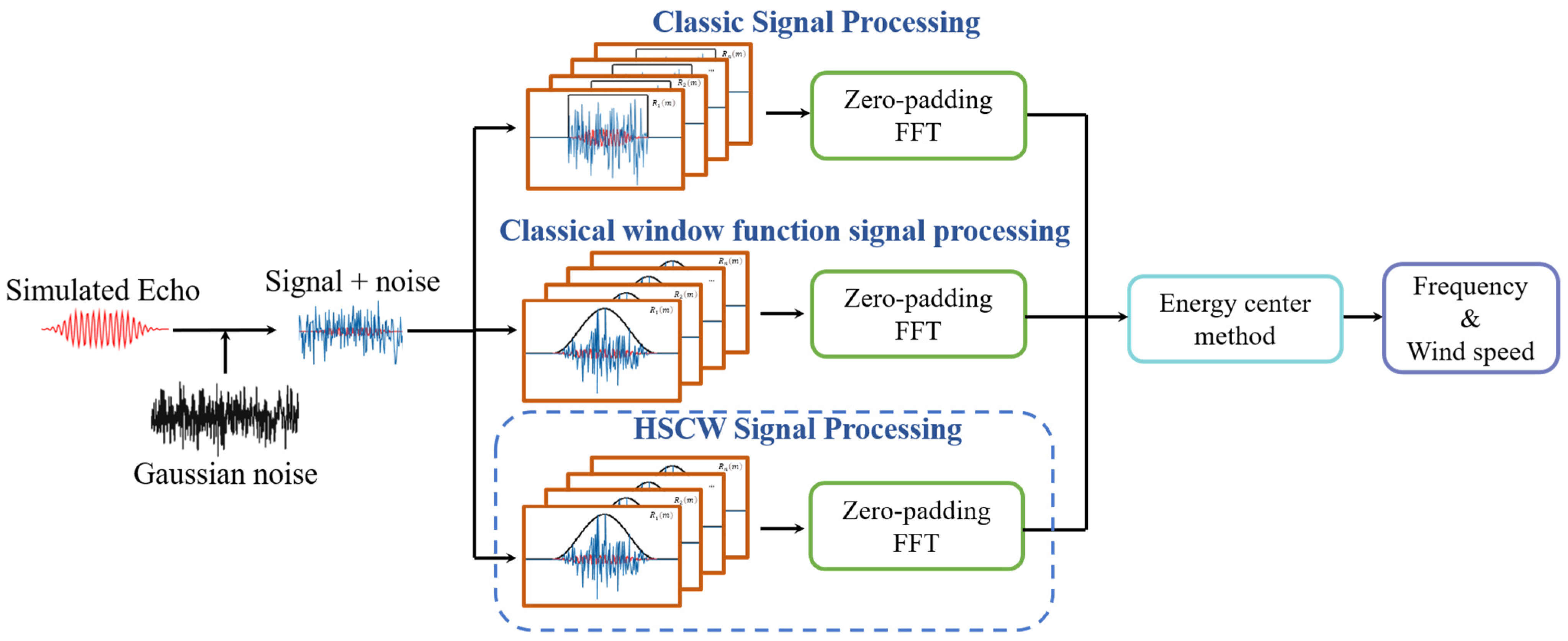
The simulation experiment procedure is shown in Figure 3. A sinusoidal signal (amplitude 1, frequency is , to avoid negative frequencies, signal doppler frequency shift , phase randomly varying in (−π, π)) is generated to simulate Doppler shift and the incoherent accumulation in real systems. A 200 ns wide, 20 kHz repetition frequency pulsed signal, with Gaussian distributed trailing on both sides, is modulated to mimic the atmospheric wind field’s backward Mie scattered echo. After adding Gaussian white noise with a set standard deviation to the simulated echo, RW, classic windows (Blackman and five-term MSD), and different-order HSCW are added in the time domain. The zero-padding FFT algorithm obtains the spectrum, which is then incoherently summed over different periods. Finally, the energy center method is used as a spectral correction algorithm to estimate the frequency of the simulated echo.
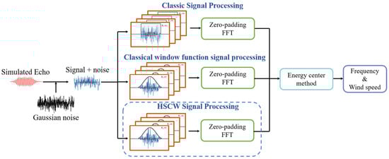
Figure 3.
Simulation experiment flowchart.
At a sampling frequency of 250 MHz, the simulation system mimics the echo signal pulse width with about 50 effective sampling points. To narrow the window function’s main lobe while ensuring the coherent Doppler wind lidar’s spatial resolution, the system takes every 64 points as a range gate. This is equivalent to using the rectangular window function to truncate time domain signals every 64 points.
After zero padding the analog echo signals intercepted by the window function to 128 and 256 points, the results of the FFT algorithm are shown in Figure 4a,b, in which the horizontal coordinates represent the frequency points, the frequency value represented by each unit frequency point is ( is the system sampling rate, and is the number of FFT points), and the vertical coordinates represent the signal amplitude. The black line represents the RW intercepted signal spectrum, and the red line represents the first-order HSCW intercepted signal spectrum. It can be seen that there is a serious spectral leakage of the RW intercepted signal spectrum. The spectral lines of the HSCW intercepted signal are concentrated in the main lobe when compared with the RW interception. However, due to the loss of energy during the interception, the amplitude of the spectral lines is lower. This phenomenon does not lead to the reduction in the system SNR in the case of the system where the signal is superimposed on the noise. A comparison between Figure 4a,b shows that, in the case where the HSCW intercepts a 64-point signal echo, zero padding the echo data to 128 points and 256 points can improve the spectral resolution without affecting the width of the main lobe of the window function. This results in an increase in the number of spectral lines within the main lobe, which hinders the subsequent spectral correction.
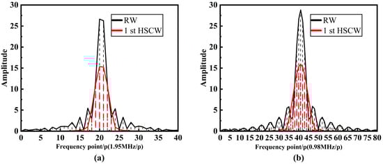
Figure 4.
Comparison of different FFT point sizes: (a) 128-point FFT; (b) 256-point FFT.
To simulate the real-world conditions where wind field echoes are weaker than noise, Gaussian white noise (std = 5) is added to the simulated echo in the range gate. A 128-point FFT is used to obtain the spectrum. As shown in Figure 5a, strong noise prevents the direct extraction of Doppler shift. To improve the SNR, spectral information from different cycles is incoherently accumulated. Figure 5b–f show the results for different accumulation times (N = 250, 500, 1000, 2000, 5000). The horizontal axis represents the frequency points (1.95 MHz each), and the vertical axis is the normalized amplitude. The black, red, blue, brown, purple, and green lines represent the RW, first-order HSCW, second-order HSCW, Blackman, five-term MSD, and third-order HSCW results. For easier analysis, the accumulation results of Gaussian white noise are subtracted after simulating the echoes, and the results of each window function are normalized by dividing by the amplitude of the highest spectral line.
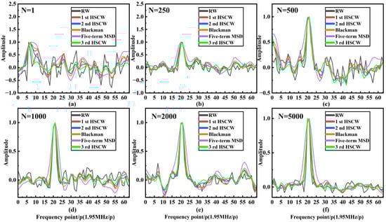
Figure 5.
Comparison of spectral accumulation results under N times of non-coherent accumulation: (a) N = 1; (b) N = 250; (c) N = 500; (d) N = 1000; (e) N = 2000; (f) N = 5000.
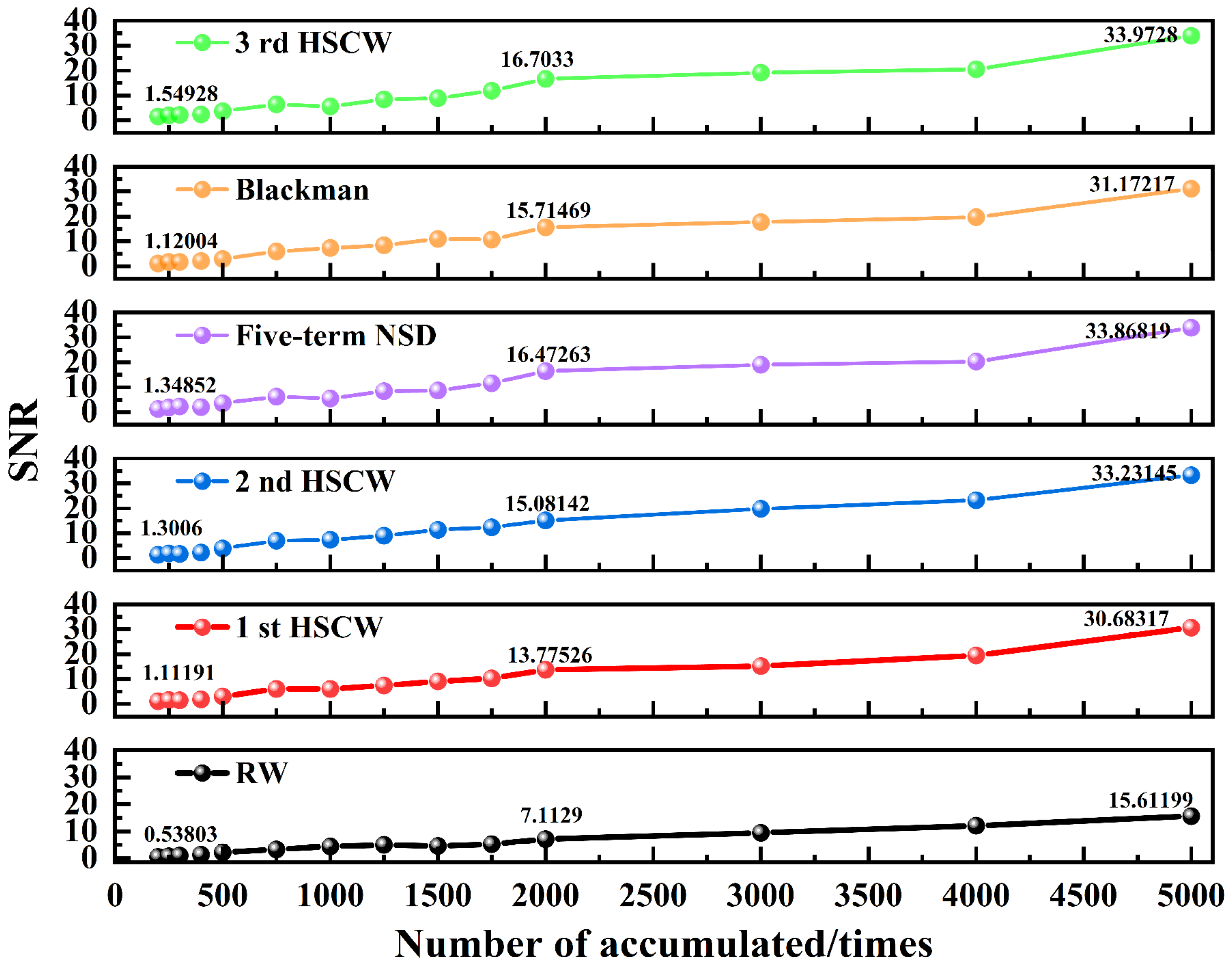
Figure 6 shows the gain process and SNR at different incoherent accumulation times for five window functions. To avoid simulation errors, the experimental results were averaged over 10 time points. Due to the reduced spectral leakage, adding window functions significantly improves the incoherent accumulation compared to the RW. The five-term MSD and second-order HSCW windows offer the highest SNR gain, followed by the Blackman window and first-order HSCW. The second-order HSCW’s incoherent accumulation SNR is 3.28 dB higher than that of the RW.
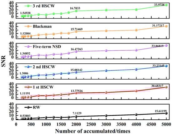
Figure 6.
SNR gain curve.
In order to evaluate the incoherent accumulation results of different window functions, this paper uses the energy center of gravity method to conduct a refined analysis of the frequency spectrum. The number of spectral lines within the main lobe of the window function is represents the number of FFT points, and represents the number of data points). It follows that the RW, Blackman window, and five-term MSD intra-major flap spectral lines are , and .
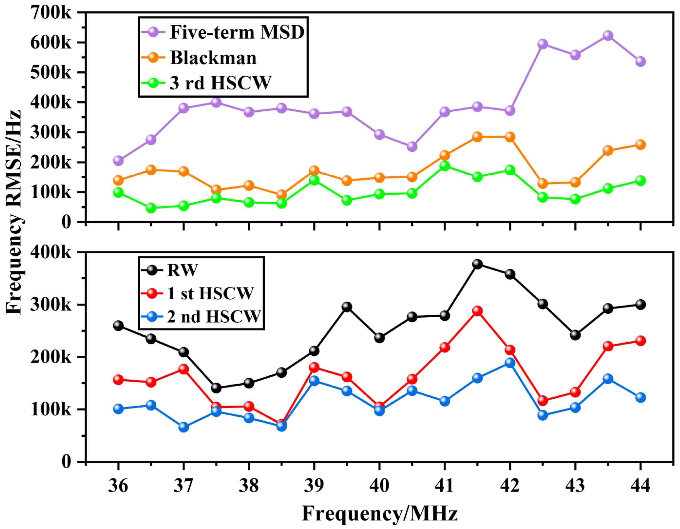
The content shown in Figure 7 shows the spectral RMSE obtained after adding different window functions to the noise containing signals of different frequencies, and after accumulating 5000 times through the spectral incoherence, and then correcting by using the energy center of the gravity algorithm. The horizontal coordinate in the figure represents the frequency of the input signal, and the vertical coordinate represents the computed RMSE.
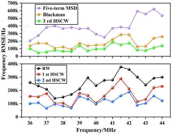
Figure 7.
Comparison of frequency estimation errors.
From the figure, it can be seen that due to the wide width of the main lobe of the five-term MSD window, the energy is released too dispersed in the spectrum, and the results obtained by using the energy center method of correction present a large error. With the increase in the order, the RMSE of the frequencies after processing the data with different orders of HSCW decreases with the increase in the order, and the corresponding average RMSE values of the 1st- to 3rd-order HSCW are 164.2 kHz, 116.7 kHz, and 101.9 kHz, respectively. The average RMSE values obtained by adding the RW and Blackman’s window are 254.9 kHz and 174.3 kHz.
4. Experiment
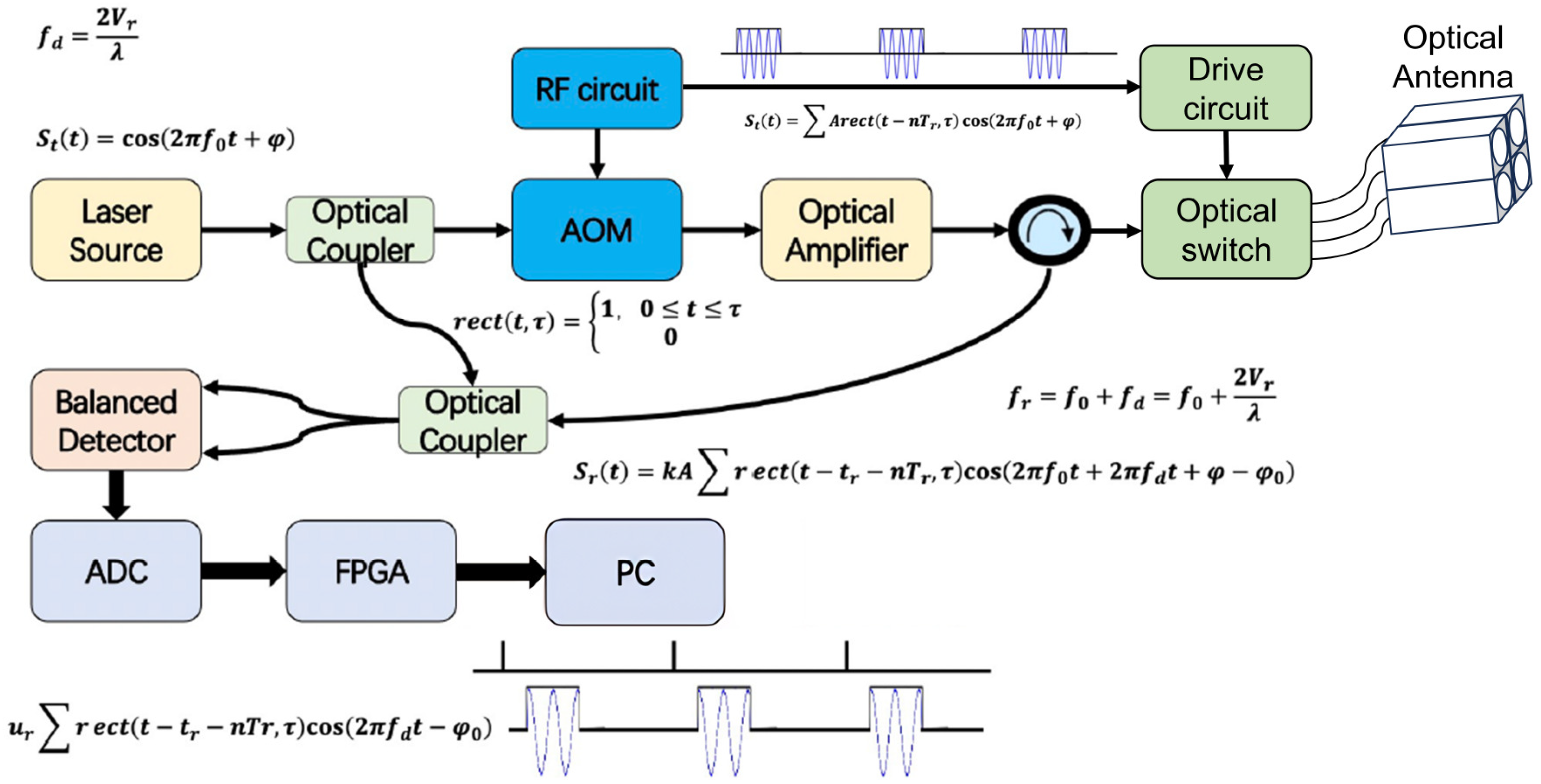
A principal prototype of a pulsed CDWL was designed and constructed on the basis of the aforementioned window function theory study. The system structure is illustrated in Figure 8.
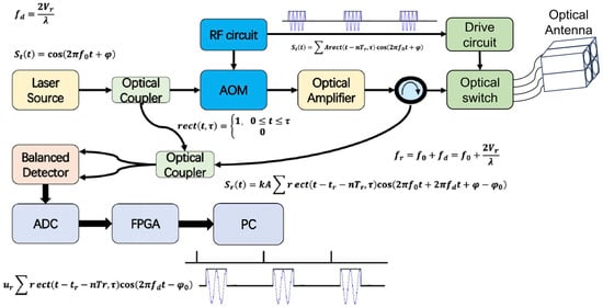
Figure 8.
CDWL system architecture diagram.
The structure of the CDWL can be divided into four main parts: transmitter, receiver, upper computer, and fiber optic connection devices. The transmitter is mainly composed of a laser source, acousto-optic modulator (AOM), erbium-doped fiber amplifier (EDFA), and other devices. The pulsed laser beam emitted by it is transmitted to the target wind field area through a fiber ring resonator and four optical antennas controlled by optical switches. The receiver is mainly composed of a balanced detector, an analog-to-digital converter (ADC), and a Field-Programmable Gate Array (FPGA). The wind field echo signal is coherently mixed with the local oscillator optical signal through a 2 × 2 fiber coupler, and then received by a balanced detector. The wind field echo optical signal is converted into an electrical signal and quantitatively collected through an ADC. The FPGA processes the collected signal by using algorithms to obtain the wind speed and direction results of the target area, which are then displayed on the upper computer. The specific parameters are shown in Table 1.

Table 1.
CDWL prototype parameters.
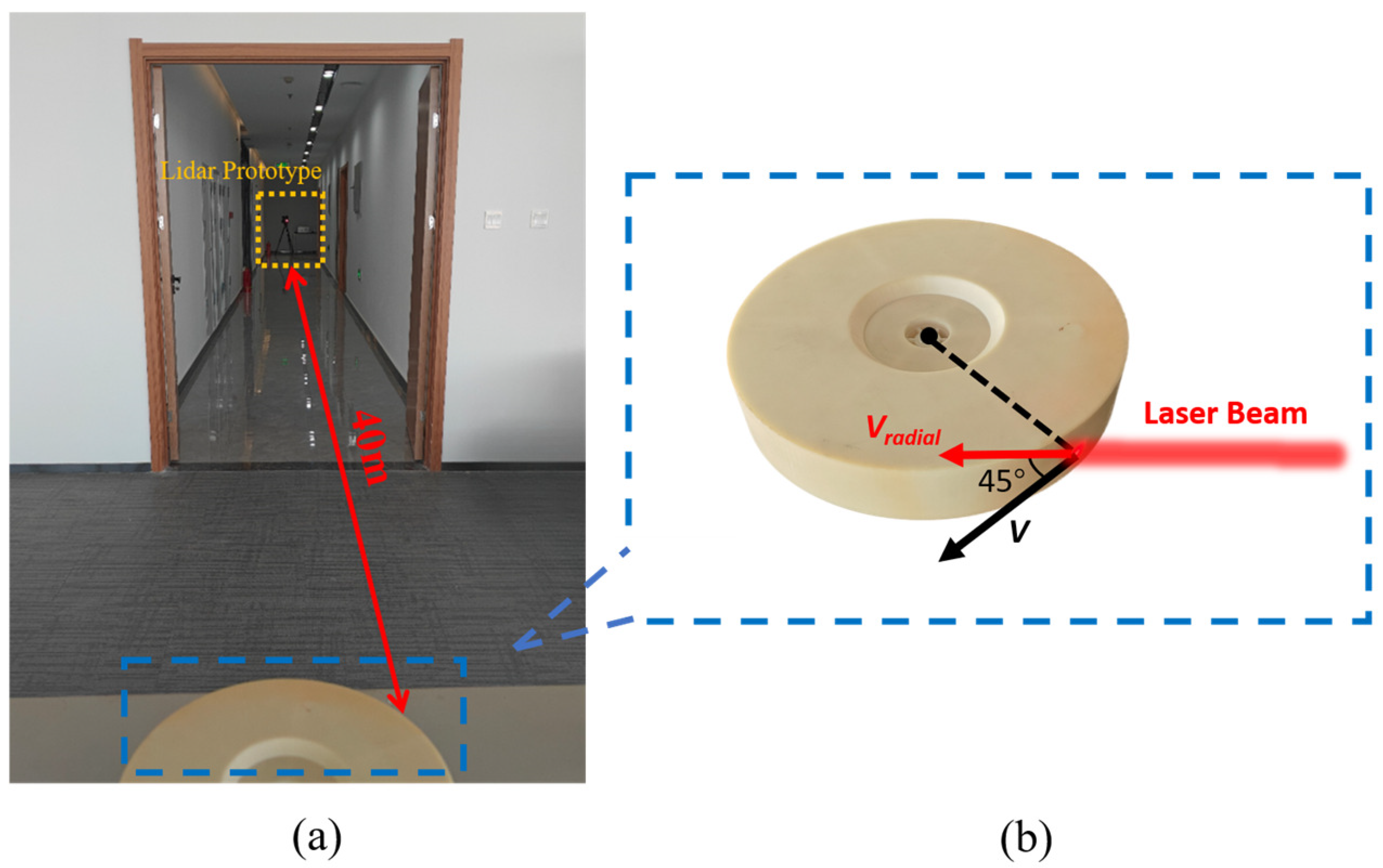
4.1. Turntable Speed Measurement Experiment
The experimental scenario depicted in Figure 9a was devised to ascertain the efficacy of CWDL spectral leakage mitigation through the incorporation of the HSCW. In this experiment, a motor with a turntable is positioned 40 m in front of the CDWL optical system to address the blind zone issue inherent to pulse CDWL, which arises from the reflection off the fiber end face. By adjusting the rotational speed and steering the motor to generate different sizes of Doppler shifts, the test results in the simulation experiments are verified by comparing the frequency inversion results of adding a RW and a HSCW window in the same distance gate. Figure 9b depicts the CDWL laser vertically illuminated on the side of the turntable with a diameter of 30 cm and an incidence angle of 45°.
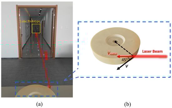
Figure 9.
Turntable experiment scenario: (a) experimental scenario and the distance between the locations of equipment; (b) the irradiation angle of the laser beam.
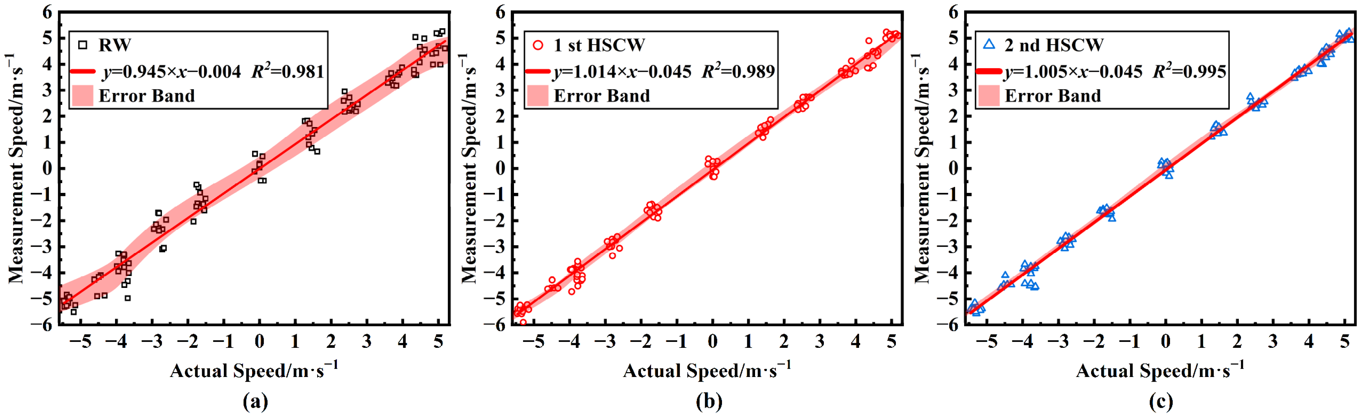
The experiment was conducted using the upper computer to control the rotational speed steering of the turntable. The data underwent 300 instances of incoherent spectrum accumulation following the preprocessing of the RW and HSCW. Subsequently, the velocity inversion results were obtained by employing the energy center of gravity method for spectrum correction. The radial component of the average speed of the turntable during rotation was found to be 4.733 m/s, 4.233 m/s, 3.835 m/s, 2.637 m/s, 1.405 m/s, −0.107 m/s, −1.102 m/s, −1.02 m/s, −2.114 m/s, −3.127 m/s, −4.569 m/s, and −5.124 m/s. The experimental velocity inversion results are shown in Figure 10. In Figure 10, the scatter plot represents the relationship between the actual and measured velocities. The horizontal coordinate of the plot represents the actual turntable radial velocity, the vertical coordinate represents the inverted velocity value after the window function processing, and the red line in the plot represents the result of linear fitting between the actual and measured velocities. The light red area represents the error band of velocity inversion.
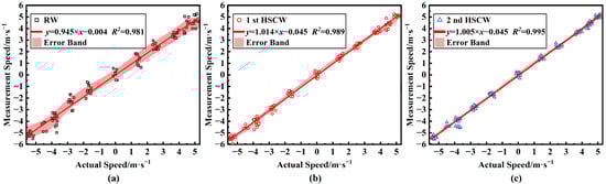
Figure 10.
Comparison of actual and measured speeds for different window functions: (a) rectangular window; (b) 1st HSCW; (c) 2nd HSCW.
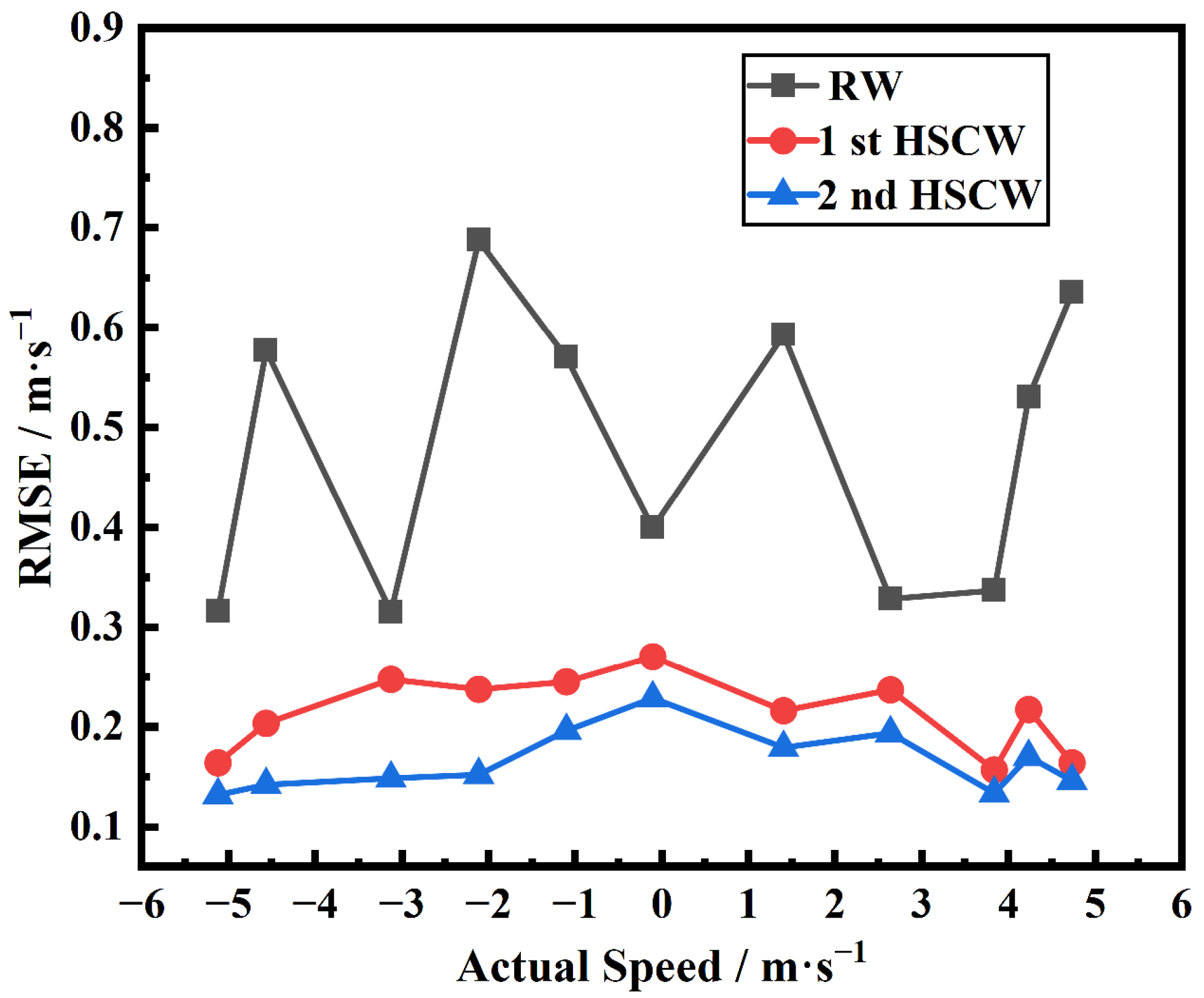
In comparison with the conventional RW function, the incoherent accumulated velocity inversion results obtained through the incorporation of the window function preprocessing demonstrate a closer alignment with the actual velocity outcomes. In order to further analyze the measurement accuracy of the four window functions, the RMSE of the experimental results is compared and analyzed, as shown in Figure 11.
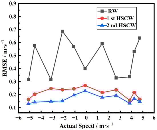
Figure 11.
Comparison of RMSE under different turntable rotation speeds.
This figure shows that the CDWL velocity inversion accuracy is greatly improved after adding the HSCW window function compared with the traditional RW function, and the velocity inversion accuracy of the second-order HSCW window function is even higher compared with the RW and the first-order HSCW. The velocity inversion accuracy under the RW function is 0.481 m/s, and the velocity inversion accuracy after adding the first-order HSCW and the second-order HSCW is 0.214 m/s and 0.173 m/s, respectively.
4.2. Wind Speed Measurement Experiment
On 11 December 2024, the CDWL was placed outdoors at the location coordinates of 43.794713° N, 125.395189° E. Four radial wind speeds were measured by using a four-caliber optical antenna. To verify the accuracy of the measurement results of this CDWL prototype, a commercial CDWL was used as a control in the experiment, and the experimental scenario is shown in Figure 12. The model of the commercial CDWL is the Movelaser Molas NL200, and its specific parameters are shown in Table 2.
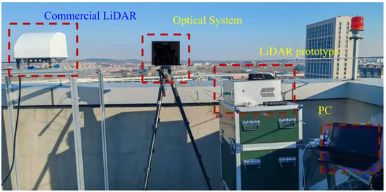
Figure 12.
Outdoor wind farm experimental scene.
Table 2.
Molas NL200 parameters.
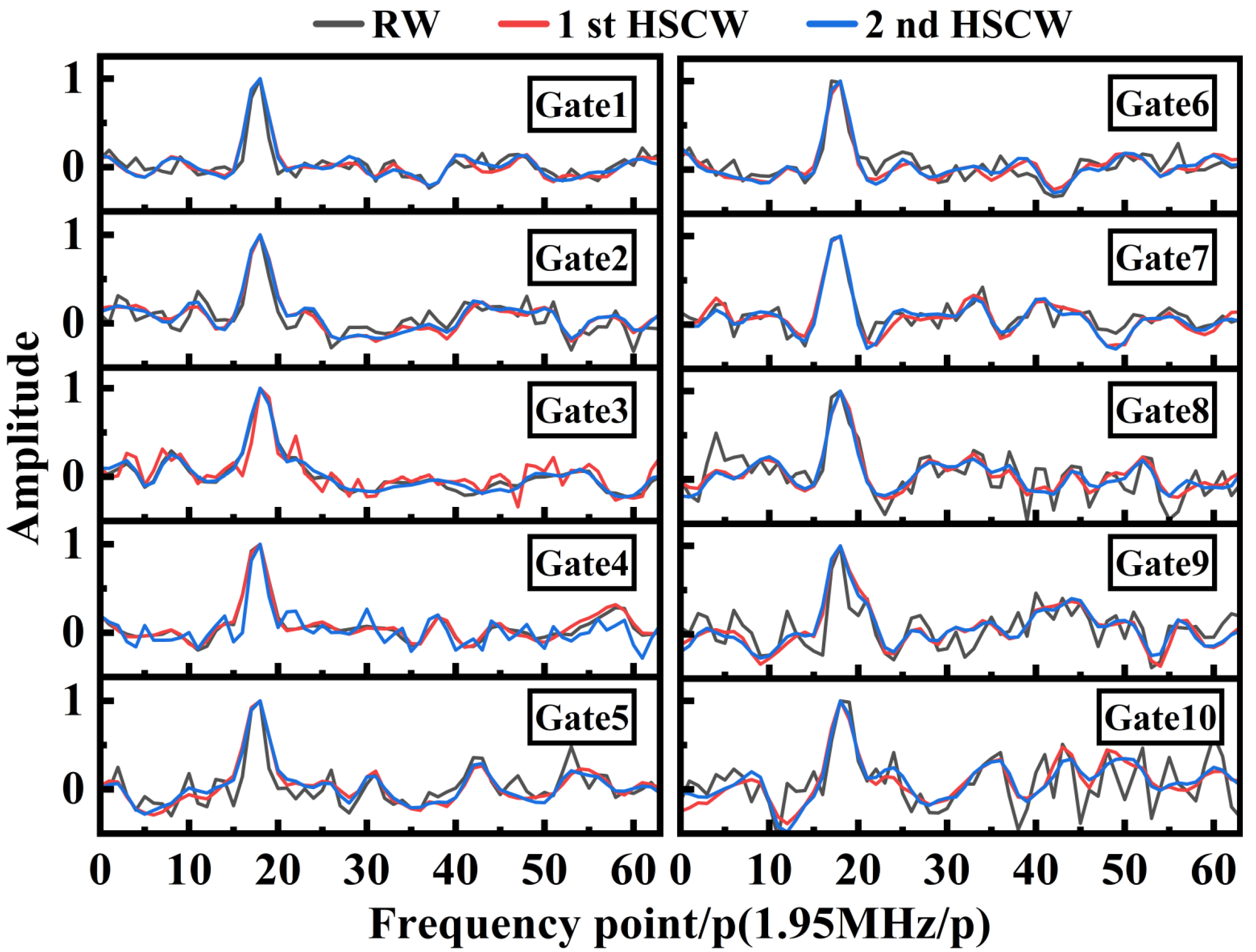
The CDWL sets comprise one distance gate for each of the 64 sampling points, resulting in a total of 10 range gates. The echo signals collected from each distance gate were processed using the traditional RW and HSCW, with the spectral results accumulated 5000 times. The CDWL prototype was designed to divide a total of 10 range gates, each with a width of 38.6 m.
The normalized incoherent accumulation spectra obtained at different range gates are shown in Figure 13. In Figure 13, the horizontal coordinates indicate the frequency points, with each point corresponding to 1.95 MHz. Here, the spectrum result is divided by the amplitude corresponding to the highest spectral line, and the spectrum is normalized for comparison and analysis.
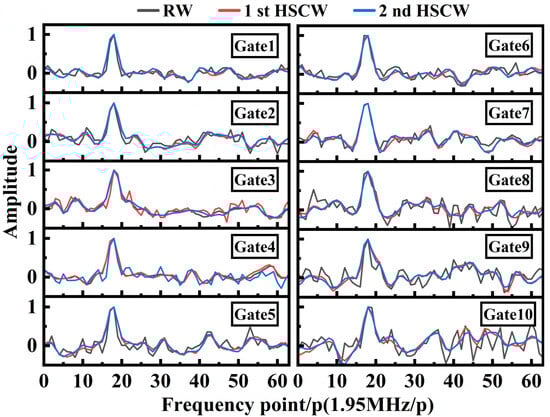
Figure 13.
Normalized spectra of gates at different range gates.
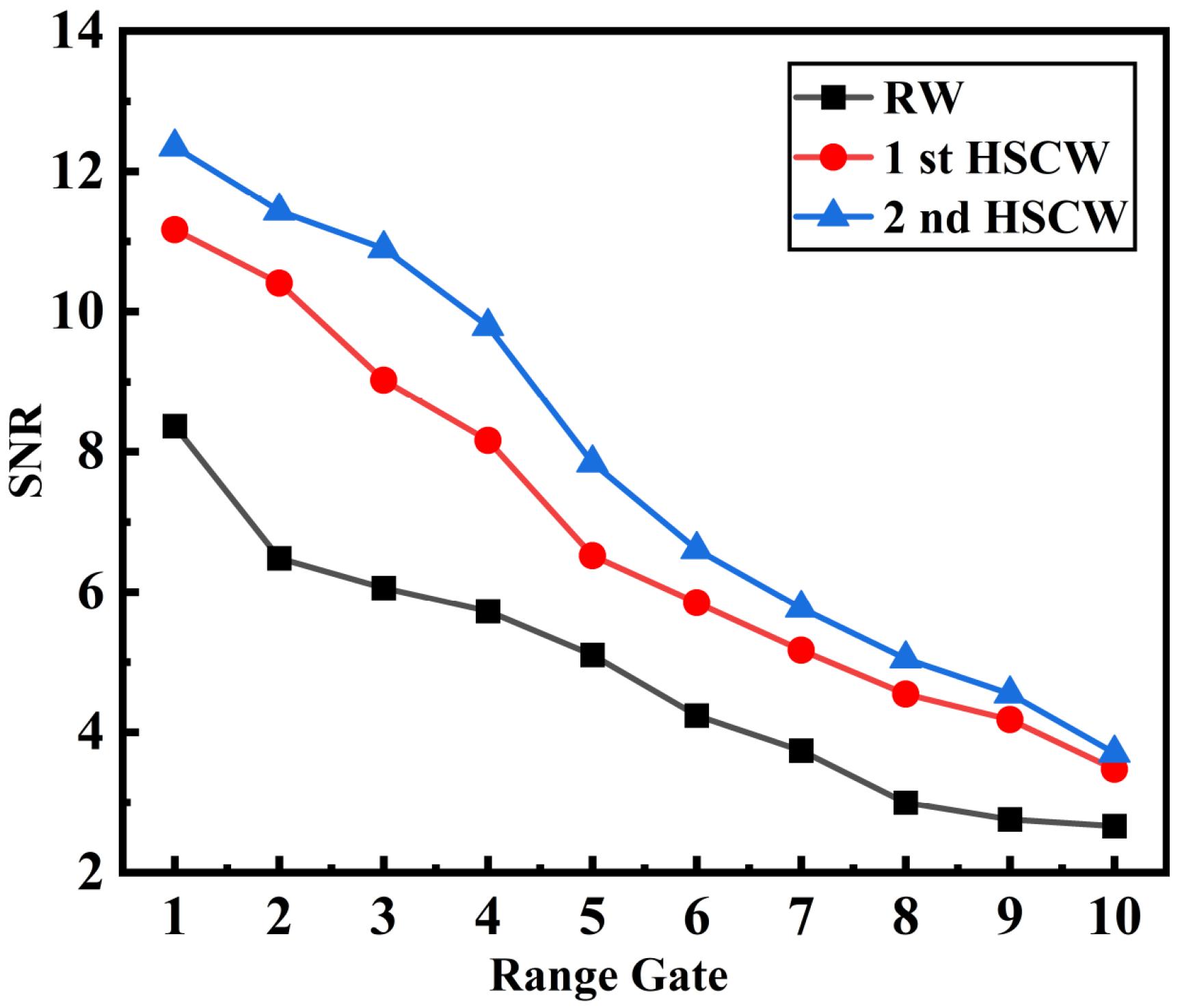
After taking the average of the spectrum accumulation results for 10 different sets of cycles, the variation in the SNR for different range gates is shown in Figure 14, where the horizontal coordinates indicate the individual range gates from near to far, and the vertical coordinates indicate the SNR. Through calculation, the SNR after adding the second-order HSCW and the first-order HSCW has increased by 2.06 dB and 1.52 dB, respectively, compared with that of the RW.
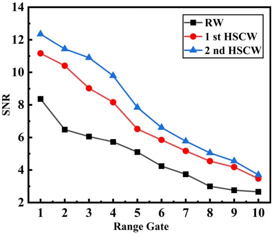
Figure 14.
Range gate SNR change.
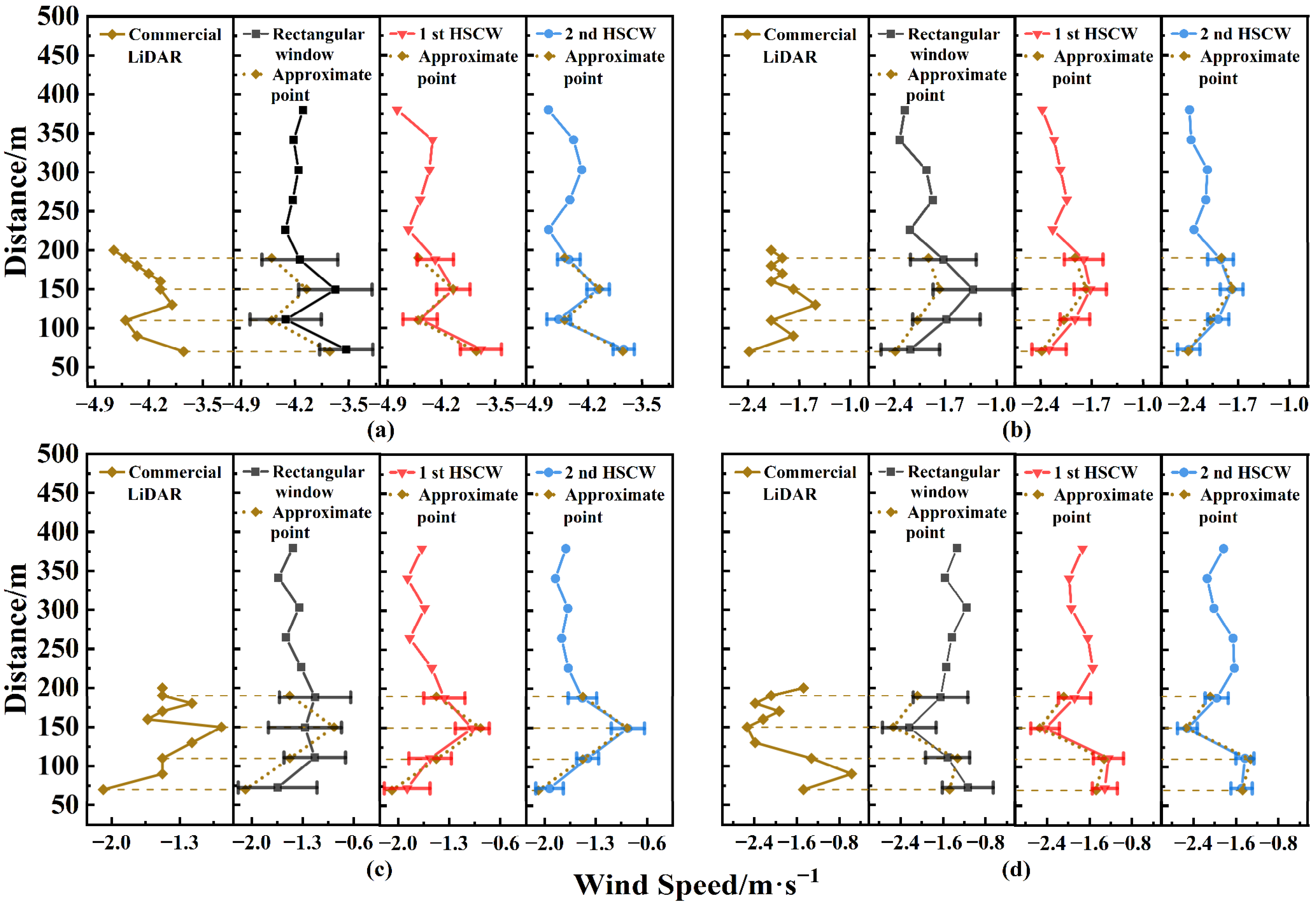
A comparison of the four-caliber wind speed inversion results is presented in Figure 15.
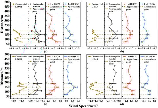
Figure 15.
Retrieval results of wind speed in different line of sight directions: (a) upper left line of sight; (b) upper right line of sight; (c) lower left line of sight; (d) lower right line of sight.
Figure 15a–d illustrate the comparison of radial wind speeds measured by each aperture of the four-caliber CDWL. The black, red, and blue curves represent the wind speed inversion results obtained by adding the RW, the first-order HSCW, and the second-order HSCW, respectively. The brown curves represent the results of the wind speeds measured by the commercial CDWL. Due to the closer detection distance and higher spatial and temporal resolution of the commercial CDWL, only a portion of the points in the experimental system can be approximated (approximate points are located at 70 m, 110 m, 150 m, and 190 m). Then, these approximate points of the CDWL prototype were compared with the commercial CDWL (as shown by the brown dashed line in the figure), and the results showed that the CDWL prototype system with the added HSCW had greater consistency with the wind speed measurement results of the commercial CDWL. In addition, according to the error bars at the approximate points, it can be seen that compared with the first-order HSCW, the difference between the wind speed inversion results of the second-order HSCW at the approximate point position and the commercial CDWL inversion results is relatively small.
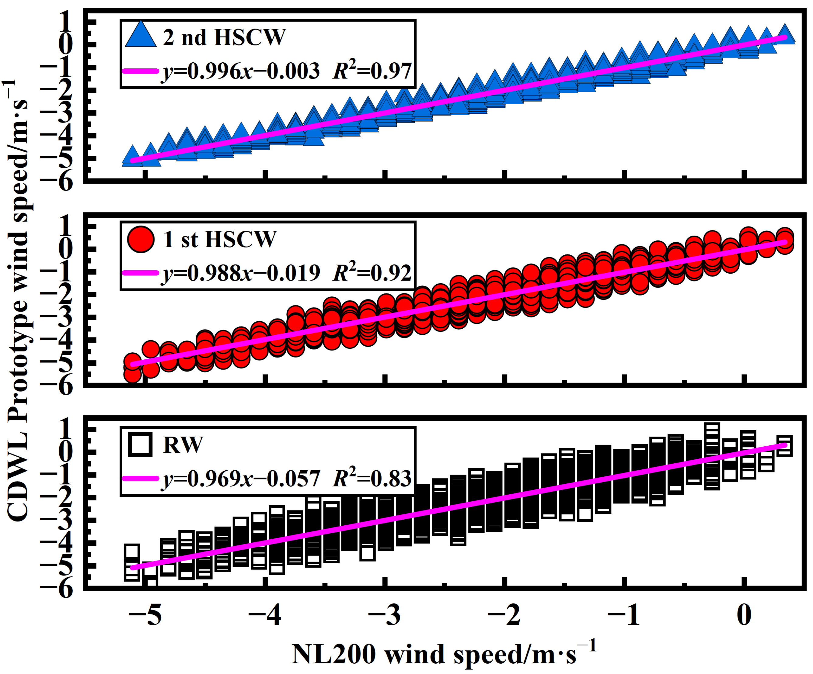
In this paper, 500 sets of wind speed inversion results obtained from the measurements of four independent apertures at a distance of 110 m (a total of 2000 data points) are selected for linear analysis. The results of this analysis are presented in Figure 16. The horizontal coordinates in this figure represent the wind speed inversion results of the commercial CDWL at the 110-meter-point location, while the vertical coordinates represent the wind speed inversion results of the CDWL prototype. As can be clearly discerned from Figure 16, the inversion results processed by utilizing the second-order HSCW are more closely aligned with the commercial CDWL inversion results, exhibiting a higher degree of fit.
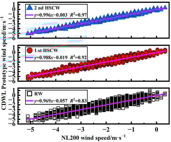
Figure 16.
Linear fitting results of wind speed.
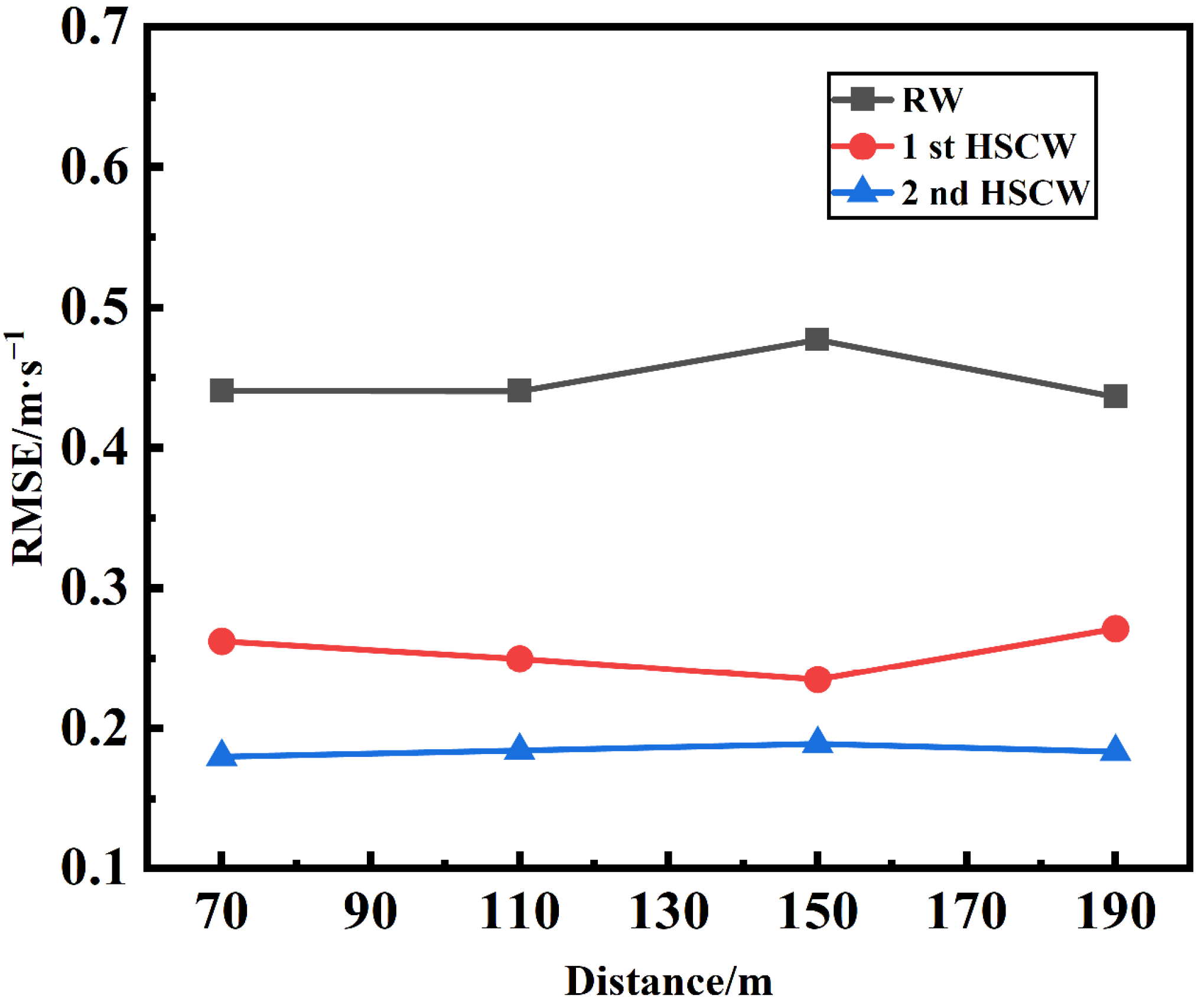
Figure 17 shows the RMSE of wind speed inversion for four approximate points after adding different window functions. At the same distance, after determining the wind speed inversion results of the commercial CDWL as the true values during wind speed measurement, we used 500 sets of experimental data from each of the four line of sight directions for error analysis. In the figure, the horizontal axis represents the distance, and the vertical axis represents the average RMSE of 2000 sets of data. The average RMSE of the four approximate points for calculating the wind speed results of the CDWL prototype using the RW, first-order HSCW, and second-order HSCW inversion are 0.449 m/s, 0.266 m/s, and 0.184 m/s, respectively.
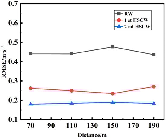
Figure 17.
RMSE of approximate points.
5. Conclusions
This paper proposes using the HSCW to preprocess the pulsed CDWL’s wind speed echo, aiming to solve the traditional inversion algorithm’s spectral leakage problem. The first- and second-order HSCW can boost the system’s incoherent accumulation SNR. The simulation experimental results demonstrate the excellent performance of the HSCW. Compared with the RW, its SNR has increased by 3.28 dB. Meanwhile, the RMSE values of the first- to third-order HSCW are as low as 164.2 kHz, 116.7 kHz, and 101.9 kHz, respectively.
To assess the HSCW’s effectiveness in wind speed inversion, four caliber inversion results were compared with a commercial pulsed CDWL. Linear fitting results at nearby points show that the second-order HSCW’s measurements are closer to the commercial one than the RW and first-order HSCW. The RMSE of the second-order HSCW is 0.184 m/s, while the RW is 0.449 m/s, and the first-order HSCW is 0.266 m/s.
It cannot be denied that compared to traditional window functions, the HSCW algorithm has a higher delay due to its self-convolution characteristics. As the order increases, the algorithm delay also increases, but it is still significantly better than the adaptive distance gate algorithm delay. In the future, the HSCW order can be adaptively selected to further enhance the real-time performance in complex environments.
Author Contributions
Conceptualization, S.T.; Investigation, Z.H.; Writing—original draft, C.S.; Writing—review & editing, P.L. and X.Y.; Supervision, N.L. All authors have read and agreed to the published version of the manuscript.
Funding
This research was funded by Changchun University of Science and Technology, grant number [2022YFB2903402].
Institutional Review Board Statement
Not applicable.
Informed Consent Statement
Not applicable.
Data Availability Statement
The original contributions presented in the study are included in the article, further inquiries can be directed to the corresponding author.
Conflicts of Interest
The authors declare no conflicts of interest.
References
- Frehlich, R.; Cornman, L. Coherent Doppler Lidar Signal Spectrum with Wind Turbulence. Appl. Opt. 1999, 38, 7456. [Google Scholar] [CrossRef]
- Wang, K.; Gao, C.; Lin, Z.; Wang, Q.; Gao, M.; Huang, S.; Chen, C. 1645 Nm Coherent Doppler Wind Lidar with a Single-Frequency Er:YAG Laser. Opt. Express 2020, 28, 14694. [Google Scholar] [CrossRef]
- Song, Y.; Han, Y.; Su, Z.; Chen, C.; Sun, D.; Chen, T.; Xue, X. Denoising Coherent Doppler Lidar Data Based on a U-Net Convolutional Neural Network. Appl. Opt. 2024, 63, 275. [Google Scholar] [CrossRef] [PubMed]
- Yuan, J.; Xia, H.; Wei, T.; Wang, L.; Yue, B.; Wu, Y. Identifying Cloud, Precipitation, Windshear, and Turbulence by Deep Analysis of the Power Spectrum of Coherent Doppler Wind Lidar. Opt. Express 2020, 28, 37406–37418. [Google Scholar] [CrossRef]
- Kliebisch, O.; Uittenbosch, H.; Thurn, J.; Mahnke, P. Coherent Doppler Wind Lidar with Real-Time Wind Processing and Low Signal-to-Noise Ratio Reconstruction Based on a Convolutional Neural Network. Opt. Express 2022, 30, 5540. [Google Scholar] [CrossRef] [PubMed]
- Lin, R.; Guo, P.; Chen, H.; Chen, S.; Zhang, Y. Smoothed Accumulated Spectra Based wDSWF Method for Real-Time Wind Vector Estimation of Pulsed Coherent Doppler Lidar. Opt. Express 2022, 30, 180. [Google Scholar] [CrossRef] [PubMed]
- Hu, Y.; Xie, C.; Zhou, H.; Xing, K.; Wang, B.; Wang, Y. Research on Optimizing the Optical Local-Oscillator Power of Coherent Doppler LiDAR to Enhance Wind Velocity Measurements. J. Instrum. 2024, 19, P10028. [Google Scholar] [CrossRef]
- Abdelazim, S.; Santoro, D.; Arend, M.F.; Moshary, F.; Ahmed, S. Development and Operational Analysis of an All-Fiber Coherent Doppler Lidar System for Wind Sensing and Aerosol Profiling. IEEE Trans. Geosci. Remote Sens. 2015, 53, 6495–6506. [Google Scholar] [CrossRef]
- Xu, G.; Yin, W.; Li, C.; Chen, Y.; Feng, L.; Zhou, D. Research on high resolution range-gate adaptive technology of coherent wind lidar. Infrared Laser Eng. 2021, 50, 20210187. [Google Scholar] [CrossRef]
- Zhu, X.; Liu, J.; Bi, D.; Zhou, J.; Diao, W.; Chen, W. Development of All-Solid Coherent Doppler Wind Lidar. Chin. Opt. Lett. 2012, 10, 012801–012803. [Google Scholar] [CrossRef]
- Zhang, D.; Zhao, H.; Yang, J. A High Precision Signal Processing Method for Laser Doppler Velocimeter. Optik 2019, 186, 155–164. [Google Scholar] [CrossRef]
- Yang, Q.; Qu, X. High-Precision Harmonic Analysis Algorithm Based on Five-Term MSD Second-Order Self-Convolution Window Four-Spectrum-Line Interpolation. Mob. Netw. Appl. 2023, 28, 579–585. [Google Scholar] [CrossRef]
- Kim, K.-W.; Park, J.-J.; Kim, M.-D.; Lee, J. Spectral Leakage Reduction of Power-Delay-Doppler Profile for Mm-Wave V2I Channel. In Proceedings of the 2018 International Conference on Information and Communication Technology Convergence (ICTC), Jeju, Republic of Korea, 17–19 October 2018; IEEE: New York, NY, USA, 2008; pp. 346–350. [Google Scholar]
- Wen, H.; Zhang, J.; Meng, Z.; Guo, S.; Li, F.; Yang, Y. Harmonic Estimation Using Symmetrical Interpolation FFT Based on Triangular Self-Convolution Window. IEEE Trans. Ind. Inform. 2015, 11, 16–26. [Google Scholar] [CrossRef]
- Xu, F.; Zhao, Y.; Ni, L.; Wu, Q.; Xia, H. Two-Dimensional Hanning Self-Convolution Window for Enhancing Moiré Fringe Alignment in Lithography. Mech. Syst. Signal Process. 2024, 208, 111052. [Google Scholar] [CrossRef]
- Xu, X.; Luo, M.; Tan, Z.; Pei, R. Echo Signal Extraction Method of Laser Radar Based on Improved Singular Value Decomposition and Wavelet Threshold Denoising. Infrared Phys. Technol. 2018, 92, 327–335. [Google Scholar] [CrossRef]
- Liang, N.; Yu, X.; Lin, P.; Chang, S.; Zhang, H.; Su, C.; Luo, F.; Tong, S. Pulse Accumulation Approach Based on Signal Phase Estimation for Doppler Wind Lidar. Sensors 2024, 24, 2062. [Google Scholar] [CrossRef]
- Gabor, D. Theory of Communication. Part 3: Frequency Compression and Expansion. J. Inst. Electr. Eng. Part III Radio Commun. Eng. 1946, 93, 445–457. [Google Scholar] [CrossRef]
- Kameyama, S.; Ando, T.; Asaka, K.; Hirano, Y.; Wadaka, S. Compact All-Fiber Pulsed Coherent Doppler Lidar System for Wind Sensing. Appl. Opt. 2007, 46, 1953. [Google Scholar] [CrossRef]
- Wang, C.; Xia, H.; Liu, Y.; Lin, S.; Dou, X. Spatial Resolution Enhancement of Coherent Doppler Wind Lidar Using Joint Time–Frequency Analysis. Opt. Commun. 2018, 424, 48–53. [Google Scholar] [CrossRef]
- Ji, Y.; Yan, W.; Wang, W. Supraharmonic Detection Algorithm Based on Interpolation of Self-Convolutional Window All-Phase Compressive Sampling Matching Pursuit. Information 2024, 15, 127. [Google Scholar] [CrossRef]
- Xu, Y.; Du, Y.; Li, Z.; Xi, L.; Liu, Y. Harmonic Parameter Online Estimation in Power System Based on Hann Self-Convolving Window and Equidistant Two-Point Interpolated DFT. MAPAN 2020, 35, 69–79. [Google Scholar] [CrossRef]


Disclaimer/Publisher’s Note: The statements, opinions and data contained in all publications are solely those of the individual author(s) and contributor(s) and not of MDPI and/or the editor(s). MDPI and/or the editor(s) disclaim responsibility for any injury to people or property resulting from any ideas, methods, instructions or products referred to in the content. |
© 2025 by the authors. Licensee MDPI, Basel, Switzerland. This article is an open access article distributed under the terms and conditions of the Creative Commons Attribution (CC BY) license (https://creativecommons.org/licenses/by/4.0/).