Abstract
The stitching of bone stick fragments is of great significance for the inheritance of and research into the outstanding traditional culture of the Western Han Dynasty. Focused on the problem that the existing methods have a low bone stick fragment stitching success rate due to their complex edges, this paper proposes a bone stick fragment stitching method based on improved corner detection, which strengthens the features of broken edges and improves the success rate of stitching. First, the maximum outer contour of the bone stick fragment is obtained using connectivity analysis. Then, the broken edge features are enhanced by combining multi-scale and multi-stage corner detection, as well as a double screening mechanism of local template and corner density analysis. On this basis, the maximum outer contour is segmented using a region segmentation method based on corner features. Then, a priority matching strategy is used to perform multi-dimensional sequential priority matching of corner features for the densest segments and to match other contour segments in the order of density. Finally, based on the matching results, the bone stick fragment is stitched exactly and restored. Experimental results show that compared with other algorithms, the average proportion of broken corners when using the method in this paper is increased by about 44.89%, and the average comprehensive weighted similarity is increased by about 32.42%, which meets the needs of bone stick fragment stitching.
1. Introduction
Nearly 30,000 bone sticks were unearthed from the ruins of the Han Dynasty’s Chang’an City in Weiyang Palace. These bone sticks are inscribed with a large number of texts and have a clear archival nature. They cover almost the entire official hierarchy system, the offering of goods, and the development status of various industries during the Western Han Dynasty, and are of great significance for the inheritance of and research into the outstanding traditional culture of the Western Han Dynasty. Due to the long period of time that has passed, most of the bone sticks have become fragments due to wear and tear, which has greatly affected the research progress. Therefore, it is necessary to stitch the broken bone stick [1,2,3]. At present, the stitching of traditional bone stick fragments is performed manually, which has the problems of low stitching efficiency and high restoration costs. With the development of computer vision and image processing technology, using a computer to stitch and restore bone stick fragments can not only greatly improve stitching efficiency and reduce stitching costs, but can also avoid the secondary damage that may be caused to bone stick fragments during the manual stitching process [4].
Bone stick fragments, like bronze fragments, are mostly small, thin, irregular fragments. The surface is corroded and damaged, making it difficult to extract color and texture features. Therefore, it is more appropriate to choose a contour-based method for 2D fragment stitching [5,6]. There are many common contour-based 2D fragment stitching methods. For example, Lin et al. [7] and others proposed a fragment stitching method based on shape matching, which uses contour features for fragment matching and can obtain more accurate matching results. However, this method can only handle local fragment stitching tasks and is not effective for fragments with irregular shapes and complex contour features. Yu et al. [8] and others proposed a curve-matching method based on the Freeman chain code description. This method uses Freeman chain code to describe the curve outline, which can effectively avoid the noise and rotation problems that may be encountered with traditional coordinate description methods. It is suitable for processing large amounts of data, but for complex outlines, it is not only computationally intensive but may also produce large matching errors. Shi [9] and others used Freeman chain codes for contour representation and the edge and corner features for feature matching, but their matching method is too simple and prone to mismatches. Lin et al. [10] and others proposed a method for virtually stitching small fragments of bronzeware using curvature features. This method uses the local maximum curvature to extract the corner points on the edges of the small bronze fragments, removes pseudo-corner points and useless corner points, and then uses the obtained corner sequence for matching, which achieves relatively good stitching results. However, the accuracy of removing useless corner points during the corner point calculation process is low, and the matching method of the longest common subsequence is also too strict.
Although matching directly using the maximum outer contour of the bone stick fragment is an intuitive stitching method, it may result in a high matching error due to the large amount of calculation required and the difficulty of matching the original matching fracture surfaces one by one due to the wear on the edges of the bone stick fragment. Therefore, it is necessary to extract features from the maximum outer contour of the bone stick fragment and select corner points with rotational and translational invariance as local feature points of the contour curve. However, traditional and existing improved corner detection methods [10,11,12,13,14,15] are mostly aimed at simple-shaped samples or specific cultural relic fragments. Although methods such as multi-scale detection or pseudo-corner point screening can improve detection speed and accuracy in some scenarios, they often have difficulty extracting enough valid corner points when faced with complex fracture edges and dense feature areas of bone stick fragments, and even generate large numbers of pseudo-corner points. In addition, when dealing with bone stick fragments with complex edge features and irregular shapes, existing stitching algorithms are prone to stitching offset and overlap problems. In particular, the dense feature areas along the fracture edges are not fully utilized during the corner feature extraction and matching process, resulting in a low stitching success rate and making it difficult to meet the basic needs of cultural relic restoration.
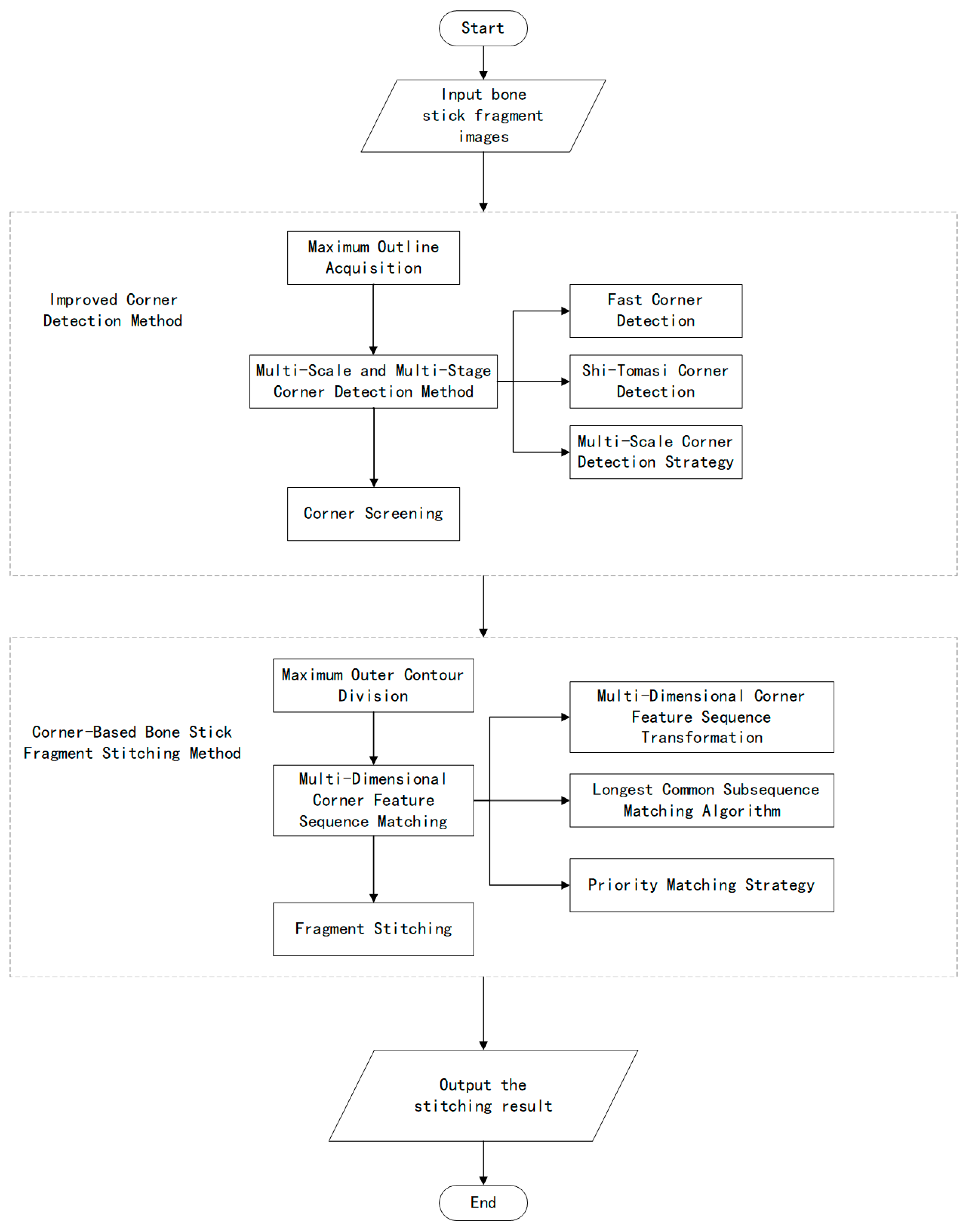
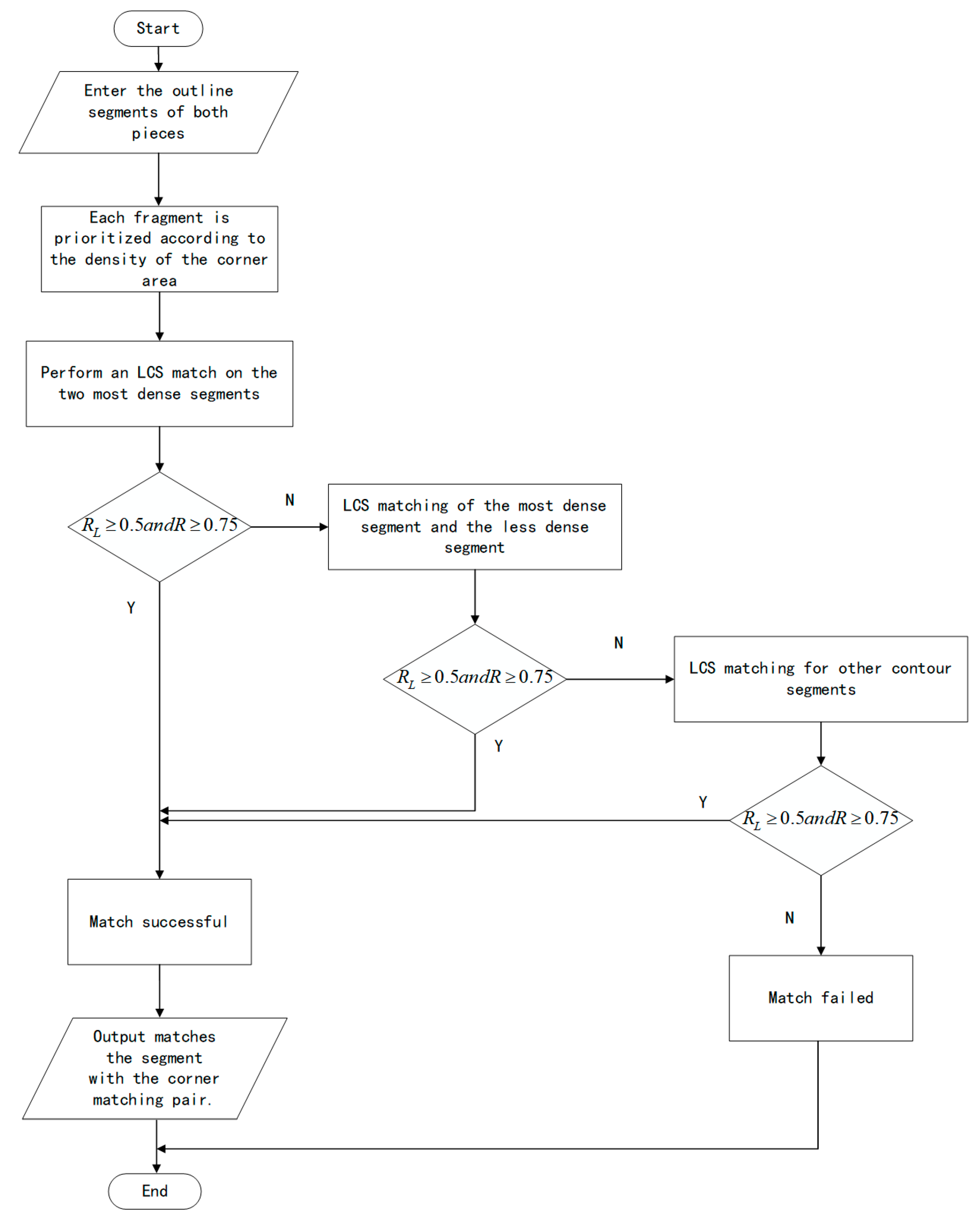
In response to the above problems, this paper proposes a bone stick fragment stitching method based on improved corner detection. Figure 1 shows the specific process of this method. First, the maximum outer contour of the bone stick fragment is obtained. Then, by combining multi-scale and multi-stage corner detection, as well as using the double corner screening mechanism of local template and corner density analysis, the characteristics of the broken edges are enhanced to obtain the set of corners on the maximum outer contour. On this basis, the maximum outer contour of the bone stick fragment is segmented into four parts using a region segmentation method based on the corner distribution characteristics. The contour segments are prioritized for matching according to the degree of overlap with the corners in the areas with the highest and second highest concentrations of fracture edges. The higher the degree of overlap, the higher the corner density and the greater the likelihood that it is a fracture edge. At this time, the contour segment with the highest corner density is the densest segment. Then, the prioritized matching strategy is used to perform a sequence of prioritized matching of the most densely packed segments based on their corner features, and the other segments are matched in order of density. Finally, based on the matching results, the bone stick fragments are accurately stitched and restored.
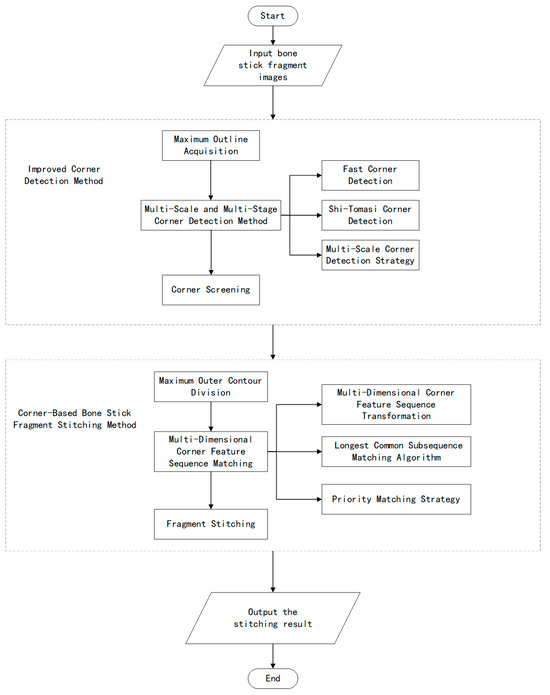
Figure 1.
Method flowchart.
2. Improved Corner Detection Method
In this paper, an improved corner detection method based on fracture edge features is proposed to achieve the preferential extraction of significant corner points at fracture edges, and at the same time to reduce invalid corner points at non-fracture edges to strengthen the fracture edge features, which specifically includes maximum outer contour acquisition, multi-scale and multi-stage corner detection methods, and corner screening.
2.1. Maximum Outline Acquisition
The texture, color, and material characteristics of the bone stick surface contain a lot of redundant information. If feature extraction is performed directly on the image of the bone stick fragment, the rust and cracks on the surface and the surrounding noise will generate a large number of features that are not on the fracture surface. Filtering these features that are not on the maximum outer contour will result in excessive computing. Therefore, by obtaining the maximum outer contour, other unnecessary redundant information can be removed, and only the complete and representative maximum outer contour is retained to ensure the accuracy of subsequent corner detection based on the maximum outer contour and the effectiveness of stitching. In this paper, a maximum outer contour extraction method based on the Suzuki–Abe algorithm is used [16]. This method, based on Canny edge detection [17], finds all connected contours by connectivity analysis and selects the contour with the largest area as the maximum outer contour by the area calculation method to obtain all of its coordinate point sets.
2.2. Multi-Scale and Multi-Stage Corner Detection Method
2.2.1. FAST Corner Detection
First, the FAST corner detection algorithm is used to perform a preliminary corner detection on the maximum outer contour of the acquired bone stick fragment. The FAST corner detection algorithm can quickly screen a large number of potential corners, reduce computational complexity, and maintain a high detection speed, which is very suitable for processing a large number of bone stick fragment contour point coordinates [18]. Due to the complex edge features of the bone stick fragment, the goal of the preliminary detection stage is to capture as many possible corners as possible, especially those that are located at the break edge and in its adjacent area.
The FAST corner detection algorithm mainly determines whether a pixel is a corner by quickly determining the gray level in its neighborhood. The main algorithm steps are as follows:
- (1)
- Neighboring pixel selection. For each contour point , a circular area with a radius of 3 centered at this point is selected, containing 16 pixels which are numbered , , … . This selection method helps to quickly determine whether the gray level changes around this point are sufficient to make it a corner.
- (2)
- Gray-scale comparison. The gray value of the central pixel is set to be , and a threshold is defined. Then, for each neighboring pixel , if or is satisfied, it is considered that may be a corner.
- (3)
- Continuity determination. Whether or not there are more than consecutive pixels in the neighborhood that meet the above gray difference conditions is checked. If so, point is marked as a corner. This strategy can quickly screen out significant corners from a large number of points, reducing computational complexity.
- (4)
- Non-maximum suppression. Non-maximum suppression is performed on the detected corners to eliminate redundant corners, retain the corners with the strongest response in a local region, and obtain the initial corner set .
Among these, the selection of parameters has a significant impact on the detection results. The threshold parameter controls the sensitivity to gray-scale changes, and its setting is directly related to the effect of preliminary corner screening. It is usually adjusted based on experimental sample data to ensure that a sufficient number of potential corners can be detected in complex edge areas, especially broken edges. The minimum neighborhood connectivity parameter affects the corner determination conditions. A higher value can effectively reduce the generation of pseudo-corners and thus improve the accuracy of corner detection. By selecting the parameter reasonably, it can be ensured to the greatest extent possible that as many corners as possible are retained on broken edges and in key feature areas, thereby providing higher quality data support for subsequent refined detection.
2.2.2. Shi-Tomasi Corner Detection
Then, based on the large number of initial corners obtained by the FAST corner detection algorithm, refined corner detection is required. Among the many corner detection algorithms, the traditional Harris corner detection algorithm is not easily affected by noise and image rotation. The Shi-Tomasi corner detection algorithm is an optimization of the Harris algorithm [12]. It not only avoids the phenomenon of corner clustering but also obtains more accurate results than the Harris algorithm in many cases. Therefore, the Shi-Tomasi corner detection algorithm is selected to perform more refined corner detection on all initially screened corners.
The Shi-Tomasi corner detection algorithm mainly uses first-order partial derivatives to calculate the difference in pixel intensity after a local small window is moved in each direction at a certain pixel point, that is, the minimum eigenvalue of the gradient matrix is used to simplify the judgment of corner saliency. If the moving window in each direction at this point obtains a result with a large difference in pixel intensity, that is, the response value is greater than the set threshold , then this point can be considered as one of the quasi-corners. In addition, the algorithm can accurately assess the significance of each corner by calculating the response value of the corner, and can also sort the detected corners based on the response value to screen out corners of higher quality and credibility. The purpose of refined corner detection is to retain corners with a higher significance among the large number of initially screened corners in , especially significant corners in areas with more broken edges, and to eliminate possible false corners.
After refined detection by the Shi-Tomasi corner detection algorithm, the number of initial corner sets is usually reduced. Since the results obtained by the Shi-Tomasi corner detection algorithm are based on the response values of the corners for sorting and screening, corners with a low significance and poor quality will be removed, and the final corner set will be more significant. At the same time, in order to retain as many corners as possible in the broken edge area, the threshold should not be set too high.
2.2.3. Multi-Scale Corner Detection Strategy
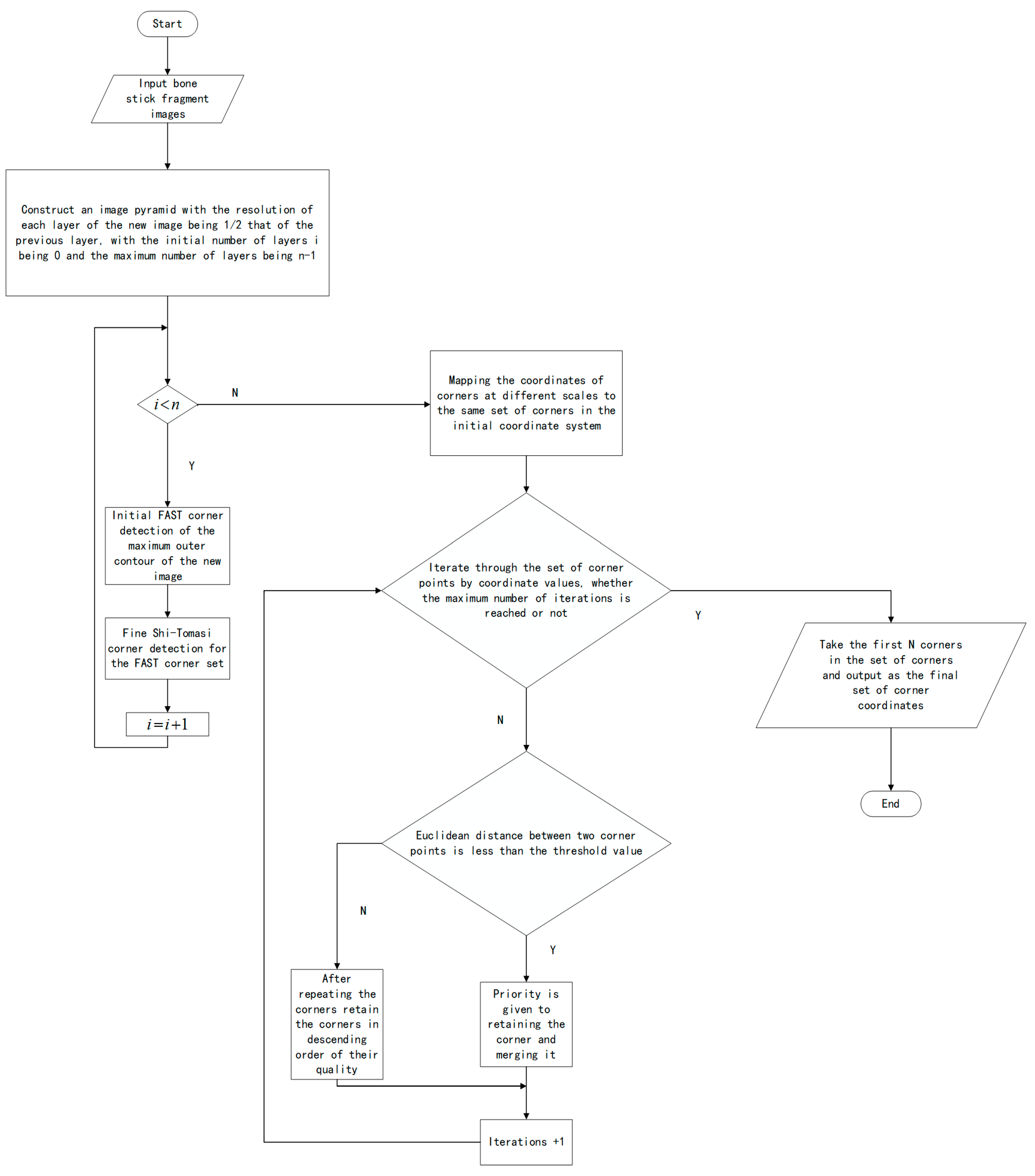
Finally, to overcome the problem that the FAST corner detection algorithm and the Shi-Tomasi corner detection algorithm are not stable at different scales, and to ensure that significant corners are stably detected in complex edges and broken areas, a multi-scale corner detection strategy is used. By constructing an image pyramid, corner detection is repeated for each level of the image, and the corners that are stably detected at multiple scales are retained. Finally, the corners are merged across scales to ensure the stability and distinctiveness of the final corner set, and the maximum outer contour features of the bone stick fragment can be represented by a smaller number of corners that are more evenly distributed.
Figure 2 shows the process of the multi-scale and multi-stage corner detection method. The specific steps are as follows:
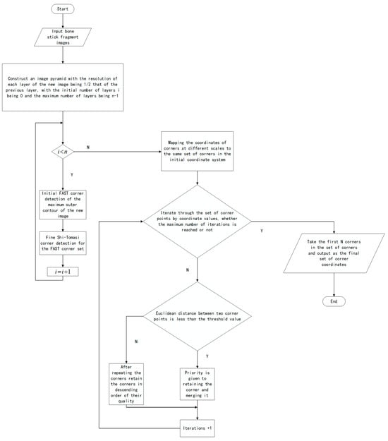
Figure 2.
Flowchart of the multi-scale and multi-stage corner detection method.
- (1)
- Image pyramid construction. Starting from the original image, the image is downsampled layer by layer to construct an image pyramid. Before each downsampling, the image is also Gaussian filtered to resist aliasing while retaining sufficiently detailed information. Assuming that the original image is , and the resolution of each level is one-half that of the previous level, then:where is the number of pyramid levels, which determines the scale coverage. The resolution downsampling factor is generally 2. This pyramid structure facilitates local corner detection at different scales.
- (2)
- Corner detection in the scale. On each scale image , the maximum outer contour of the bone stick fragment is successively subjected to Fast corner preliminary detection and Shi-Tomasi corner fine detection to obtain the corner set in this scale:where due to the differences in image information at different scales, to make detection consistent across scales, it is usually necessary to appropriately adjust the Shi-Tomasi corner response threshold so that each layer of detection has a similar number of corners and feature distributions.
- (3)
- Coordinate mapping and conversion. The coordinates of the detected corner at each scale are based on the coordinate system of the image at that scale. To merge all the corners of all scales on the original image, these coordinates need to be converted back to the original resolution. Assuming that the coordinates of the detected corner at a certain scale are , the coordinates corresponding to this coordinate at the original resolution are:where is a multiple of the downsampling factor corresponding to the scale.
- (4)
- Corner merging rules. During the merging process, if the detected corners are repeated at different scales, it is considered that these corners exhibit consistently significant characteristics at different scales, and therefore are preferentially retained. However, there may be small differences in the coordinates of the same corner after coordinate mapping, so for the judgment of duplicate corners, a distance threshold can be set. If the Euclidean distance between two corners is less than , they are considered to be the same corner:
- (5)
- Multi-scale corner merging. The set of detected corners is mapped at all scales to the coordinate system of the original image to obtain the multi-scale corner set . Then, the corner set is merged at each scale, and the maximum number of corners allowed is set to be retained to . Then, the duplicate corners are retained preferentially, and the remaining corners are retained in descending order of the Shi-Tomasi corner response value after the duplicate corners. Finally, the first corners in the merged corner set are used as the multi-scale corner set :where represents all the merged corners at multiple scales, and represents taking the top corners.
Ultimately, all the corners in the corner point set pass multi-stage detection at multiple scales. Compared with single-scale detection, the number of corners is generally slightly reduced, mainly because some non-key corners are removed. However, most of the remaining corners have high significance and stability. In addition, the number of pyramid layers and the distance threshold should not be set too large to ensure that local details are retained while avoiding excessive computational complexity and misjudgment during corner merging.
2.3. Corner Screening
To make full use of the characteristics of the broken edges of bone stick fragments, combined with the specific research samples of bone stick fragments and the actual needs of stitching, a double screening strategy based on local templates and sliding window density analysis is adopted. The corner set is optimized by combining weights, and significant corners at the broken edges are preferentially retained.
The corner screening method used mainly analyses the local curvature and corner density together to ensure that the final set of corners retained not only has significant features but also better highlights the fracture edge features of the bone stick fragments, thereby improving the priority and success rate of subsequent matching and stitching of the bone stick fragments.
The specific steps of this method are as follows:
- (1)
- Local curvature screening. For each corner in the corner set obtained by multi-scale corner detection, a fixed window centered at is set, and the significance of the corner is measured by calculating the curvature change within the window. The curvature is calculated as follows:where and represent the first derivative of the curve, and and represent the second derivative of the curve. The curve can be obtained by approximating the contour points adjacent to the point using the difference method. A threshold for the significance of the curvature is also set. If the curvature value of a corner point is less than , the corner point can be considered insignificant.
- (2)
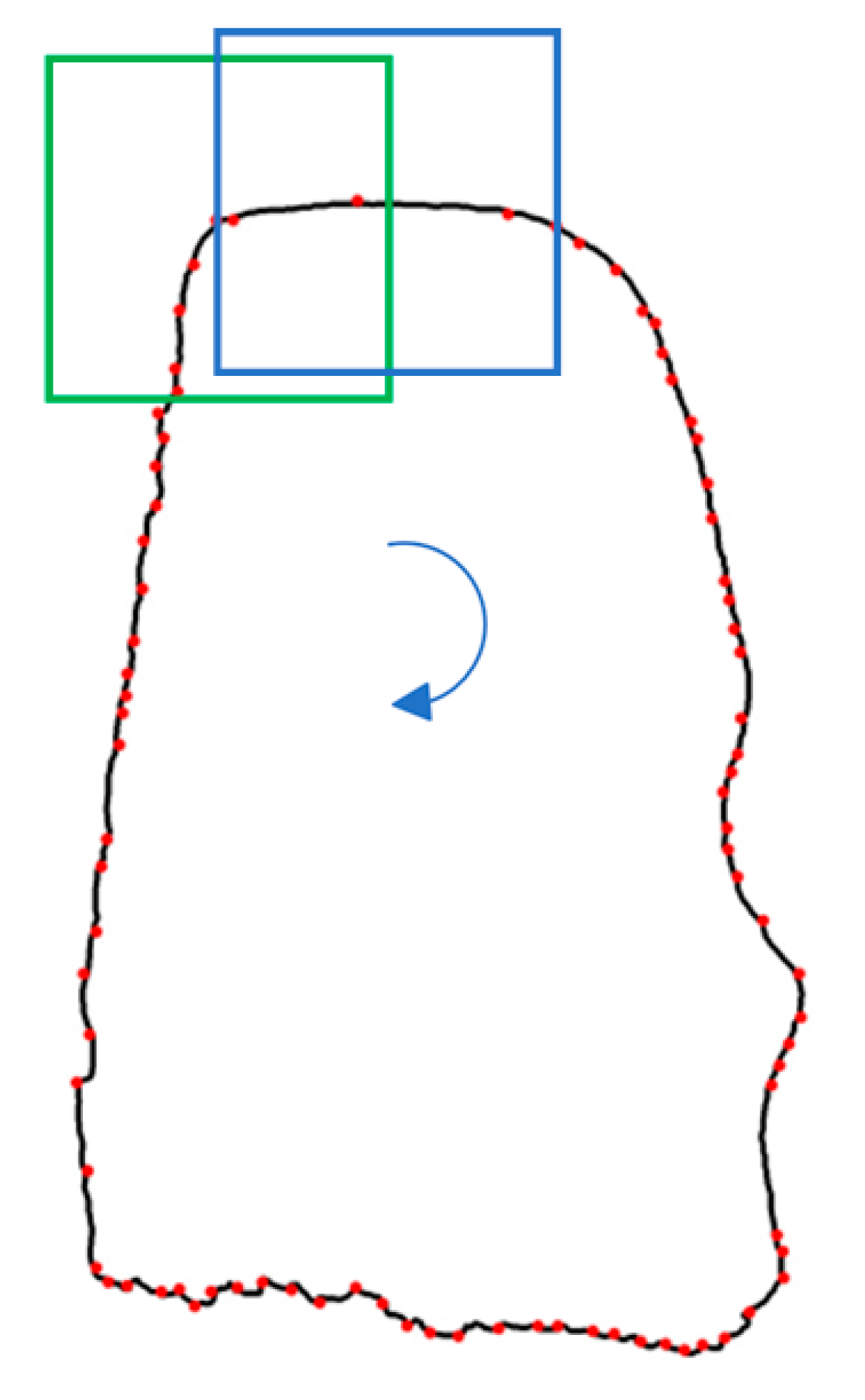
- The sliding window calculates the corner density. The length of the sliding window is set to 0.1 times the length of the maximum outer contour , i.e., , and the window movement step is set as follows . Then, starting with the initial contour point of the maximum outer contour as the center, the sliding window is moved clockwise and the number of corners are calculated in each window. The corner density function is then:where the sliding window is square, with as the window size and a value of , which prevents corners from being missed. The initial window center point is the point closest to the point on the largest outer contour. Figure 3 shows the sliding process of the sliding window on the maximum outer contour, where black represents the maximum outer contour of the bone stick fragment, red dots represent the corner marks on the maximum outer contour before screening, green squares and blue squares represent the movement trajectory of the sliding window, and arrows indicate the sliding direction is clockwise. The density threshold is also set. If the corner density in the window satisfies , the area is considered to have a high corner density and is a possible broken edge area.
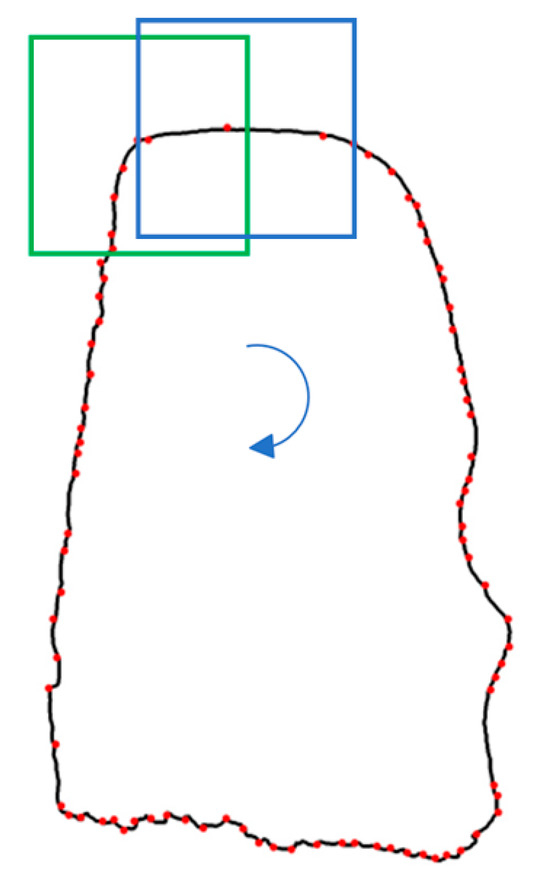 Figure 3. Sliding window sliding process.
 - (3)
- Joint screening. To ensure that the final set of corners accurately reflects the characteristics of the broken edges, each corner needs to be jointly screened. For each corner , if the curvature value , but the corner is located in a window with higher density, that is, if , then the corner is retained; otherwise, it is removed. This combined corner screening ensures that, as far as possible, corners on broken edges are retained preferentially, while corners on other edges with lower curvature values are eliminated. At the same time, regions with a higher density are identified, and all corners in these regions are marked as broken edge corners to form the broken edge set .
- (4)
- Determine the final set of corners. Priority is given to corner set in the broken edge area to ensure that there are as many prominent corners on the broken edge as possible during subsequent stitching. The maximum number of corners to be retained is set as to highlight the corner features of the broken edge, while avoiding the final corner set and the number of corners in the middle being too small, which will affect the subsequent matching process. That is, if the sum of the corners in the broken edge area and the corners retained on other edges is less than , then the corners are selected from the other edges in descending order of curvature to make up the difference, until the maximum number of corners to be retained is reached. If this is the case, the corners are sorted directly according to their curvature values, and the top corners are taken as the final corner set. After the final corner set is determined, the corner density of each window is calculated using a sliding window, and the windows are sorted in descending order of corner density to form a set of broken edge markers . Finally, the final corner set and the set of broken edge markers are output.
3. Corner-Based Bone Stick Fragment Stitching Method
Based on the results of the corner detection of the maximum outer contour of the bone stick fragment, this paper proposes a corner-based bone stick fragment stitching method, which makes full use of the dense feature area of the broken edge to improve the success rate of bone stick fragment stitching and to achieve accurate bone stick fragment stitching and recovery. The specific steps include maximum outer contour segmentation, multi-dimensional corner feature sequence matching, and fragment stitching.
3.1. Maximum Outer Contour Division
A region-based method is used to divide the maximum outer contour of the bone stick fragment into a sequence of corner points of the contour segments so that the features of the broken edges can be used more effectively for matching and stitching in the subsequent processes.
In the previous section, the set of obtained corners was sorted by corner quality. However, for stitching bone stick fragments, sorting by quality alone does not reflect the positional relationship between the corner points of the broken edges of the bone stick fragments well, and cannot be directly used to represent the contour characteristics of the bone stick fragments. If the contour points and corners of the bone stick fragments are compared one by one and the corner point sequence is rearranged, the computational complexity is too high. Therefore, in this paper, the maximum outer contour is divided into multiple contour segments using a region division method, and a sequence of corner points in a certain order is used to represent it. Combining the information about the densest and less dense regions in the obtained set of fracture edge markers, the contour segments are prioritized, so that in the subsequent matching process, the contour segments of suspected fracture edges can be matched preferentially, improving the accuracy and success rate of stitching.
Combining the shape of the bone stick fragment and the characteristics of the fracture edge distribution, the maximum outer contour is first divided into four contour segments: upper, lower, left, and right. Then, the matching priority order is determined based on the degree of overlap between the densest and less dense regions and the contour segments. The specific steps are as follows:
- (1)
- The mean and median of the corner coordinates are calculated. For all the corners in the corner set, the mean and median of the abscissa and ordinate are calculated, respectively, denoted as , , and . Then, the corner set is sorted in ascending order of the ordinate , or in ascending order of the abscissa if the ordinates are the same. The formulas for calculating the values are as follows:where represents the total number of corners.
- (2)
- The sequence of corner points of the upper contour segment is obtained. The top-left corner of the corner set is used as the initial search point and searching is started to the right. If the ordinate of the current corner point is less than the mean and median , the corner point is added to the upper contour segment corner point sequence and is set as the new search point. Searching to the right continues until no corner point meets the conditions.
- (3)
- The sequence of corner points of the lower contour segment is obtained. The bottom-left corner in the corner set is found to be the initial search point and searching is started to the right. If the ordinate of the current corner point is greater than the mean and median , the corner point is added to the sequence of corner points of the lower contour segment and is set as the new search point. Searching to the right continues until no corner point that meets the conditions remains.
- (4)
- The sequences of corner points of the left and right profile segments are obtained. After obtaining the upper and lower profile segments, their corner points are removed from the original set of corner points, and then the remaining corner points are sorted by the ordinate and the set of remaining corner points are traversed: if the abscissa of the current corner point is less than the mean and median , it is added to the left profile segment corner point sequence ; otherwise, it is added to the right profile segment corner point sequence .
- (5)
- Match priority ranking. The degree of overlap between each contour segment and the corner points of the area with the highest and second-highest concentrations of broken edges is calculated. The contour segment with the highest degree of overlap with the area with the highest concentration is selected as the priority match object, followed by the contour segment with the highest degree of overlap with the area with the second highest concentration, and finally the remaining two contour segments are matched. The degree of overlap calculation formula is:where represents the set of corners of a contour segment, such as the upper contour segment , and represents the set of corners of the densest or next densest area.
3.2. Multi-Dimensional Corner Feature Sequence Matching
3.2.1. Multi-Dimensional Corner Feature Sequence Transformation
Since different bone stick fragments are located in different coordinate systems, to accurately match the contour segments of the bone stick fragments, this paper describes the corner sequence using three geometric features:
- (1)
- Normalized chord length. First, the Euclidean distance between adjacent corner points is calculated to obtain a sequence of chord lengths, which is then normalized to minimize the effect of errors during capture. For a contour segment with corner points and an associated sequence of chord lengths, the normalized chord length is:where denotes the length of the chord between the adjacent corner points, and denotes the total length of the chord between all adjacent corner points in the contour segment.
- (2)
- Adjacent angle. The adjacent angle is used to describe the trend of change between three consecutive corner points. The angle characteristics are obtained by calculating the included angle of the triangle formed by the three corner points. The specific formula is:where indicates the angle adjacent to the corner, and are the Euclidean distances from the corner to the two adjacent corners, and is the Euclidean distance between these two adjacent corners.
- (3)
- Rate of change in distance. The rate of change in distance is used to describe the trend of change between neighboring string lengths and is defined as the ratio of the difference between neighboring string lengths to the original string length:where denotes the rate of change in distance corresponding to the corner, denotes the length of the chord between the neighboring corners, and denotes the length of the chord between the neighboring corners.
3.2.2. Longest Common Subsequence Matching Algorithm
The Longest Common Subsequence (LCS) matching algorithm, based on multi-dimensional corner feature sequences, is used to match the similarity of the contour segments of different bone stick fragments through the following steps:
- (1)
- Corner feature sequence construction. For the contour segments to be matched, the corner sequences of the contour segments are transformed into multi-dimensional corner feature sequences, including normalized chord length, neighbor angle, and distance change rate, using the method in Section 3.2.1.
- (2)
- LCS matching based on dynamic planning [19]. The different corner feature sequences of the sequence to be matched are computed separately using the dynamic planning method. Firstly, the dynamic planning table is created to store the longest matching length of each stage with size , and are the lengths of the two corner feature sequences, and the boundary value of is set to 0. Then, the dynamic planning table is updated by using the state transfer equation:where and are the multi-dimensional corner feature sequences of the contour segments to be matched, respectively, and represents the different feature types. is the dynamic threshold of each feature, where the threshold value of the normalized chord length is 0.2 times the average normalized chord length, the threshold value of the adjacency angle is 0.15 times the average angular value, the threshold value of the distance change rate is 0.15 times the average change rate, and the different corner feature sequences are computed according to their thresholds to calculate the corresponding LCS, respectively.
- (3)
- Backtracking to find the matching segment. Backtracking starts from the end of the dynamic planning table. If the condition is satisfied, it means that the and features match, so the LCS matching segment is joined, and backtracking moves to the previous row and column; otherwise, the direction that makes the value larger is chosen to backtrack until it returns to the boundary of the dynamic planning table; finally, backtracking is then conducted according to the index of the LCS matching segment to find out the matching segment of the corner sequence and to determine the matching corner pairs.
- (4)
- Merge matching segments. After obtaining the matching segments and matching corner pairs of different feature corner sequences, to better meet the subsequent stitching requirements, the matching segments are merged with the normalized chord length as the main feature, and the adjacency angle and distance change rate as the secondary features. If the matching corner pair that exists in both the adjacency angle and distance change rate matching segment does not exist in the normalized chord length corner sequence matching segment, the corner pair is added into the normalized chord length corner sequence matching segment and the matching corner pair, and the normalized chord length corner sequence matching segment and the matching corner pair at this time is the final result.
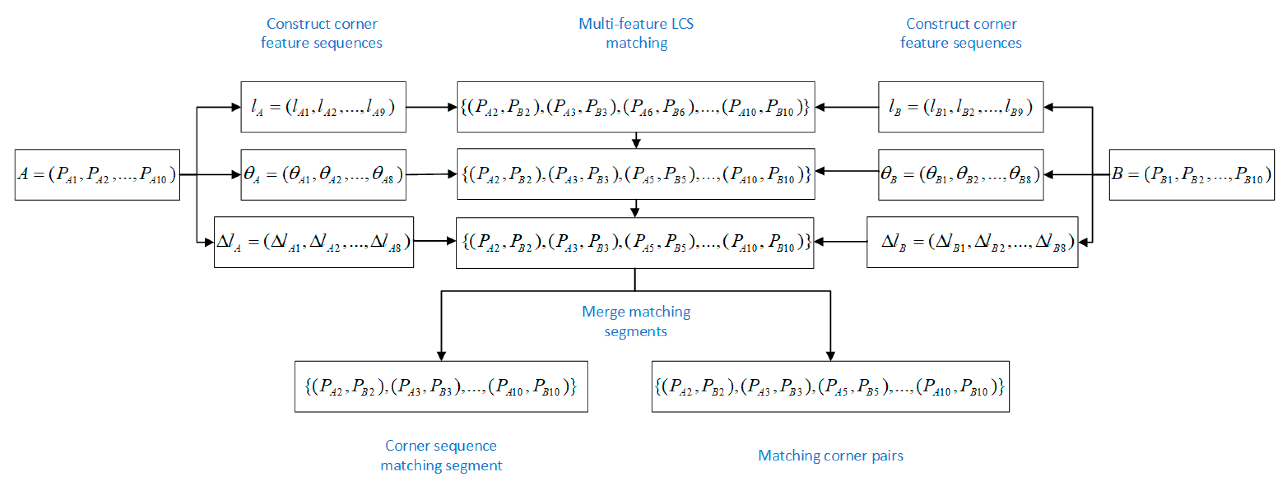
Assuming the existence of contour segment corner point sequences and which are both of a length of 10, the longest common subsequence (LCS) matching is performed on them, and Figure 4 visualizes the whole process of matching. Firstly, the construction of corner feature sequences is carried out, followed by the LCS matching of multiple feature sequences separately, and finally, the matching results are merged. It can be seen that the adjacency angle and the distance change rate as secondary features have one more pair of matching corner points compared to the normalized chord length, so the final number of matching corner point pairs is 8 pairs, and the length of the matching segment of the corner sequence is 9.
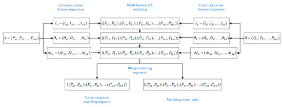
Figure 4.
LCS matching process.
3.2.3. Priority Matching Strategy
When stitching bone stick fragments together, the accuracy of the matching directly affects the stitching result. In order to minimize mismatches and improve the validity of the stitching result, a priority matching strategy is used in the matching process. The contour segments after maximum outer contour segmentation are prioritized, and the densest segments are matched first and are gradually expanded to other contour segments until the matching requirements are met. Assuming that the combination to be matched contains Fragments 1 and 2, Figure 5 shows the priority matching process. The specific steps are as follows:
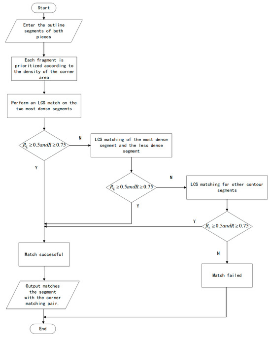
Figure 5.
Priority matching flowchart.
- (1)
- Priority division of contour segments. For Fragments 1 and 2, the maximum outer contour is divided using the method in Section 3.1, and the four contour segments are sorted into a descending contour segment set according to the degree of overlap with the densest and less dense regions. is the densest segment of the fragment and is matched with priority.
- (2)
- Match the densest segments first. For the densest segments and of Fragments 1 and 2, the LCS algorithm in Section 3.2.2 is used to match them, obtain the matched segment and matched corner pairs, and calculate the proportion of matched points and the average matching rate :where is the number of matching corners; and are the lengths of the matching profile segments at this time for Fragment 1 and Fragment 2, respectively; and and are the lengths of the matching segments for Fragment 1 and Fragment 2, respectively.
Combining the requirements of the final stitching effect, if the conditions of the proportion of matching points and the average matching rate are met, the matching is considered successful; if not, the next step of matching is entered.
- (3)
- The most intensive segment is matched with the less intensive segment. If and do not meet the matching requirements, and , and , and and are matched, respectively, and their RLs are calculated, respectively. The matching requirements in (2) are verified one by one in descending order. If the current meets the matching requirements, the matching is successful and the matching stops; if not, the next step of matching is performed.
- (4)
- Match other contour segments. The combinations in the contour segments of Fragment 1 and Fragment 2 that have not been matched are matched, their are calculated separately, and it is verified whether the matching requirements in (2) are met in descending order, one by one. If and the current meet the matching requirements, the match is successful; if none of the combinations meet the matching requirements, Fragment 1 and Fragment 2 fail to match.
3.3. Fragment Stitching
When stitching bone stick fragments, a fragment stitching method based on matching segments is used. Since the two fragments are in different image coordinate systems, it is necessary to first perform a coordinate system transformation, and then to stitch the fragments by fixing one fragment in place and translating and rotating the other fragment. The relative amounts of translation and rotation are calculated using the matching corner points of the matching segments between the fragments [20,21]. The specific steps are as follows:
- (1)
- A coordinate system is established through matching segments. If fragment and fragment are matched, the relative positional relationship between fragment and fragment can be determined through the outline segment to which the matching segment belongs. For example, if the lower outline segment of fragment matches the upper outline segment of fragment , the original images of fragment and fragment are stitched together, with the fragment remaining unchanged as the standard coordinate system for all points, and the abscissa of all points belonging to fragment remaining unchanged while the ordinate becomes twice as large.
- (2)
- Match the segment alignment by rotating and translating. After the coordinate system is established, assuming that the matching segment starts at point and ends at point on fragment , and starts at point and ends at point on fragment , two vectors can be defined:
Using the relationship between these two vectors, the rotation angle can be calculated, and the rotation matrix can be constructed:
The rotation matrix is applied to all of the contour points of fragment and it is rotated about the center of rotation, matching the start point of segment to obtain the new coordinates of all the contour points of fragment :
Then, by calculating the average translation increment between all matching corner pairs, the translation matrix is constructed:
where is the average translation increment in the X-axis direction, and is the average translation increment in the Y-axis direction.
The translation matrix is applied to all contour points after the rotation of fragment to align all matching corner pairs after fragments and are stitched.
- (3)
- Error minimization adjustment. After stitching is complete, a simple error minimization adjustment is used to further improve the stitching accuracy and optimize the stitching result. Assuming that after matching the corner pairs, and are the corresponding corner coordinates in the matching corner pair of the current fragment and fragment , respectively, the error function of the matching segment is defined to represent the sum of the Euclidean distances between all corresponding corner pairs on the matching segment:
To minimize the stitching error, the error function is reduced by performing a small translation adjustment on all contour points of the fragment until the error reaches a preset threshold or cannot be reduced any further, ensuring that the stitching result achieves a relatively optimal alignment effect.
Finally, to ensure that the overall resolution and the coordinate system of the image before and after stitching are consistent, the original coordinate system of the fragment is retained, and the coordinate system expanded in (1) is removed, so that subsequent results can be better checked and evaluated.
4. Experimental Results and Analysis
4.1. Experimental Setup and Evaluation Criteria
4.1.1. Source of Experimental Data
The experimental data used in this paper are all from the fragments of bone picks unearthed from the ruins of the Han Dynasty’s Chang’an City No. 3 in Weiyang Palace. They were photographed by professionals from the Institute of Archaeology of the Chinese Academy of Social Sciences using high-resolution imaging equipment under uniform lighting conditions. During the data collection process, a non-wide-angle camera with the same resolution and focal length was used to minimize the interference of external factors on the experimental results, ensure the accuracy and consistency of the collected data, and provide a reliable basis for experimental verification. The resolution of the experimental images is 2834 × 3780.
4.1.2. Experimental Platform Configuration
All experiments were conducted on a computing platform with the following specifications:
Hardware: AMD Ryzen7 4800H processor (2.9 GHz base frequency; AMD, Santa Clara, CA, USA) running Windows 10 64-bit operating system.
Software: Python 3.8.6 programming language with OpenCV 4.2.0.32 and NumPy 1.24.4 libraries.
4.1.3. Experimental Evaluation Criteria
To better evaluate the effectiveness of the algorithm in this paper, a subjective and objective combined method is used to evaluate the effectiveness of the algorithm based on the characteristics of the bone stick fragment samples to make a more comprehensive comparison with other algorithms.
The objective evaluation indicators are all calculated based on the maximum outer contour of the bone stick fragment, and the position of the contour in the image is fixed before evaluation. These indicators are Fracture Edge Corner Coverage (FECC), Area Similarity (AS), Center Offset Distance (COD), Shape Similarity (SS), and Comprehensive Weighted Similarity (CWS).
FECC is used to measure the ratio of the number of corners on a broken edge to the total number of corners to evaluate the effectiveness of corner detection methods for strengthening the effect of broken edges. It is defined as follows:
where indicates the number of corners on the broken edge, and indicates the number of all corner detections on the largest outer contour of the entire bone stick fragment.
AS is used to evaluate the degree of overlap between the contour after stitching and the smallest positive outer rectangle of the contour manually stitched by an expert, and is defined as follows:
where and represent the minimum positive area of the outer rectangle of the target contour and the algorithm-stitched contour, respectively. The value of AS ranges from [0, 1]. The closer the value of AS is to 1, the stronger the similarity.
COD measures the distance between the centroid of the stitched contour and that of the contour manually stitched by an expert. It reflects the deviation between the algorithm and the expert stitching results, and is defined as follows:
where (, ) and (, ) represent the centroid coordinates of the target contour and the algorithm stitching contour, respectively; E is the maximum allowable offset distance; and the COD value ranges from [0, 1], with a value closer to 1 indicating a smaller stitching offset error.
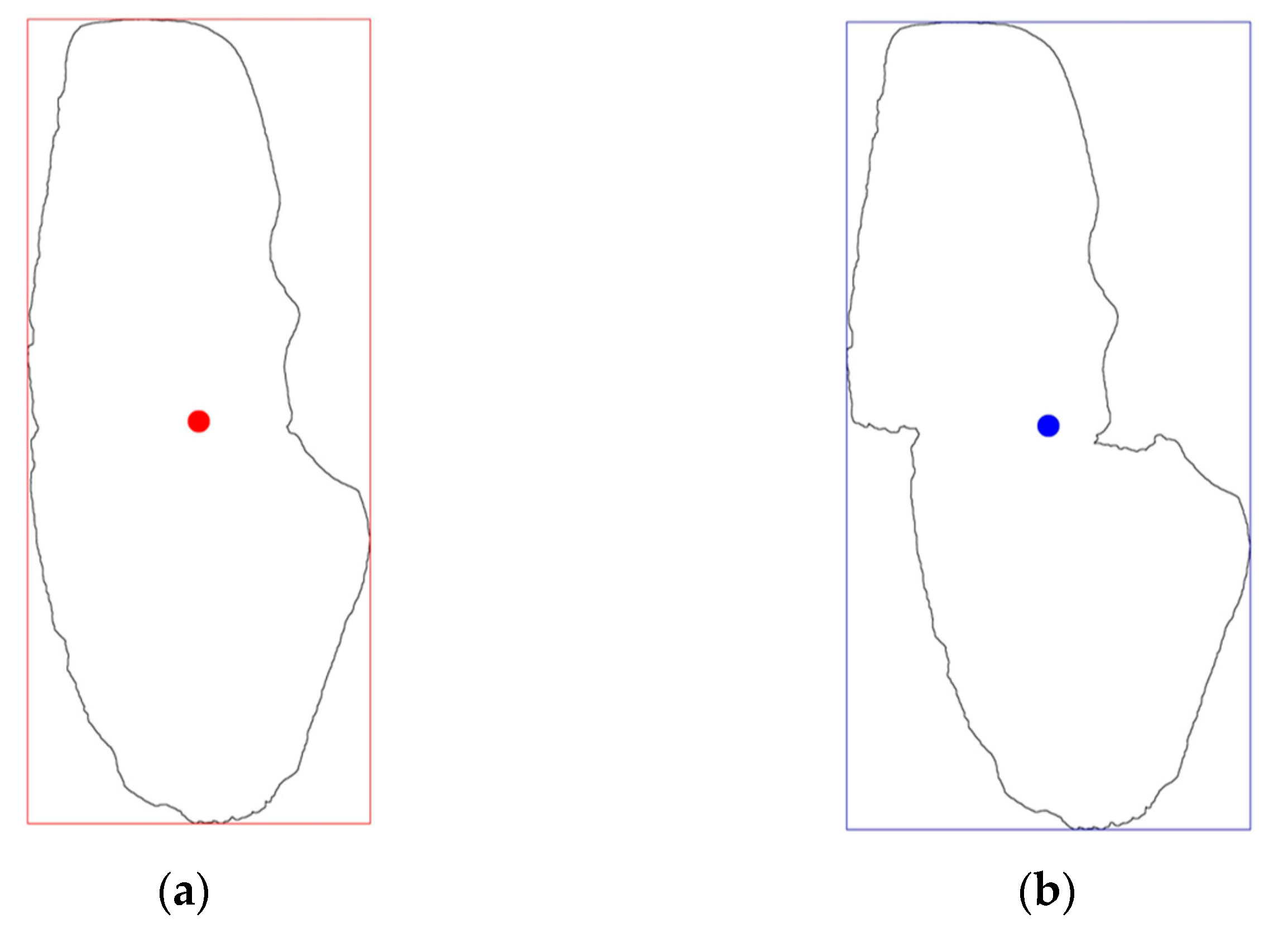
Figure 6 shows the minimum positive outer rectangle and the center of gravity. Figure 6a shows the target contour, and Figure 6b shows the algorithm-stitched contour. Taking these two contours as examples, AS is the ratio of the area of the smaller rectangle to the area of the larger rectangle in the two minimum positive outer rectangles in the calculation diagram, and COD is the offset distance error between the two marker circle coordinates in the calculation diagram.
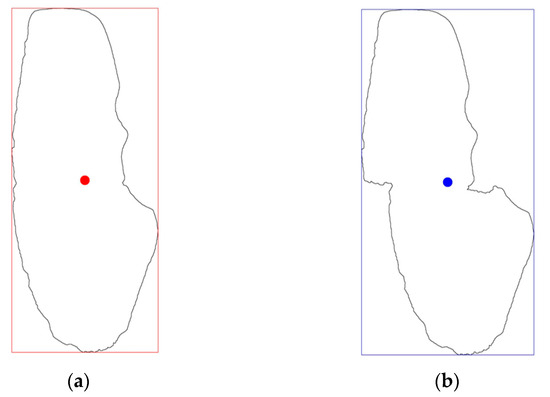
Figure 6.
Minimum positive bounding rectangle and centroid marking diagram. (a) Target contour; (b) algorithm-stitched contour.
SS evaluates the similarity between the contours after stitching by comparing them with the manually stitched contours of an expert. This paper uses an invariant shape-matching method based on Hu moments [22], defined as follows:
where represents the matching degree between contours calculated using seven invariant feature moments through the Hu moment. A smaller value indicates smaller differences between contours. The value of SS is between [0, 1]. The closer the value is to 1, the higher the similarity.
To comprehensively measure the effectiveness of the stitching algorithm, this paper proposes CWS, which combines AS, COD, and SS, as defined below:
where the weight is 0.2, is 0.4, and is 0.4; and the value of CWS ranges from 0 to 1; the closer the value is to 1, the higher the similarity between the contour stitched by the algorithm and the contour stitched manually by the expert, and the better the effect of the stitching algorithm.
4.2. Comparison with Other Corner Detection Algorithms
The complete experimental process is demonstrated using four bone stick fragments of different shapes. First, the image of the bone stick fragment is grayed out and Canny edge detection is performed. Based on the analysis of the results of a large number of current experimental samples and commonly used parameter settings, here, the Gaussian filter kernel size is set to 5, the standard deviation is 1.4, the low threshold is 30, and the high threshold is 90. This achieves a balance between noise suppression and edge retention, and the maximum outer contour of most bone stick fragments is better connected and retained.
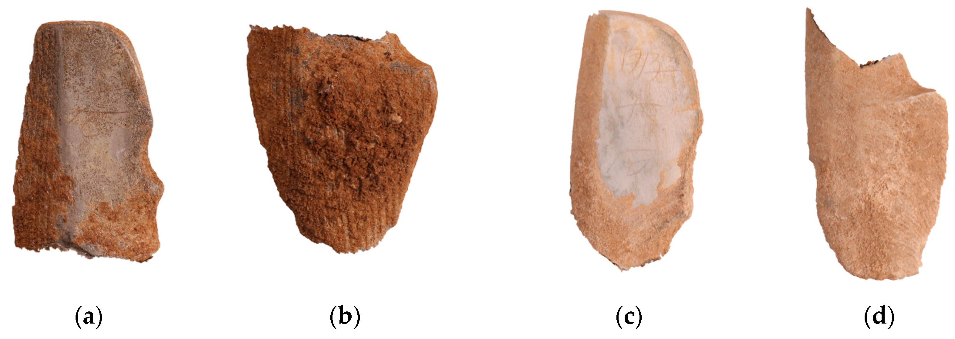
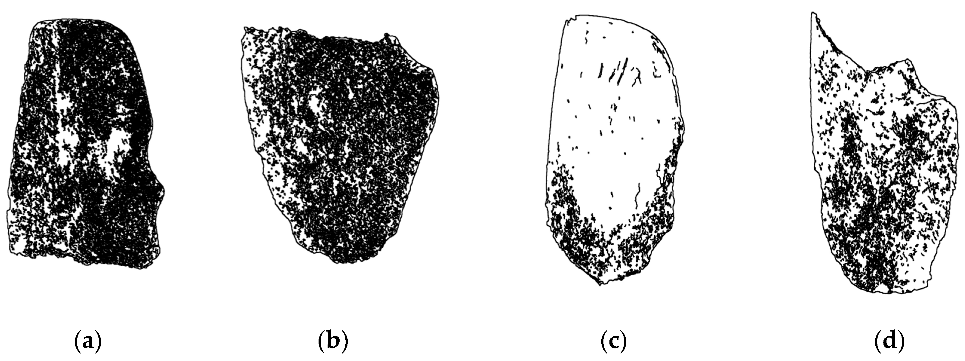
In order to better observe the edge contour, the contour information is set to black and the rest is white. Then, the maximum outer contour of the bone stick fragment is obtained using the maximum outer contour acquisition method based on the Suzuki-Abe algorithm. Figure 7, Figure 8 and Figure 9 show the original image of the bone stick fragment, the Canny edge detection result, and the maximum outer contour map, respectively, where (a), (b), (c), and (d) represent the images of Fragments 1, 2, 3, and 4 at different stages, respectively.
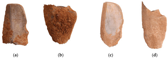
Figure 7.
Original images of bone stick fragments. (a) Fragment 1; (b) Fragment 2; (c) Fragment 3; (d) Fragment 4.

Figure 8.
Canny edge detection results. (a) Fragment 1; (b) Fragment 2; (c) Fragment 3; (d) Fragment 4.

Figure 9.
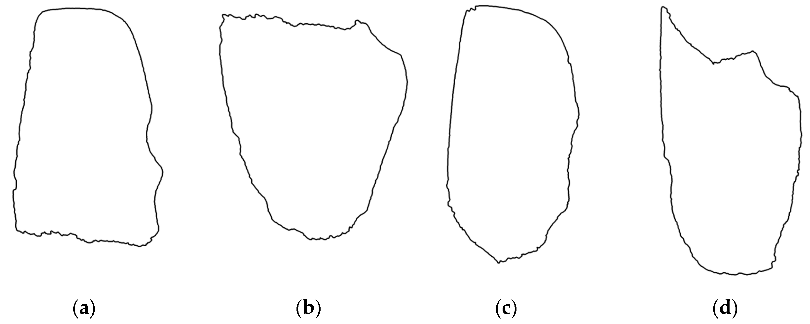
Maximum outline diagram. (a) Fragment 1; (b) Fragment 2; (c) Fragment 3; (d) Fragment 4.
After obtaining the maximum outer contour, multi-stage corner detection is performed at multiple scales. Based on the analysis of the results of a large number of current experimental samples and commonly used parameter settings, the number of pyramid layers is set to 3, and the FAST corner detection algorithm detection thresholds at different scales are 10, 16, and 30, respectively. The minimum per-pixel connectivity parameters are 9, 7, and 6, respectively. The Shi-Tomasi corner detection thresholds are 0.01 times, 0.06 times, and 0.4 times the maximum response value, respectively. The kernel size of the Gaussian filter before each downsampling is 5, and the standard deviation is 1 and 1.4. The distance threshold for repeated corner determination during corner merging is 20, and the maximum allowable number of corners to be retained is 0.9 times the number of single-scale multi-stage corner detections.
This parameter setting ensures that without excessive scale segmentation, the number of corners after FAST corner detection at a single scale for the experimental sample is 300–500, which can completely represent the maximum outer contour of the bone stick fragment. After Shi-Tomasi fine corner detection at a single scale, the number of corners is significantly reduced and more evenly distributed, and the number is about 0.25 times the number of corners after FAST corner detection. After multi-scale and multi-stage corner detection is combined, the number of corners is slightly reduced, ensuring the key corner features are present while removing some unstable pseudo-corners. The number is about 0.8 times that of multi-stage corner detection under a single scale. At this time, the distribution of corners can more accurately represent the maximum outer contour of the bone stick fragment, but it does not highlight the broken edge features of the bone stick fragment, which requires further screening.
Finally, local curvature and sliding window density analysis are used to screen the corners. Based on the analysis of the results of a large number of current experimental samples and common parameter settings, the density threshold is set to 0.8 times the average density of each window, the curvature significance threshold is set to 0.8 times the maximum curvature, and the maximum number of corners retained is set to 0.5 times the number of corners before screening. This can greatly reduce the total number of corners while enhancing the broken edge features.
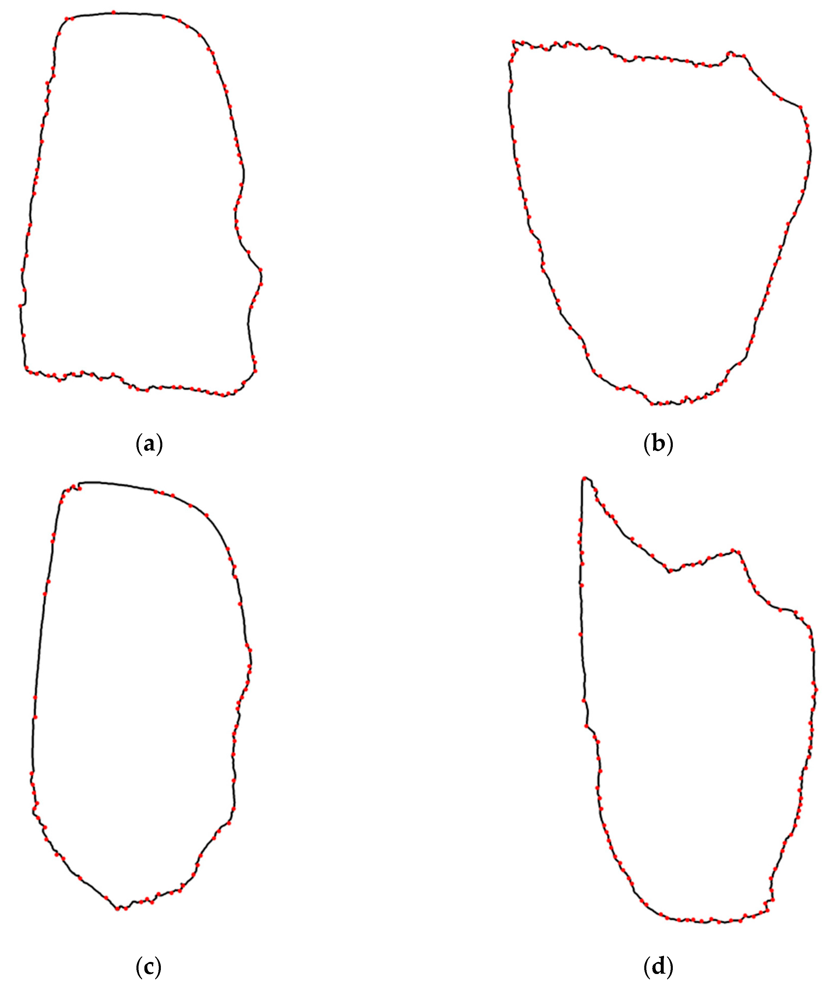
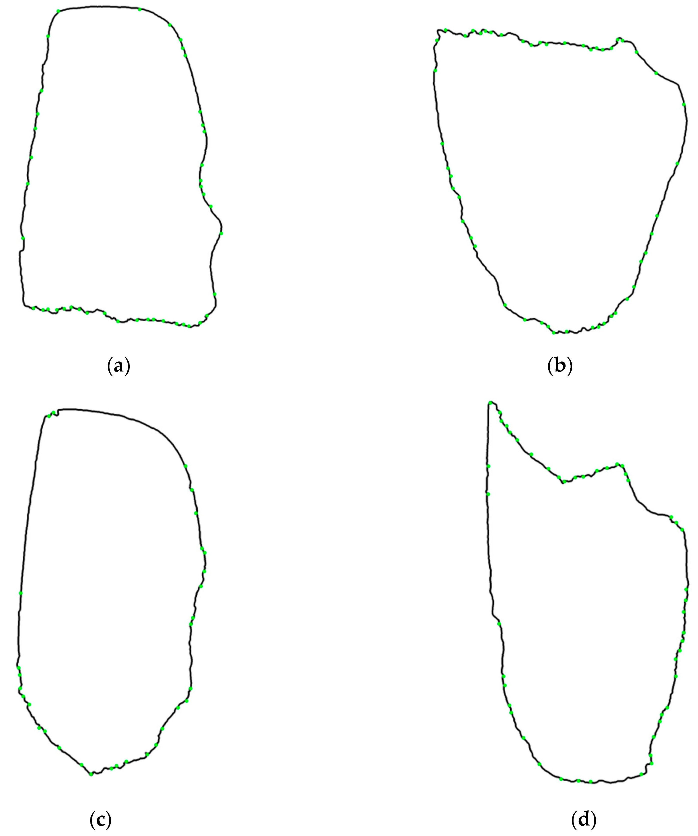
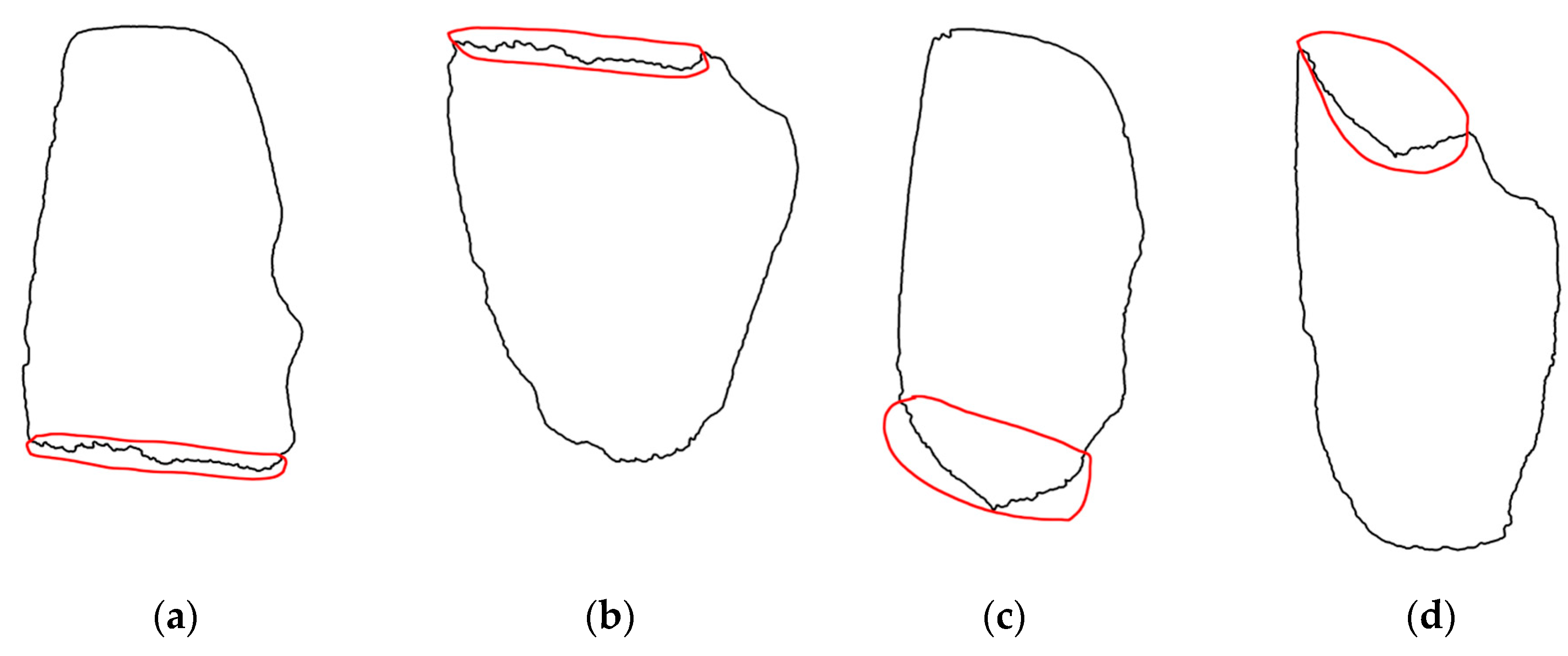
Figure 10, Figure 11 and Figure 12 show the corner detection results before screening, the corner detection results after screening, and the known fractured edges labeled by the expert, where (a), (b), (c), and (d) represent the images at different stages of Fragment 1, Fragment 2, Fragment 3, and Fragment 4, respectively. In different fragments, the red dots in Figure 10 represent the corner marks before screening, the green dots in Figure 11 represent the corner marks after screening, and the red circles in Figure 12 represent the fracture edges marked by experts. Table 1 shows the number of corners before and after screening, as well as the FECC.
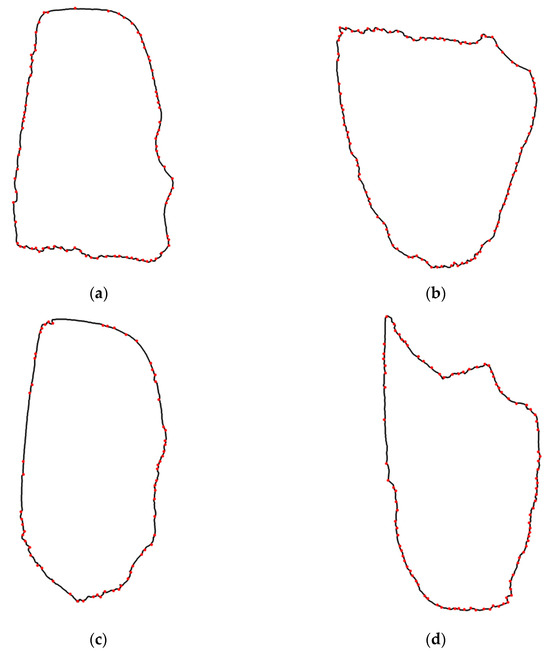
Figure 10.
Screening of pre-corner detection results. (a) Fragment 1; (b) Fragment 2; (c) Fragment 3; (d) Fragment 4.
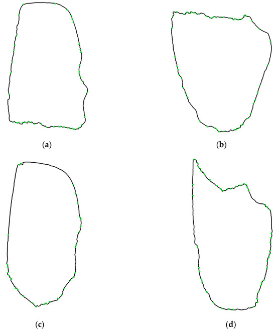
Figure 11.
Corner detection results after screening. (a) Fragment 1; (b) Fragment 2; (c) Fragment 3; (d) Fragment 4.

Figure 12.
Known fracture margins marked by experts. (a) Fragment 1; (b) Fragment 2; (c) Fragment 3; (d) Fragment 4.

Table 1.
The number of corners before and after screening and the FECC.
Table 1 and Figure 10, Figure 11 and Figure 12 show that under the premise of ensuring the prominence and sufficient number of the corner points of the fracture edge, the corner points after screening are more densely distributed at the fracture edge than other areas, and can effectively characterize the features of the fracture edge, which can be used for subsequent stitching work. When the total number of corners after screening is close to half of the number before screening, the average FECC after screening increases by about 49.76%.
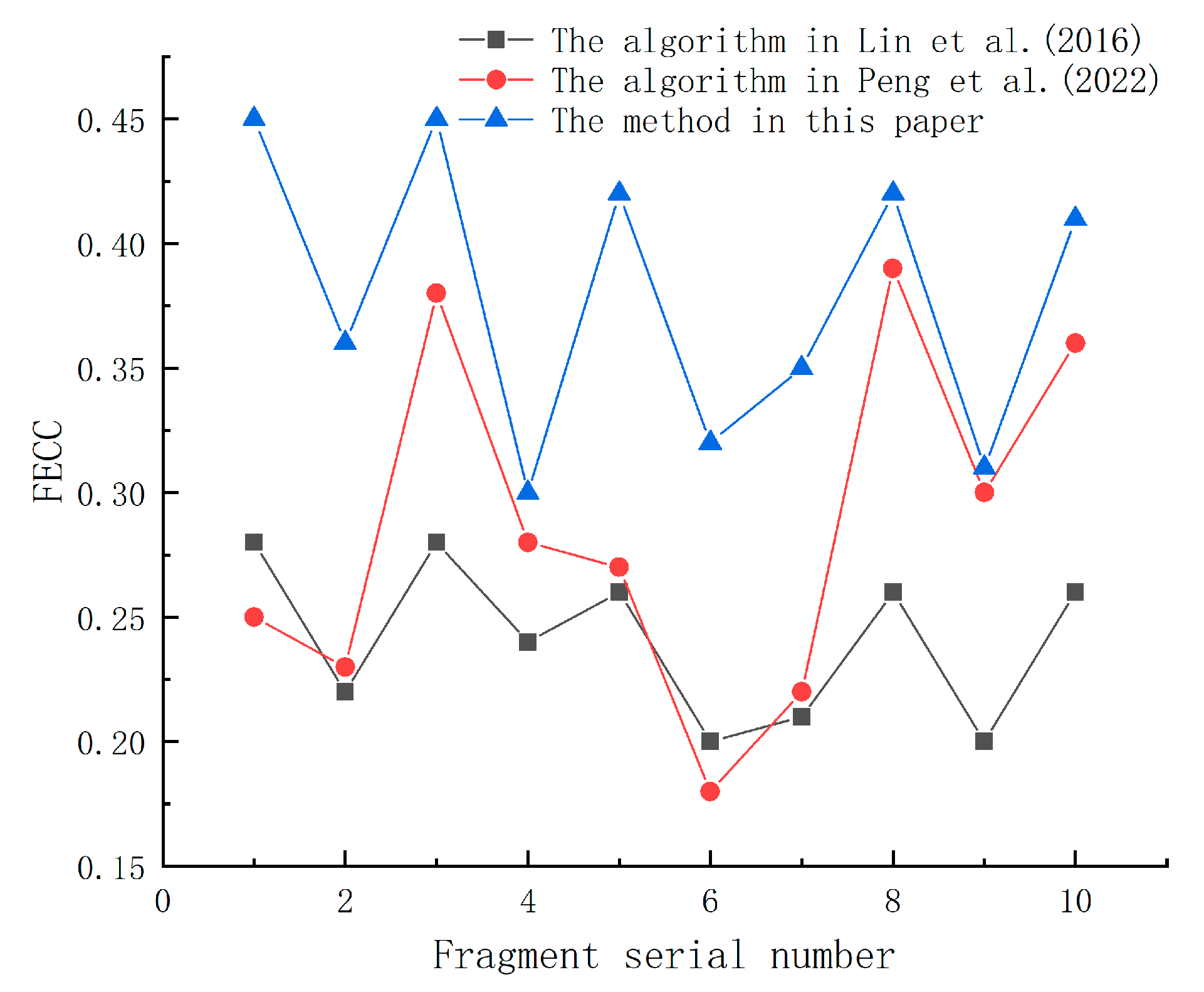
To further verify the effectiveness of the method in enhancing the features of broken edges, 10 bone stick fragments were selected for comparative experiments with the corner detection algorithms in [10,12]. Ref. [10] uses curvature to detect the corners of small bronze fragments, which are similar to the experimental samples in this paper and are also one of the classic corner detection methods. Ref. [12] is an improved Shi-Tomasi corner detection method, which can verify the enhancement effect of the method in this paper on the corner features of the broken edges well. At the same time, in order to ensure the objectivity of the experimental results, each detection algorithm only detects the largest outer contour, and tries to ensure that the corners of the broken edges are prominent and in sufficient quantity. Figure 13 shows a comparison of the FECC corner detection of different algorithms.
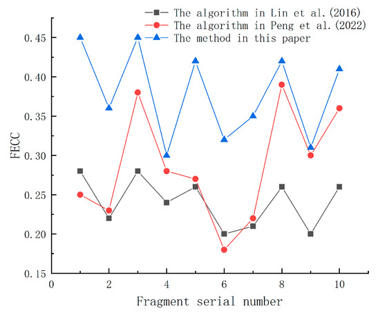
Figure 13.
Comparison of FECC with corner detection using different algorithms [10,12].
Figure 13 shows that the FECC of the algorithm in [10] is the lowest, with a value between 0.2 and 0.28 and an average FECC of 0.24; the FECC of the algorithm in [12] is between 0.18 and 0.39, with a higher upper limit than the algorithm in [10], and an average FECC of 0.29; the FECC of the method in this paper is between 0.3 and 0.45, with an average FECC of 0.38, and the FECC on each fragment sample is greater than the results of the algorithm in study [10] and the algorithm in study [12]. Compared with the algorithm in study [10], the average FECC of the method in this paper is improved by about 57.26%; compared with the algorithm in study [12], the average FECC is improved by about 32.52%, and the comprehensive average FECC is improved by about 44.89%.
The experimental results show that the algorithm in [10] extracts a large number of corners based on curvature, but most of them are redundant corners. Although local pseudo-corner removal is performed subsequently, the effect is not good, resulting in an excessive number of corners on the edges of non-fracture surfaces. The algorithm in [12] performs pseudo-corner removal after multi-scale corner detection and merging, but due to the lack of close-range corner deduplication and the lack of specific processing of the fracture edges of bone stick fragments, there is a small amount of corner clustering, while the FECC is low, and the method cannot make good use of the corner feature that protrudes from the fracture edge of the bone stick fragment. Analysis shows that the method in this paper can strengthen the fracture edge feature with higher effectiveness than other methods while ensuring the prominence and sufficient quantity of fracture edge corners.
4.3. Comparison with Other Stitching Algorithms
Fragments 1, 2, 3, and 4 from 4.2 are selected to continue the stitching experiment. They have already been stitched by the expert group, with Fragments 1 and 2 forming combination 1 and Fragments 3 and 4 forming combination 2.
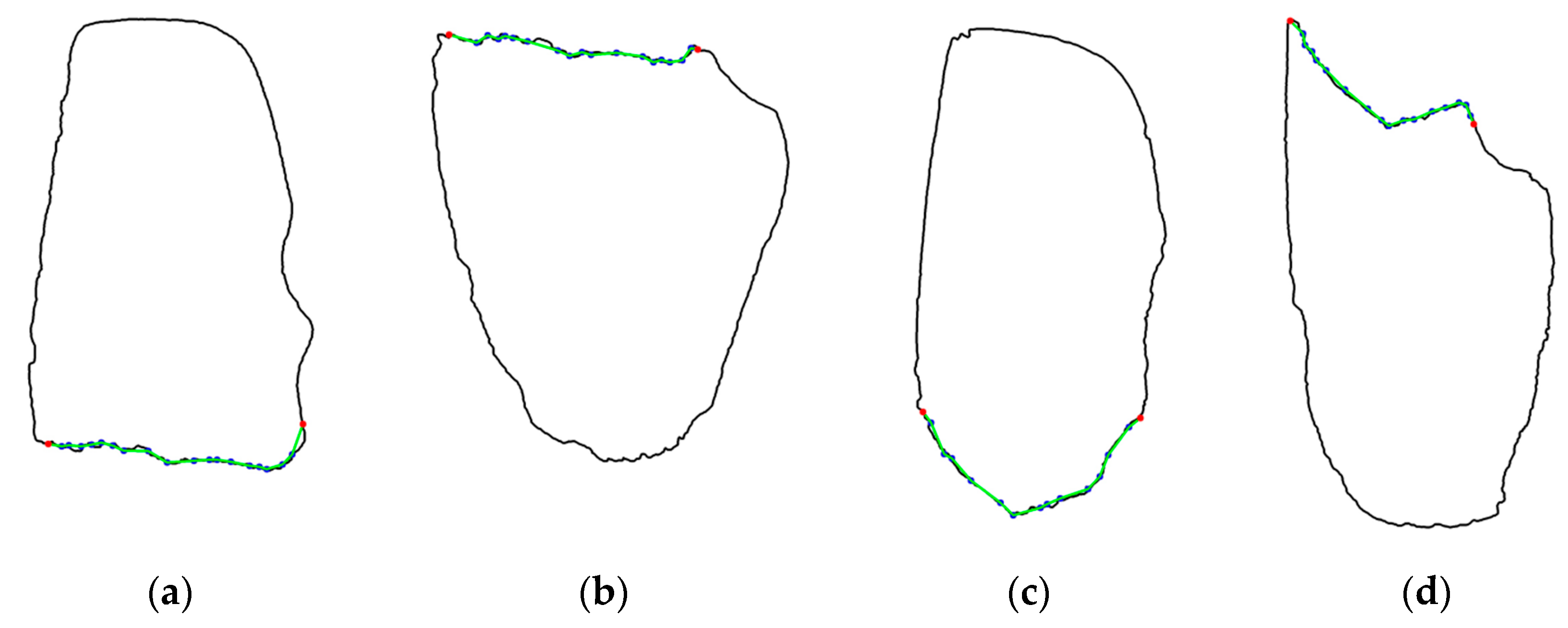
First, the maximum outer contour of the bone stick fragments is segmented based on the corner detection results using the region growing method, and the matching priorities of each contour segment are calculated. The contour segments of each fragment are numbered 1–4 in descending order of priority. Taking the densest segment as an example, Figure 14a–d show the identification diagrams of the densest segments of Fragment 1, Fragment 2, Fragment 3, and Fragment 4, denoted as 1-1, 2-1, 3-1, and 4-1, respectively. In Figure 14, the red dots in different fragments represent the starting and ending corners of the densest segment of each bone stick fragment, the blue dots represent the middle corners, and the green lines connect all the corners to represent the densest segment as a whole. It can be seen that the densest segments 1-1 and 3-1 of Fragments 1 and 3 are both lower contour segments, while the densest segments 2-1 and 4-1 of Fragments 2 and 4 are both upper contour segments.
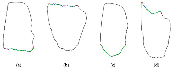
Figure 14.
Diagram marking the densest segments. (a) Fragment 1; (b) Fragment 2; (c) Fragment 3; (d) Fragment 4.
Then, the bone stick fragments in combination 1 and combination 2 are matched using a priority matching strategy based on multi-dimensional corner feature sequences. The matching results are shown in Table 2. Combinations 1-1 and 2-1 in combination 1 achieve 16 matching corner points, with a matching point ratio and an average matching rate of 0.842 and 0.889, respectively. Combinations 3-1 and 4-1 in combination 2 achieve 10 matching corner points; the matching point ratio and average matching rate both reach 0.667 and 0.788, and the matching result data all reach a high level and meet the requirements for a successful match. It can be seen that because of the enhanced broken edge feature during corner detection, both combinations complete their matching in the densest segment where the possibility of a suspected broken edge is highest. Figure 15 shows the corner matching results of the bone stick fragments in combination 1 and combination 2. For example, Figure 15a shows the corner matching diagram of the lower contour segment of Fragment 1 and the upper contour segment of Fragment 2, and Figure 15b shows the corner matching diagram of the lower contour segment of Fragment 3 and the upper contour segment of Fragment 4. In Figure 15, the red dots in different fragments represent the starting and ending corners of the densest segment of each bone stick fragment, the blue dots represent the middle corners, and the green lines connect all the corners to represent the whole densest segment. The blue connecting lines between the upper and lower fragments connect a set of matching corner pairs.
Table 2.
Fragment matching results for combination 1 and combination 2.
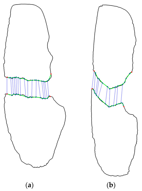
Figure 15.
Diagram of corner matching. (a) Combination 1; (b) Combination 2.
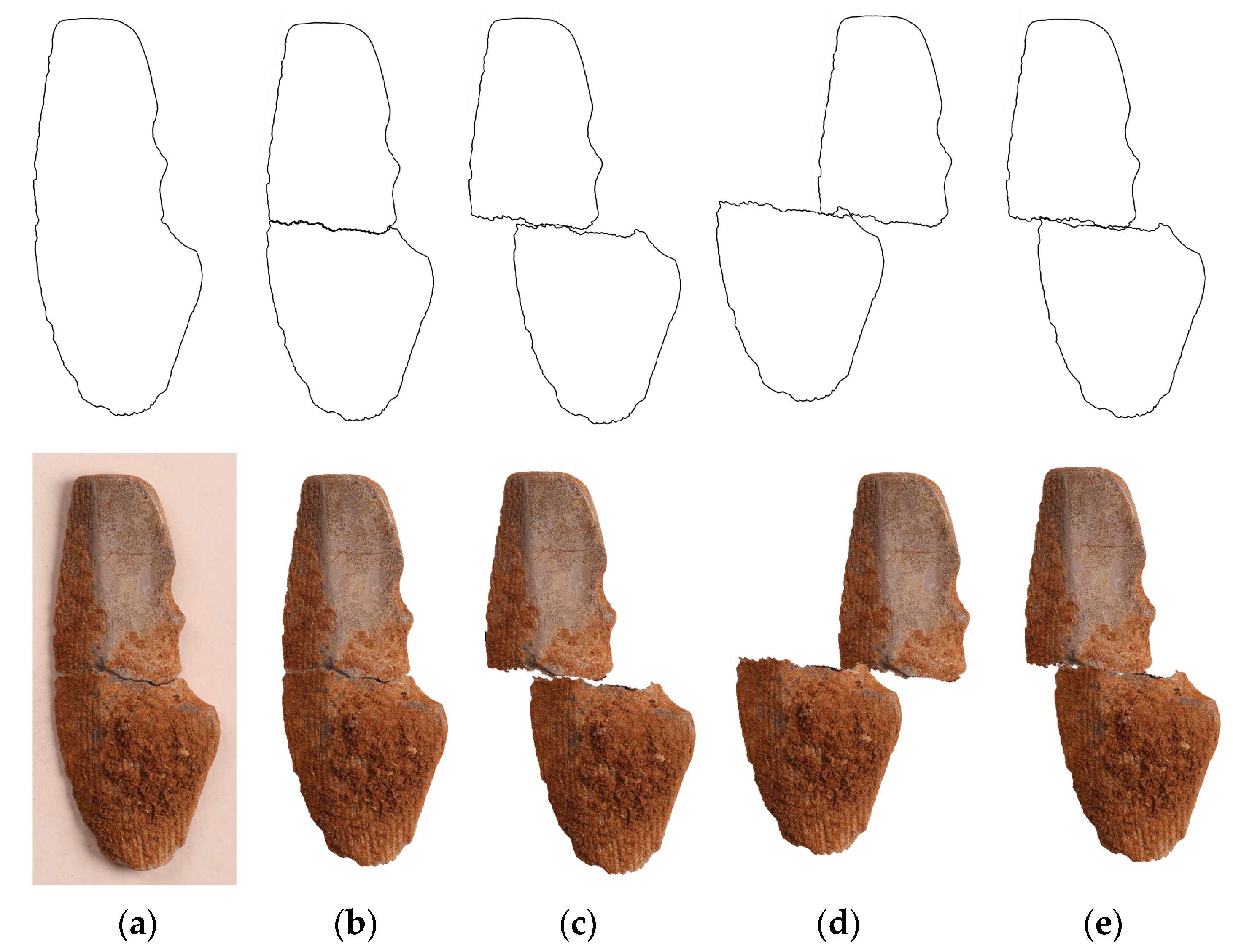
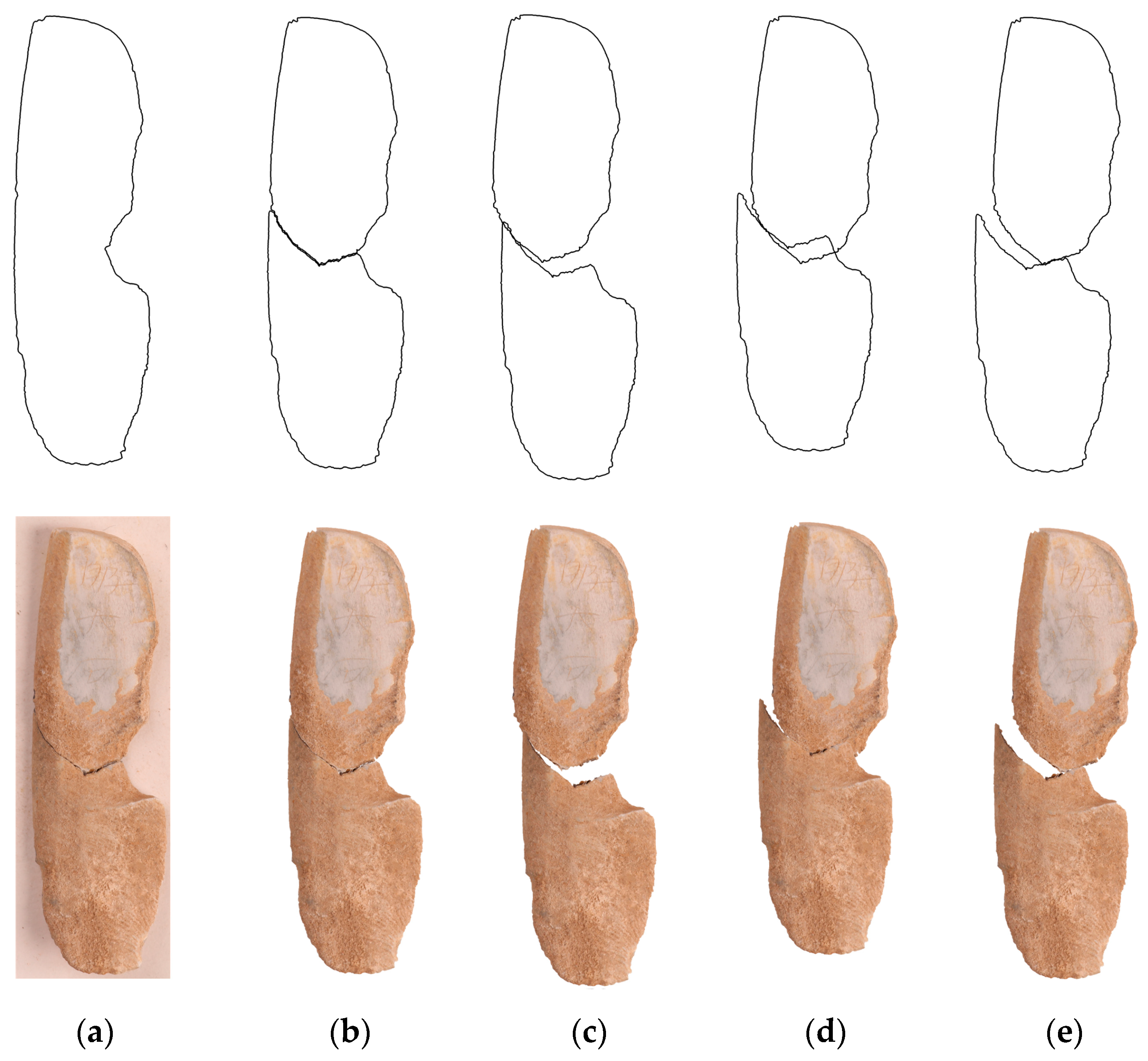
Finally, the corner detection part of the method in this paper is replaced with the corner detection algorithm in [12] (hereinafter referred to as the [12] algorithm), and it is compared with the [9] algorithm and the [10] algorithm in a comparative experiment with the method in this paper. Ref. [9] is a classic algorithm for stitching traditional cultural relic fragments, and ref. [10] uses curvature to detect the corners of small bronze fragments and then uses the longest common subsequence to stitch them together, which is similar to the experimental sample in this paper, and study [12] is an improved Shi-Tomasi corner detection method. It can verify the effect of the method in this paper on enhancing the corner features of broken edges on the accuracy of subsequent matching and stitching well. Taking the four fragments in combination 1 and combination 2 as an example, Figure 16 and Figure 17 show the results of combining the outlines of the fragments in combination 1 and combination 2 with the original images using different algorithms and the manual stitching method, respectively. Among them, Figure 16a–e and Figure 17a–e show the results of the manual stitching of the fragments in combination 1 and combination 2 by an expert, the method in this paper, the algorithm in reference [9], the algorithm in reference [10], and the algorithm in reference [12], respectively. It can be seen that the stitching results of the method in this paper are more similar to the expert’s stitching results than the stitching results of the other algorithms.
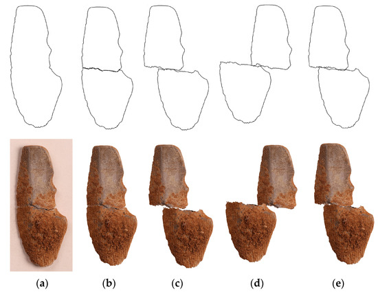
Figure 16.
Combination 1 using different algorithms and manual stitching by an expert. Fragment outlines and the results of stitching with the original image are both shown. (a) Expert manual stitching; (b) the method in this paper; (c) the algorithm in [9]; (d) the algorithm in [10]; (e) the algorithm in [12].
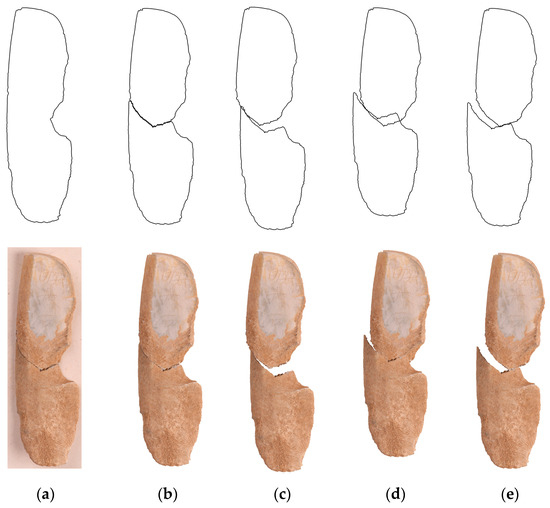
Figure 17.
Combination 2 using different algorithms and manual stitching by an expert. Fragment outlines and the results of stitching with the original image are both shown. (a) Expert manual stitching; (b) the method in this paper; (c) the algorithm in [9]; (d) the algorithm in [10]; (e) the algorithm in [12].
The experimental data comparing the results of different algorithms with the results of manual stitching by an expert are shown in Table 3. It can be seen that in combinations 1 and 2, the indicators of the method in this paper are higher than the results of other algorithms. The ASs all reached 0.98, the CODs all reached 0.93, the SSs reached 0.98 and 0.97, respectively, and the CWSs all reached 0.96. Compared with the algorithm in reference [9], the method in this paper has an average increase of about 18.08%, 129.71%, 37.41%, and 49.96% in AS, COD, SS, and CWS; they increased by an average of about 18.08%, 129.71%, 37.41%, and 49.96%, respectively, compared with the algorithm in reference [9]; compared with the algorithm in reference [10], AS, COD, SS, and CWS increased by an average of about 17.12%, 393.22%, 14.32%, and 48.03%, respectively; and compared with the algorithm in reference [12], AS, COD, SS, and CWS increased by an average of about 11.59%, 62.08%, 9.57%, and 25.75%, respectively.
Table 3.
Experimental data comparison results.
The experimental results show that the algorithm in [9] uses Freeman’s code to extract image feature information and angular edge features for matching, but the features are too singular, resulting in stitching offset errors. The algorithm in [10] uses curvature to extract contour corner points and the longest common subsequence to match the overall contour, but for bone stick fragments with more complex edges, the corner detection and matching method is not suitable, resulting in large stitching offset errors and overlap phenomena. Although the algorithm in [12] improves on the original Shi-Tomasi corner detection algorithm, it does not strengthen the screening of bone stick fracture edge features. Therefore, although it incorporates the matching and stitching parts of this paper, the input corners are of poor quality, resulting in mismatches and small stitching offset phenomena. Analysis shows that the method in this paper not only has high-quality corner input, enhanced broken edge features, and a multi-dimensional corner feature sequence matching and priority matching strategy, but it also solves the stitching offset errors and the overlap phenomena produced by other stitching algorithms, achieving better stitching results.
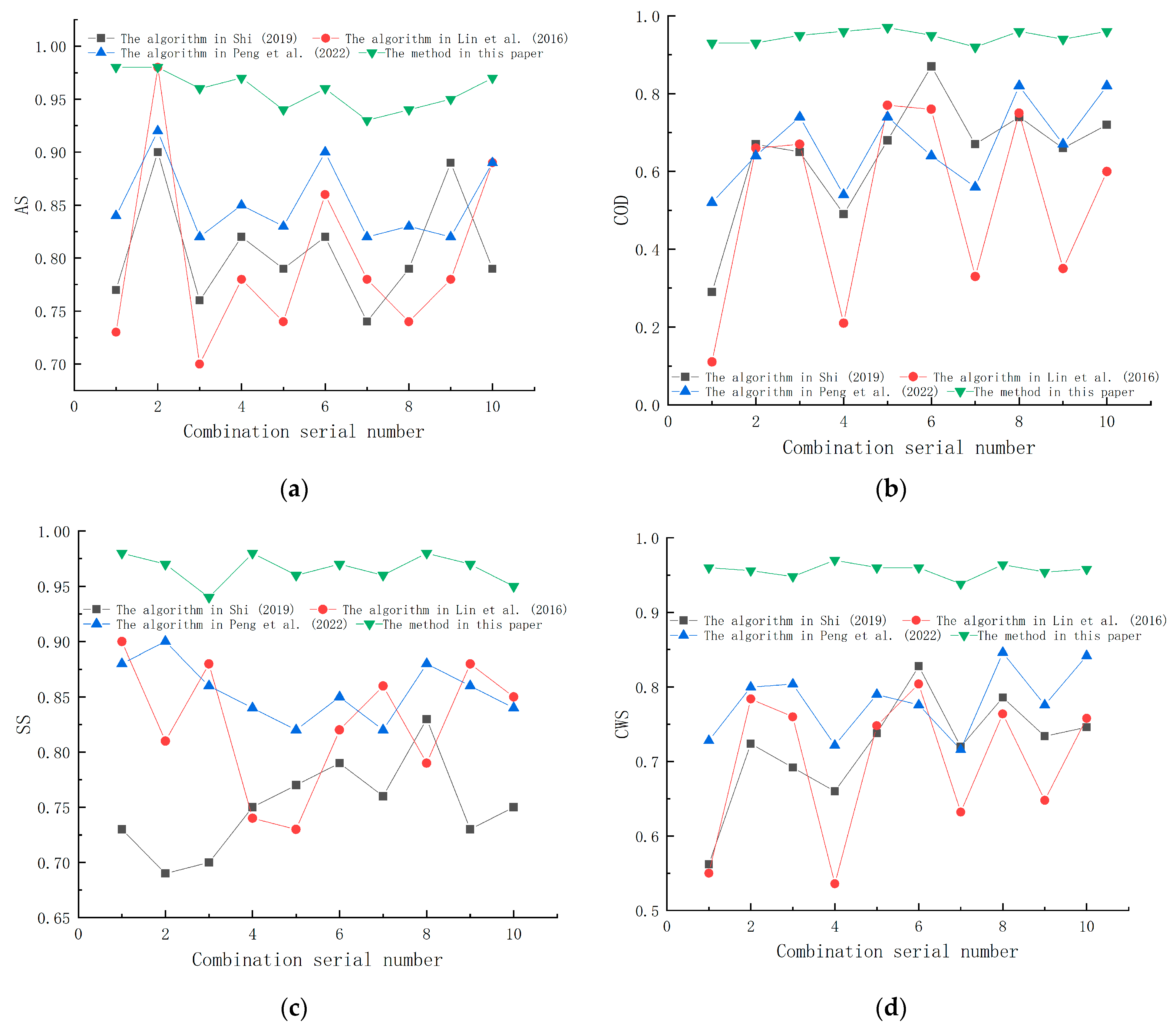
To further verify the effectiveness of the method in this paper, 10 groups of 20 bone stick fragments that have been manually stitched by experts are selected. The fragment contours are stitched using the method in this paper and other algorithms, and the results of the expert stitching are used as the standard to compare the similarity of the stitching contours. Figure 18 shows the results of the experiment.
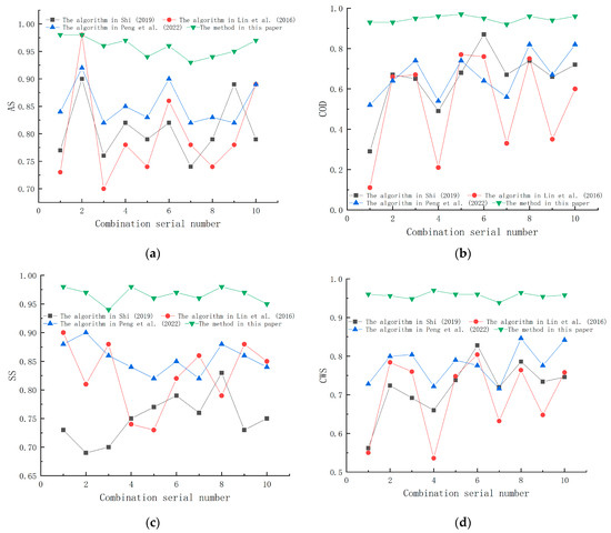
Figure 18.
Comparison of the results of stitching 10 groups of fragments [9,10,12]. (a) AS comparison; (b) COD comparison; (c) SS comparison; (d) CWS comparison.
It can be seen from Figure 18a that the AS is the highest and most stable, and compared to the algorithm in [9], the algorithm in [10], and the algorithm in [12], the AS is improved by an average of about 19.12%, 21.14%, and 12.58%, respectively. It can be seen from Figure 18b that the COD of the method in this paper is much higher than that of the other algorithms, and compared to the algorithm in [9], the algorithm in [10], and the algorithm in [12], COD is on average about 59.62%, 167.16%, and 44.86% higher, respectively. As can be seen from Figure 18c, the SS of the method in this paper is higher than that of the other algorithms. Compared to the algorithms in [9,10,12], the SS is improved by an average of about 29.11%, 17.53%, and 13.06%, respectively. As can be seen from Figure 18d, the CWS of the method in this paper is consistently higher than that of the other algorithms. Compared to the algorithms in [9,10,12], the CWS is improved by an average of about 34.42%, 39.81%, and 23.05%, respectively.
The experimental results show that compared with other algorithms, the method in this paper solves the problems of stitching offset errors and overlap, and achieves better stitching results. The average improvements in AS, COD, SS, and CWS are 17.61%, 90.55%, 19.91%, and 32.42%, respectively.
The time complexity of study [9], study [10], study [12], as well as the methods in this paper is O(n2), and the space complexity is O(n). Figure 19 shows the specific running time of each method for 10 sets of fragments, which shows that this paper’s method has a high time efficiency under the premise of ensuring a higher stitching accuracy by prioritizing the matching strategy and other methods.
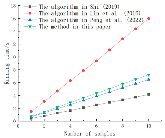
Figure 19.
Running time chart [9,10,12].
4.4. Analysis of the Universality of Stitching Methods
To verify the generality of the method in this paper, 200 groups of 400 bone stick fragments that have been manually stitched by experts are selected. The fragment contours are stitched using the method in this paper, and the results of the expert stitching are used as the standard to evaluate the CWS of the method under different sample sizes. After being determined by experts, if the value of CWS is greater than 0.9, the group of fragments is considered to have been successfully stitched. If the value of CWS is between 0.85 and 0.9, the stitching is considered to be of high quality, and if the CWS value is lower than 0.85, the stitching is considered to have failed.
Table 4 shows that when the sample size includes 50, 100, and 200 groups of fragments, the stitching success rates are 92%, 86%, and 80.5%, respectively. It can be seen that as the number of samples increases, there are bone stick fragment samples that are too complex, such as having broken edges that are too flat and fragments that are too small. The acquisition of the maximum outer contour, corner detection, and multi-dimensional corner feature sequence matching of these samples are not effective, resulting in a certain deviation error and an overlap in the stitching results, and even a failure to match, which leads to a decrease in the stitching success rate. However, the stitching success rate of 80.5% basically meets the needs of stitching bone stick fragments.
Table 4.
Results of the experiment to stitch together 200 bone stick fragments.
5. Conclusions
Given the low success rate of the existing methods for stitching bone stick fragments due to the complex edges of the fragments, this paper proposes a bone stick fragment stitching method based on improved corner detection. By combining multi-scale and multi-stage corner detection, as well as a double screening mechanism of local templates and corner density analysis, the characteristics of broken edges are effectively enhanced. After segmenting the maximum outer contour based on the corner features, a priority matching strategy is used to perform multi-dimensional priority matching of the corner feature sequences in the densest segments, which effectively improves the success rate of stitching. The experimental results show that, compared with other algorithms, the average FECC of this method is increased by about 44.89%, and the average CWS is increased by about 32.42%, which meets the needs of stitching bone stick fragments. In the future, with the increase in the number of various samples of bone stick fragments, further research needs to be conducted based on contour features in combination with other features or methods.
Author Contributions
Conceptualization, J.L. and H.W.; methodology, J.L.; software, J.L.; validation, J.L. and K.W.; formal analysis, Z.W.; investigation, T.W.; resources, R.L.; data curation, J.L. and R.L.; writing—original draft preparation, J.L.; writing—review and editing, J.L. and K.W.; visualization, J.L.; supervision, K.W., H.W. and Z.W.; project administration, H.W. and K.W.; funding acquisition, H.W. All authors have read and agreed to the published version of the manuscript.
Funding
This research was funded by the National Social Science Fund Special Project of China under grant number 20VJXT001.
Institutional Review Board Statement
This study did not require ethical approval due to not involving humans or animals.
Informed Consent Statement
Not applicable.
Data Availability Statement
The data used to support the findings of this study are part of a private image dataset.
Acknowledgments
This research was supported by experts from the Shaanxi Institute for the Preservation of Cultural Heritage, and we express our thanks for their assistance.
Conflicts of Interest
The authors declare no conflicts of interest.
References
- Qi, H. Probe into the Archives of Bone Signet in Han Dynasty. Lantai World Shenyang China 2014, 26, 58–59. [Google Scholar]
- Gao, M. The Bone Sticks of the Weiyang Palace in Chang’an City of Han Dynasty (9 Rules). J. Bohai Univ. (Philos. Soc. Sci. Ed.) 2022, 44, 86–89. [Google Scholar]
- Gao, J. Restudy of the Name and usage of the bone tallies unearthed from the Han period Chang’an city-site. Huaxia Archaeol. 2011, 3, 109–113. [Google Scholar]
- Zhao, J. Analysis of computer image processing and recognition technology. J. Electron. Compon. Inf. Technol. 2022, 6, 168–171. [Google Scholar]
- Zhu, L.; Zhou, Z.; Zhang, J.; Hu, D. A partial curve matching method for automatic reassembly of 2d fragments. In Proceedings of the Intelligent Computing in Signal Processing and Pattern Recognition: International Conference on Intelligent Computing, ICIC 2006, Kunming, China, 16–19 August 2006; pp. 645–650. [Google Scholar]
- Niu, X.; Wang, Q.; Liu, B.; Zhang, J. An automatic chinaware fragments reassembly method framework based on linear feature of fracture surface contour. ACM J. Comput. Cult. Herit. 2022, 16, 1–22. [Google Scholar] [CrossRef]
- Lin, X.; Han, D.; Liu, D. Design of a shape matching based shredded paper splicing system. J. Comput. Knowl. Technol. 2017, 13, 148–150. [Google Scholar]
- Yu, B.; Guo, L.; Zhao, T.; Qian, X. Curve matching method described by Freeman chain code. Comput. Eng. Appl. 2012, 48, 5–8. [Google Scholar]
- Shi, B. Automatic Stitching Algorithm for Irregular Cultural Relic Fragments Based on Corner and Edge Features. Master’s Thesis, Inner Mongolia Agricultural University, Inner Mongolia, China, 2019. [Google Scholar]
- Lin, S.; Wang, D.; Zhong, J.; Zhu, X.; Zhang, S. Method of virtual splicing small bronze fragments using curvature features. Xi’an Dianzi Keji Daxue Xuebao 2016, 43, 141–146. [Google Scholar]
- Lowe, D.G. Distinctive image features from scale-invariant key points. Int. J. Comput. Vis. 2004, 60, 91–110. [Google Scholar] [CrossRef]
- Peng, X.; Luo, X.; Han, B. An improved Shi-Tomasi corner detection method. J. Comput. Appl. Softw. 2022, 39, 241–245. [Google Scholar]
- He, X.C.; Yung, N.H.C. Corner detector based on global and local curvature properties. Opt. Eng. 2008, 47, 057008. [Google Scholar]
- Ma, H. Image mosaic algorithm based on feature matching and its optimization. Acad. J. Comput. Inf. Sci. 2024, 7, 72–77. [Google Scholar]
- Shi, D.; Huang, F.; Yang, J.; Jia, L.; Niu, Y.; Liu, L. Improved Shi-Tomasi sub-pixel corner detection based on super-wide field of view infrared images. Appl. Opt. 2024, 63, 831–837. [Google Scholar] [CrossRef] [PubMed]
- Suzuki, S. Topological structural analysis of digitized binary images by border following. Comput. Vis. Graph. Image Process. 1985, 30, 32–46. [Google Scholar] [CrossRef]
- Xu, Z.; Xu, B.; Wu, G. Canny edge detection based on Open CV. In Proceedings of the 2017 13th IEEE International Conference on Electronic Measurement & Instruments (ICEMI), Yangzhou, China, 20–22 October 2017; pp. 53–56. [Google Scholar]
- Rosten, E.; Drummond, T. Machine Learning for High-Speed Corner Detection. In Proceedings of the Computer Vision-ECCV 2006 pt.1: 9th European Conference on Computer Vision (ECCV 2006) pt.1, Graz, Austria, 7–13 May 2006. [Google Scholar]
- Rodriguez, C.A.; Jenkins, P.R.; Robbins, M.J. Solving the joint military medical evacuation problem via a random forest approximate dynamic programming approach. Expert Syst. Appl. 2023, 221, 119751. [Google Scholar] [CrossRef]
- Dan, L.; Yue, J.; Qian, W. ICP point cloud registration algorithm based on feature points. Gansu J. Sci. 2022, 34, 1–4+19. [Google Scholar]
- Lee, Y.R.; Pustejovsky, J.E. Comparing random effects models, ordinary least squares, or fixed effects with cluster robust standard errors for cross-classified data. Psychol. Methods 2023, 29, 1084–1099. [Google Scholar] [CrossRef] [PubMed]
- Ding, Y.; Wu, J.; Jiang, Y.; Jiexian, Z. A fast image matching algorithm based on improved HU invariant moments. Sens. Microsyst. 2020, 39, 124–127. [Google Scholar]


Disclaimer/Publisher’s Note: The statements, opinions and data contained in all publications are solely those of the individual author(s) and contributor(s) and not of MDPI and/or the editor(s). MDPI and/or the editor(s) disclaim responsibility for any injury to people or property resulting from any ideas, methods, instructions or products referred to in the content. |
© 2025 by the authors. Licensee MDPI, Basel, Switzerland. This article is an open access article distributed under the terms and conditions of the Creative Commons Attribution (CC BY) license (https://creativecommons.org/licenses/by/4.0/).