Article

Dynamic Inversion Method for Concrete Gravity Dam on Soft Rock Foundation

1
College of Water Conservancy and Hydropower Engineering, Hohai University, Nanjing 210024, China
2
Nanjing Hohai NARI Hydroelectric Automation Co., Ltd., Nanjing 210032, China
3
Center for Big Data and Smart Water, Nanjing Hydraulic Research Institute, Nanjing 210029, China
4
Dam Safety Management Department, Nanjing Hydraulic Research Institute, Nanjing 210029, China
5
Dam Safety Management Center of the Ministry of Water Resources, Nanjing 210029, China
*
Authors to whom correspondence should be addressed.
Appl. Sci. 2025, 15(9), 4750; https://doi.org/10.3390/app15094750
Submission received: 11 February 2025 / Revised: 17 April 2025 / Accepted: 21 April 2025 / Published: 25 April 2025

Abstract

:

Featured Application

This study provides a novel approach for assessing the long-term safety of the concrete gravity dam on a soft rock foundation. The proposed dynamic inversion method, based on an improved particle swarm optimization algorithm, enables accurate identification of time-dependent parameter deterioration in dam foundations. The proposed method provides practical solutions for real-time dam health monitoring, stability assessment, and maintenance optimization, enabling more reliable safety evaluations and informed engineering decisions.

Abstract

This study presents a dynamic inversion method for the concrete gravity dam on a soft rock foundation, aiming to accurately characterize the time-dependent trend of the dam’s mechanical properties. Conventional static inversion methods often overlook temporal variations in material behavior, particularly the long-term weakening of soft rock foundations under environmental influences. To address this limitation, an improved particle swarm optimization (PSO) algorithm is developed for dynamic parameter inversion, combining real-time monitoring data with finite element modeling to evaluate the time-varying elastic modulus of the foundation. The results reveal an exponential decay in the foundation’s elastic modulus (from 4.67 GPa to approximately 3.83 GPa), while the dam body maintains a stable modulus of 20.74 GPa. Comparative analyses demonstrate that the dynamic inversion approach, which accounts for time-dependent parameter degradation, significantly improves the displacement prediction accuracy of the dam. The results highlight the critical importance of incorporating temporal mechanical property variations in inversion analyses to ensure reliable structural assessments and enhance long-term dam safety management.

1. Introduction

The concrete dam plays a crucial role in hydraulic engineering and is widely utilized in reservoirs, hydropower plants, and flood control projects worldwide [1,2]. Ensuring the safe operation and stability of concrete dams requires a thorough understanding of their physical and mechanical properties. Among these, the elastic modulus is a fundamental mechanical parameter that characterizes the extent of material deformation under external loads [3,4]. However, for the rock mass forming the foundation of a gravity dam, mechanical parameters obtained from laboratory tests on small specimens or limited field samples often lack representativeness and reliability due to the inherent heterogeneity of the rock mass (e.g., the influence of joints and fissures) [5]. Consequently, the inversion of mechanical parameters through feedback analysis of field monitoring data has become a crucial approach [6].
Among traditional optimization-based inversion methods, Wang et al. [7] employed the simplex method to invert the comprehensive mechanical parameters of surrounding rock in a hydropower station, while Wu Xianghao et al. [8] used the simplex method to determine the creep characteristics of a milled concrete dam. With advancements in artificial intelligence, various intelligent optimization algorithms have been introduced into inversion analysis. For instance, Niu Jingtai et al. [9] applied a chaotic genetic algorithm to invert the transverse isotropic deformation and asymptotic parameters of a milled concrete dam. Wan Zhiyong et al. [10] integrated an optimization method based on homogeneous design with a BP neural network to address the complex multi-parameter inversion problem for both the dam and its foundation. Li Wei et al. [11] compared the performance of different machine learning models and proposed the XGBoost algorithm for inverting stockpile model parameters using dam deformation monitoring data. However, current research on dam parameter inversion has largely focused on static analysis methods. During the operational period, the dam is subjected to multiple multi-physics interactions, including hydraulic pressure, thermal cycling, and other environmental factors. These coupled loading conditions induce progressive degradation of foundation rock properties, particularly affecting strength and deformation parameters [12,13]. This time-dependent material deterioration is especially significant in the soft rock foundation due to the inherent structural vulnerability and higher susceptibility to environmental factors [14]. Recent investigations on time-dependent behaviors of geotechnical structures, such as bridge pile foundations in soft soil, have demonstrated the necessity of accounting for creep mechanisms and consolidation effects in long-term performance evaluations [15].
Dynamic inversion refers to an iterative updating process where structural parameters are continuously adjusted based on time-dependent monitoring data, thereby capturing the evolutionary trends of structural characteristics. Compared to static inversion, dynamic inversion offers superior capability in tracking time-varying structural parameters through continuous data assimilation, but requires higher computational costs and more sophisticated algorithms. While static inversion provides efficient one-time estimation, it fails to capture temporal parameter evolution and may yield less accurate results for long-term monitoring. Liu et al. introduced a Bayesian optimization framework combined with deep learning to invert dynamic material parameters of high arch dams under discharge excitation, demonstrating the potential of probabilistic methods in dynamic assessment [16]. Tian et al. proposed an improved Autoformer-based deep learning model for multistep and multifeature deformation prediction of the concrete dam, achieving higher accuracy in capturing long-term temporal patterns and varying environmental factors [17]. Additionally, Su et al. developed a dynamic deformation prediction model for dams based on a time attention mechanism, enhancing the model’s ability to focus on temporal features and improving prediction accuracy [18]. Liu et al. presented an LSTM-based anomaly detection model for arch dam deformation, effectively identifying abnormal structural behavior through predictive modeling [19]. Moreover, a study by Zhang et al. [20] introduced a hybrid SSA–LSTM model, combining the sparrow search algorithm with long short-term memory networks to optimize model parameters and improve the accuracy of dam deformation predictions. These studies highlight a growing trend toward integrating data-driven techniques with numerical simulations to better reflect the time-varying nature of dam behavior.
This study proposes an improved particle swarm optimization (PSO) method for dynamic parameter inversion for the gravity dam on a soft rock foundation. In contrast to conventional static inversion methods, the proposed method systematically incorporates real-time monitoring data to characterize the time-dependent degradation of the foundation’s elastic modulus. A finite element model is established to simulate the dam response under operational conditions, with inversion results rigorously validated against field displacement measurements. The principal novelty of this work resides in its explicit consideration of time-dependent material property deterioration within the inversion framework, enabling more realistic characterization of the dam behavior. The results provide valuable insights for the long-term safety assessment and maintenance of gravity dams, advancing the field of structural health monitoring for hydraulic infrastructures.

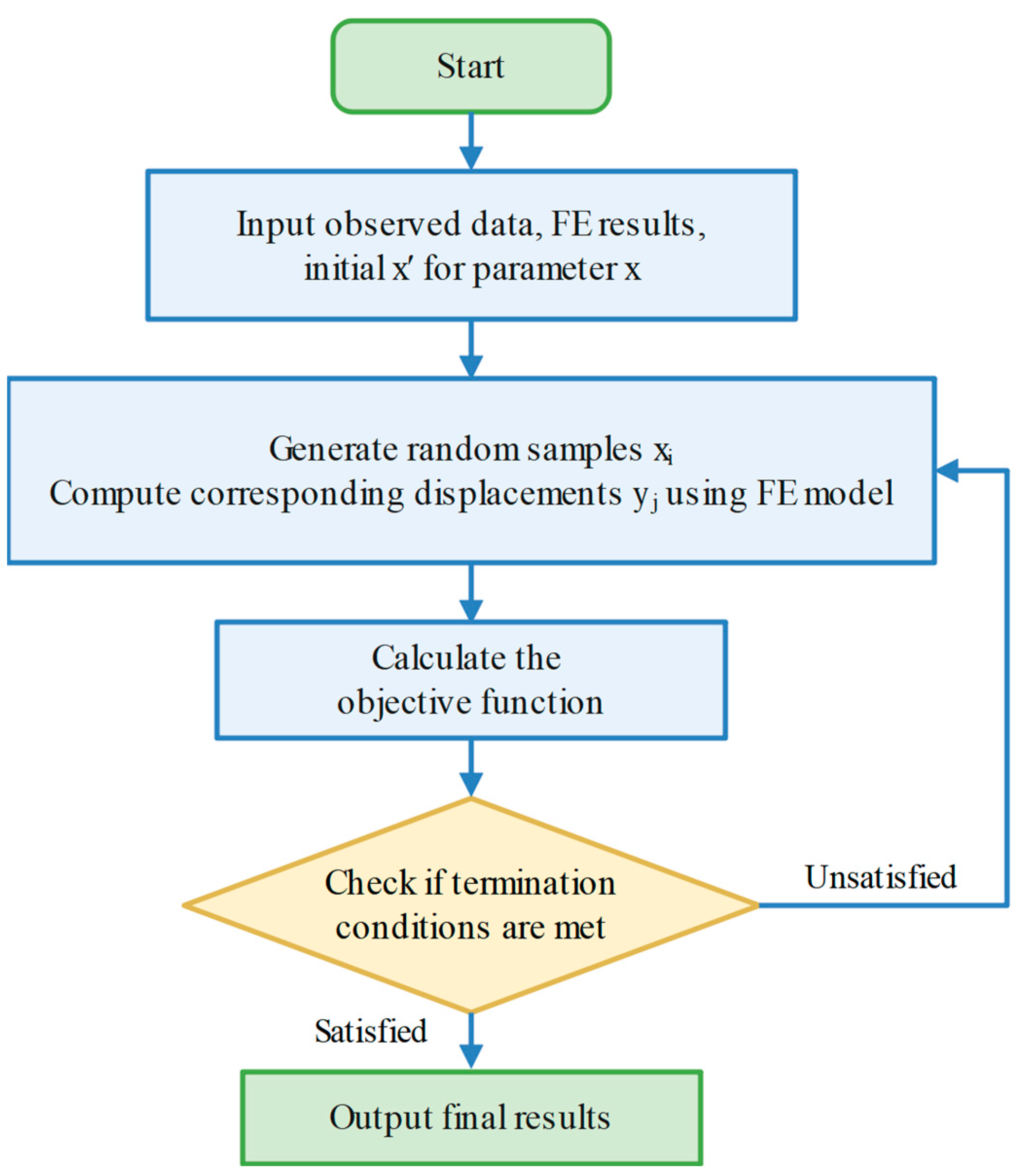
2. Inversion Methods for Mechanical Parameters of Concrete Gravity Dam

The estimation of mechanical parameters of dam concrete and bedrock usually relies on laboratory test data. However, such experimentally determined parameters often demonstrate significant discrepancies with in situ conditions due to scale effects and long-term environmental exposure. To address this limitation, inversion analysis methodology integrates numerical modeling with prototype monitoring data to accurately identify the time-dependent mechanical properties of dam–foundation systems [21,22].
The basic principles and methods for identifying the elastic modulus are as follows:
Divide the dam and dam base into two areas Ω 1 , Ω 2 .
Define the average elastic modulus and Poisson’s ratio of the materials in the two regions as E c , E r , μ r , μ c , respectively. In the elastic phase, the equilibrium equations of the whole structure are shown in Equation (1):
K δ H = R H
K is the overall strength matrix, which can be written as Equations (2) and (3):
K = e j Ω 1 C e j T K e j C e j + e j Ω 2 C e j T k e j C e j
k e j = Ω j B T D B d Ω = E Ω j B T f μ B d Ω = E k ¯ e j
where D = E f μ is the elasticity matrix; [ B ] is the cell geometry matrix; C e j is the strength transformation matrix of cell e j .
Since E = E c , e j Ω 1 E r , e j Ω 2 , Equation (2) can be written in the following form:
K = E c e j Ω 1 C e j T k ¯ e j C e j + R e j Ω 2 C e j T k ¯ e j C e j = E c f ( L , μ r , μ c , E r E c )
where R = E r E c ; L is the geometry of the dam.
If E r E c is certain, μ r and μ c are unchanged, then [ K ¯ ] = f ( L , μ r , μ c , E r E c ) . Equation (4) can be rewritten as Equation (5):
[ K ] = E c [ K ¯ ]
Simplification is given as Equation (6):
δ H = δ ¯ H / E c
where δ ¯ H = K ¯ 1 R H .
From Equation (6), the displacement of the dam body δ H induced by the reservoir water pressure is inversely proportional to E c when the ratio of the concrete and bedrock modulus of the dam body is a certain value under the reservoir water force.
The dam’s safety monitoring displacement is used as the target variable for inversion analysis. The objective function of the parameter inversion optimization problem is defined as the weighted sum of squares of the residuals between the finite element computed displacement and the measured displacement at the monitoring points. This approach aims to determine the basic parameter that most closely reflects actual conditions. The flowchart of the parameter inversion process is shown in Figure 1. This flowchart systematically outlines the iterative optimization framework, beginning with the initialization of observed data and finite element inputs, followed by stochastic parameter generation and displacement computation. The adaptive feedback loop, driven by the objective function evaluation and termination criteria, ensures continuous refinement of parameters until convergence. Notably, the integration of real-time monitoring data with numerical simulations highlights the algorithm’s capability to bridge empirical observations and theoretical models. While the flowchart provides a clear procedural structure, future enhancements could explicitly incorporate time-dependent parameter updating steps to better align with the dynamic inversion methodology proposed in this study.

3. Improved Particle Swarm Optimization Algorithm

3.1. Particle Swarm Algorithm Fundamentals

The particle swarm algorithm [23] is a global optimization evolutionary algorithm inspired by the collective behaviors of birds, such as feeding, migration, and flocking. It is known for its fast convergence and strong optimization capability. In this algorithm, the target solution of the optimization problem is abstracted as the feeding target of a bird flock, while potential solutions are represented as birds searching for food in a multidimensional space. To simplify the model, the flock is replaced with massless particles, each characterized by only two attributes: spatial position and evolutionary velocity [24].
In the search space, a particle’s position represents its current solution to the optimization problem. The algorithm evaluates each solution using a fitness function to determine its quality. Two key positions influence the optimization speed of each particle: the best solution found by an individual particle over time and the best solution found by any particle in the swarm. Through continuous iterations updating particle positions and velocities, the algorithm gradually converges to the optimal solution [25].
Individuals in the particle swarm (PSO) algorithm are called particles, and each swarm consists of N particles randomly initialized in a D dimensional search space. During the search process, each particle i is represented by two vectors, i.e., the velocity vector v i = v i 1 , v i 2 , , v i D and the position vector X i = x i 1 , x i 2 , , x i D . Each particle i updates its velocity and position using its personal historical best position P b e s t i =   p b e s t i 1 ,   p b e s t i 2 , ,   p b e s t i D , and the global best position found so far. For simplicity, P b i is used to refer to P b e s t i and P g is used to refer to G b e s t . The update formulas for v i and X i are shown in Equations (7) and (8):
V i d t + 1 = ω V i d t + c 1 r 1 P b i d t X i d t + c 2 r 2 P g d t X i d t
X i d t + 1 = X i d t + V i d t + 1
where V i d t and X i d t denote the velocity and position of the i particle at the t iteration in the d-th dimension; P b i d t is the best position searched by the i particle at the t iteration in the d-th dimension, and P g d t is the best position searched by the whole swarm at the t iteration. t and t + 1 are the current and next iterations, respectively. ω are the inertia weights, and c 1 and c 2 represent the acceleration coefficients of the particles with P b i d t and P g d t weights, respectively. r 1 and r 2 are random numbers in the range [0, 1]. The personal historical best position and global best position of each particle are updated in each iteration using Equations (9) and (10), respectively:
P b i d t + 1 = X i d t + 1 , f X i d t + 1 f P b i d t P b i d t , f X i d t + 1 > f P b i d t
P g d t + 1 = P g d t , f P g d t min i f P b i d t + 1 P b i d t + 1 , f P g d t > min i f P b i d t + 1
In the above equation, f is the objective function of the optimization problem, and P b i d and P g d are updated as an example for taking the minimum value. Thus, the particle velocity update equation (Equation (8)) consists of three components. The first is the inertia of the particle, which represents its tendency to maintain its previous velocity and is referred to as “memory”. The second component reflects the particle’s own knowledge, while the third accounts for information exchange and cooperation among particles, known as “socialization”. Although the standard particle swarm algorithm can be applied to robotic arm path planning, it has several limitations. For instance, a constant inertia weight is not conducive to balancing local and global searches. Additionally, as iterations progress, particles tend to converge to a local optimal solution, reducing population diversity and increasing the risk of the algorithm becoming trapped in a local optimum [26].

3.2. Improvement Strategy

The particle swarm optimization (PSO) algorithm differs from genetic algorithms in that it does not involve crossover or mutation operations. Instead, it relies solely on particle velocity to perform the search. During iterative evolution, only the information from the optimal particle is shared with other particles, resulting in a fast search speed. Additionally, PSO has a simple structure, requires fewer adjustable parameters, and is easy to implement in engineering applications. It employs real-number encoding, where the number of variables in the problem directly corresponds to the number of dimensions in the particle space, ensuring a direct representation of the optimization problem.
A key challenge in PSO is balancing global and local search capabilities, which remains a crucial issue in optimization [27]. To address this, an adaptive inertia weight parameter is introduced to enhance the algorithm’s performance. By adjusting inertia weights dynamically based on particle positions during the search process, the optimized PSO algorithm improves convergence toward the global optimum while reducing the risk of being trapped in a local optimum. The fundamental process of the algorithm is as follows.
Assuming that the number of kinetic–elastic modulus regions to be inverted is m and that an initial population is formed by n particles, the initial population of particles E in n × m space is Equation (11):
E = E 11 E 12 E 1 m E 21 E 22 E 2 m E n 1 E n 2 E n m
If the velocity v i = v i 1 , v i 2 , , v i m and position x i = x i 1 , x i 2 , , x i m of the first i particle in the population, after determining the initialized particle population information, the adaptation value J E i of each particle is calculated and the individual extreme value P i = P i 1 , P i 2 , , P i m and global extreme value g i = g i 1 , g i 2 , , g i m of the i-th particle in the population are determined at the same time. The particle determines the running direction and velocity of the next generation through its own experience and the experience of the group; for the k + 1 generation of particles, the velocity and position of the particle are updated as Equation (12) according to the following equation:
v i d k + 1 = ω v i d k + c 1 r 1 P i d k x i d k + c 2 r 2 g d k x i d k x i d k + 1 = v i d k + v i d k + 1 ω = ω min ω max ω min J t J min J a r g J min , J t J a r g ω max , J t > J a r g
where c 1 , c 2 is the learning factor; r 1 , r 2 are uniform random numbers in the range of [0, 1]; v i d k , x i d k are the velocity and position of the particle i in the d-th dimension of the k-th iteration; P i d k is the position of the particle i in the d-th dimension of the smallest individual adaptation value; g d k is the position of the particle in the d-th dimension of the smallest population adaptation value; ω is the inertia weights; ω min , ω max are the minimum and maximum of the inertia weights; J t represents the real-time adaptation value of the particle; J a r g , J min are the average and minimum fitness values, respectively, across all particles in the current iteration. When the number of iterations or the stop condition is reached, the search is stopped and the optimal value is output; otherwise, the search will continue to iterate and update the particles until the search reaches a value that satisfies the convergence criterion.

4. Engineering Examples

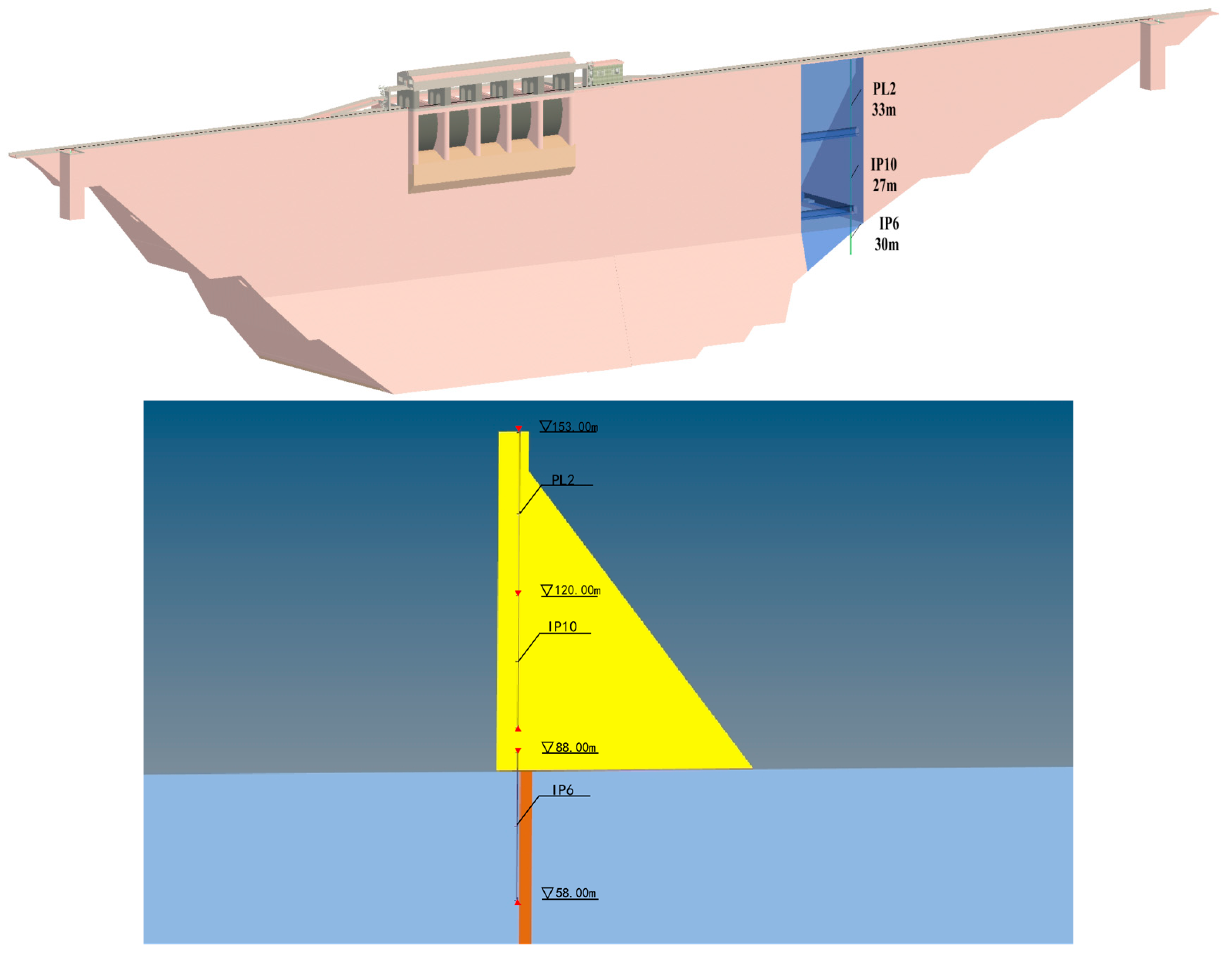
4.1. Overview of the Project

A hydropower dam pivot project is located in Cambodia. The main structure consists of a 112 m high roller-compacted concrete gravity dam, a five-gate spillway at the top of the dam, a PH3 diversion structure, a PH3 powerhouse, and a switching station. According to the 500-year flood design and the calibration of the Probable Maximum Flood (PMF), the reservoir’s key water levels are as follows: a calibration flood level of 151.88 m, a design flood level of 150.00 m, a normal storage level of 150.00 m, and a dead water level of 130.00 m. The reservoir has a total capacity of 717.3 million m3, with a dead water capacity of 354.2 million m3, and the capacity of the reservoir below the normal storage level of 681.3 million m3. The dam has a crest elevation of 153.00 m and a base elevation of 41.00 m, with a maximum height of 112.00 m. The dam crest is 6.0 m wide. The upstream face is vertical above 84 m, while below this elevation, it has a slope of 1:0.3. The downstream face has a slope of 1:0.75, with a slope break at 145.00 m.
To monitor horizontal displacement, a total of eight inverted plumb lines were installed at elevations of 153 m, 120 m, 88 m, 60 m, and 43 m on both the left and right banks of the dam. These instruments were designated as IP1–IP8, with displacement observations beginning on 21 March 2011. IP7 and IP8 were added in January 2014 and installed by July 2014, and their initial values were recorded. In 2018, additional plumb lines were installed in dam sections 4# and 7#, including IP9, PL1-1, PL1-2, and PL1-3 in section 4#, as well as IP10 and PL2 in section 7# (with IP6 as the reference point).
The dam foundation’s horizontal displacement is monitored using inverted plumb lines, which detect displacement in both the downstream and cross-river directions. The monitoring system consists of 10 inverted plumb line holes distributed across different elevations: IP7 in section 5 at the 43.00 m corridor, IP8 in section 6 at the 60.00 m corridor, IP5 and IP6 in sections 3 and 7 at the 88.00 m corridor, IP3 and IP4 in sections 2 and 9 at the 120.00 m corridor, and IP1 and IP2 at the 153.00 m elevation on the dam crest in sections 1 and 10.
Additionally, in 2018, new inverted plumb lines were added to sections 4# (IP9) and 7# (IP10). The monitoring layout is illustrated in Figure 2. The foundation’s inverted displacement was observed from baseline values recorded before reservoir impoundment. However, displacement data from the construction period are incomplete and not fully reflected. Since IP7 and IP8 were installed later as supplementary instruments, only post-2014 monitoring data are available. Initial values for IP9 and IP10 were recorded on 7 June 2018.
In this paper, the measured data of IP6, IP10, and PL2 installed at dam section 7 are used for inversion analysis. The dam section 7# is equipped with three plumb lines for monitoring the displacement in the upstream–downstream direction. A normal plumb line (PL2) was installed at a 153 m elevation. Two inverted plumb lines (IP10 and IP6) were installed at 120 m and 88 m elevations. The plumb line allows for measuring relative displacement between the two ends of the plumb line. For a normal plumb line, the upper end of the wire is fixed at the top of the dam, while a heavy weight is damped at its lower end. For an inverted plumb line, the plumb wire is fixed at the lower end, and the upper end of the wire is linked to a float submerged in a water box in the observation area. Observations are recorded digitally.

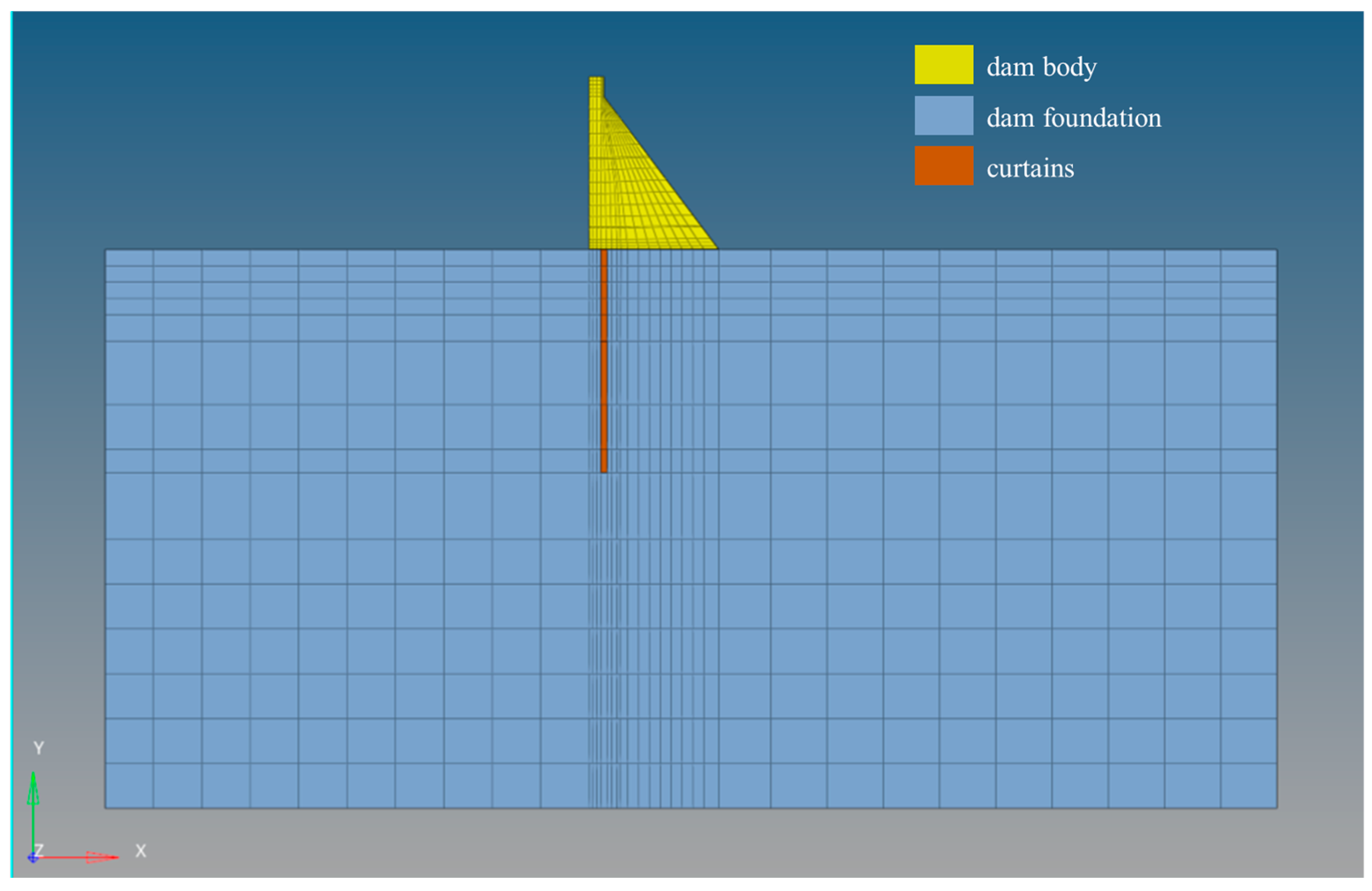
4.2. Finite Element Model and Calculation Parameters

In this study, the 7# section of the prototype dam was selected as the reference for the finite element numerical analysis. A two-dimensional finite element model was developed using HyperMesh for preprocessing and mesh generation. The finite element mesh includes 908 elements and 983 nodes. Based on the geometric and structural characteristics of the prototype and the arrangement of observation points, the FEM was established with the upstream dam foundation as the coordinate origin. The dam has a height of 69 m, and the foundation extends approximately twice the maximum dam height both upstream and downstream. Different structural regions were categorized and processed accordingly, dividing the model into three main components: the dam body, the dam foundation, and the curtain. The x-axis represents the downriver direction, while the y-axis corresponds to the vertical direction. The finite element discretization utilizes plane quadrilateral elements with four nodes. In the numerical simulation, normal displacement constraints are imposed on the peripheral boundaries of the foundation, while full fixity conditions are applied at the base. The external load includes the upstream water pressure. According to tests, the densities of the dam body and foundation are taken as 2.4 g/cm3 and 2.57 g/cm3, respectively. Moreover, it is already verified that the load–displacement response of the concrete dam is not highly influenced by the Poisson ratio; thus, the Poisson ratios of the dam body and foundation are taken as 0.167 and 0.25, respectively. The finite element model is illustrated in Figure 3.
The described FEM was implemented by GeHoMadrid, an FE program that was jointly developed between Technical University of Madrid (Spain) and Hohai University (China) [28]. The program was developed in Fortran and incorporates the PARDISO package for solving highly complicated and sparse equations. It is commonly used to solve complex structural, fluid, and multi-physics problems in geotechnical and hydraulic engineering.

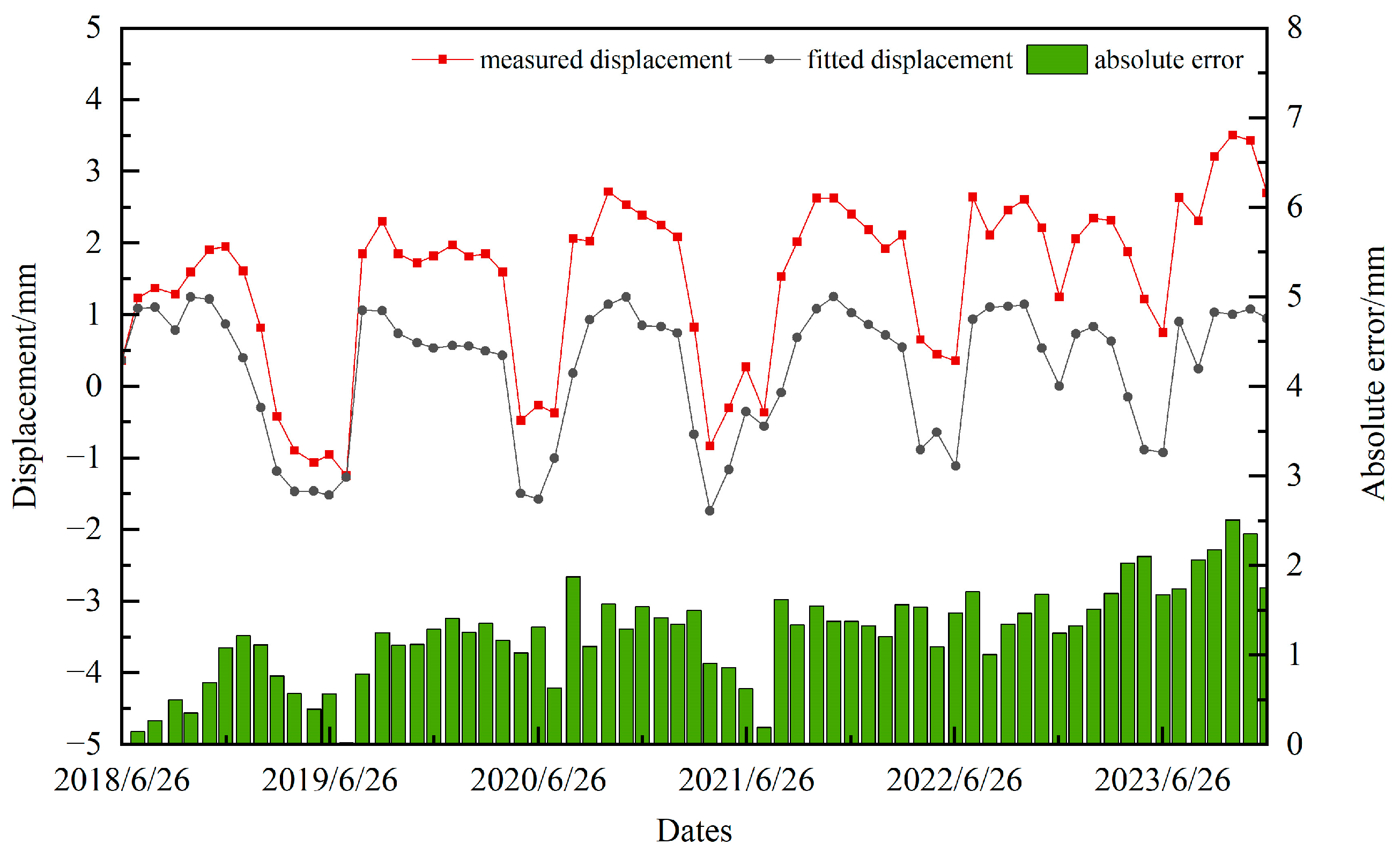
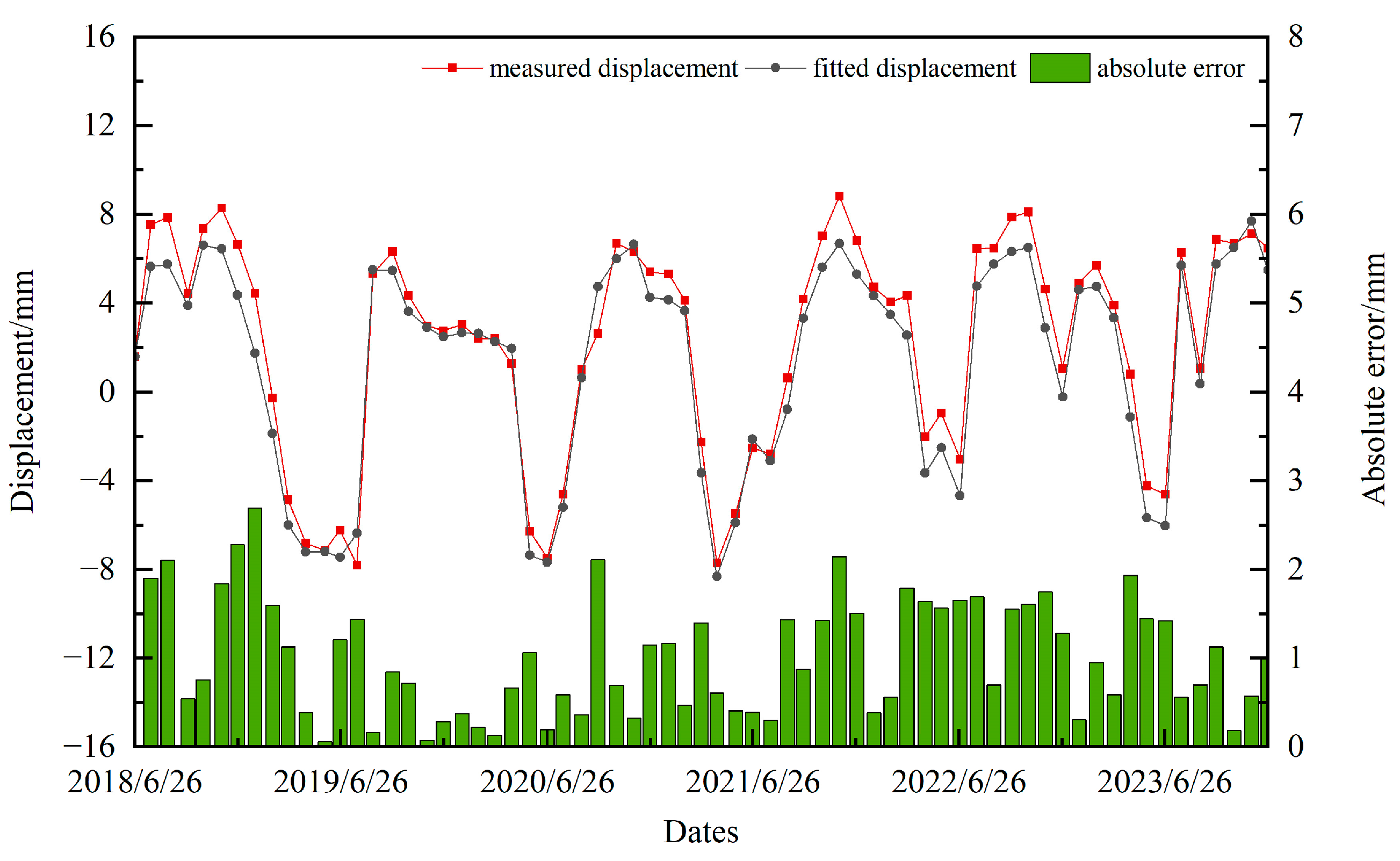
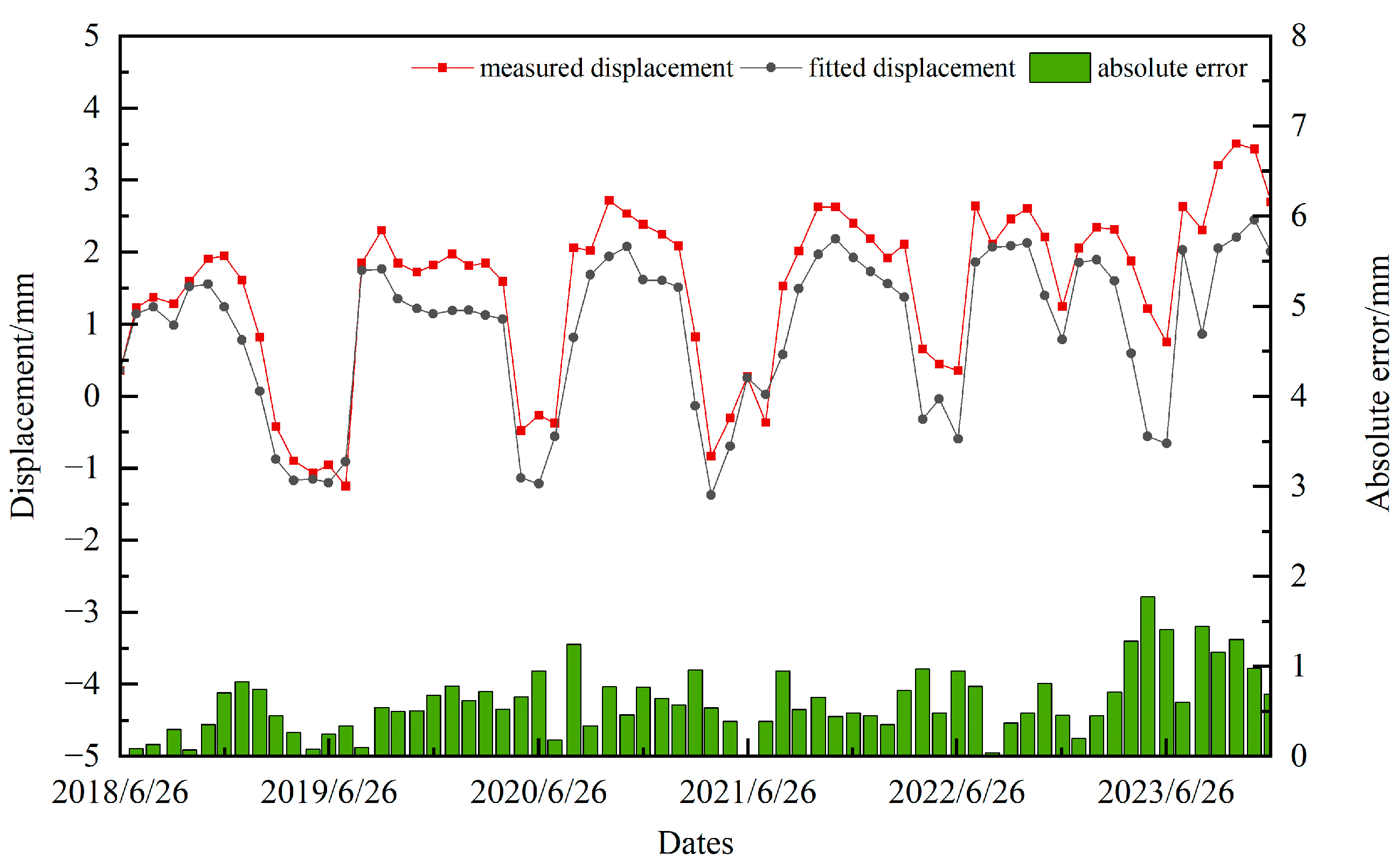
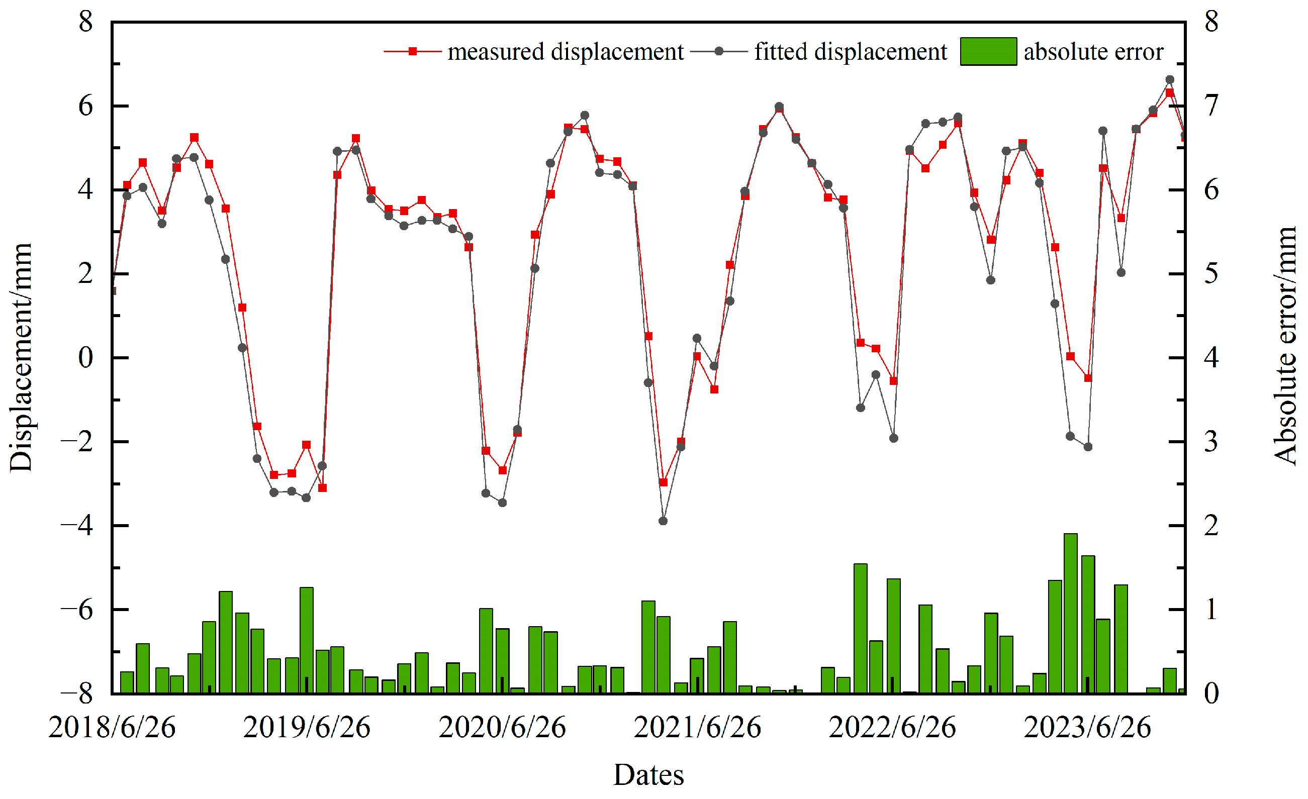
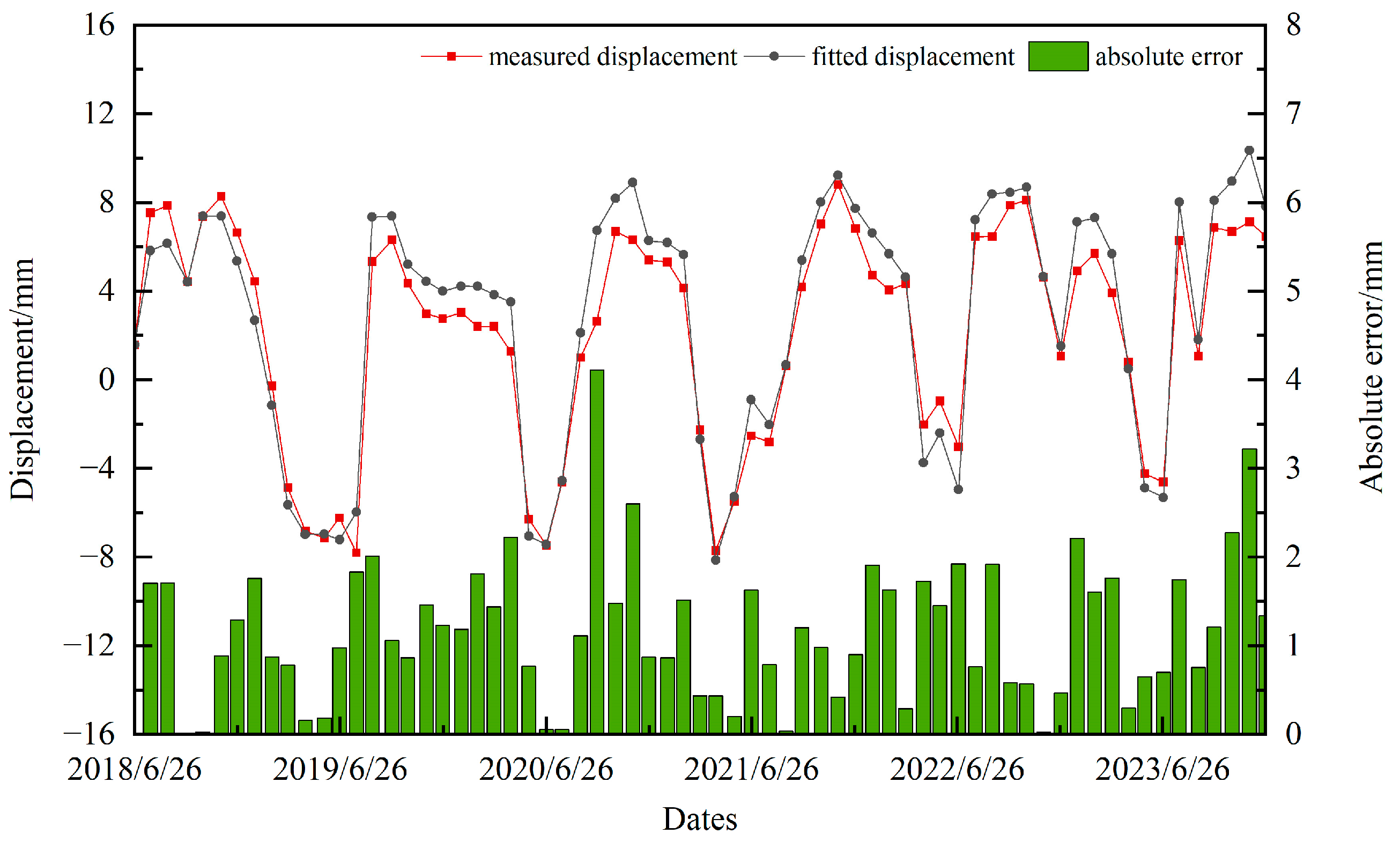
4.3. Comparison and Discussion

Dam section #7 is taken as a representative example in this study. The observed displacements of the plumb lines IP6, IP10, and PL2 in section #7 are shown in Figure 4, Figure 5 and Figure 6. Observations were recorded monthly from 26 June 2018 to 26 December 2023, for a total of 66 measurements. In the improved particle swarm algorithm, the population size is taken as 30; the maximum number of iterations is 30; the inertia weight maximum and minimum values are taken as ω max = 0.8, ω min = 0.2; the learning factor c 1 = c 2 = 1.5, e 1 = 0.8, e 2 = 0.4. According to the preliminary calculations, the ranges of values of the mechanical parameters are set as E 17   GPa , 25   GPa for the dam body and E 2   GPa , 6   GPa for the dam foundation. The inversion results are 20.74 GPa for the dam body and 4.67 GPa for the dam foundation. The fitted displacements based on the calibration numerical model are shown in Figure 4, Figure 5 and Figure 6.
The general consistency between measured and inverted displacement trends across most monitoring points can be observed from the figures. However, a larger discrepancy is noted at measurement points especially near the dam foundation.
Based on the fitted results of the static parameter inversion, it is initially inferred that parameter weakening occurs in the dam foundation, while the dam body remains in an elastic working condition. Therefore, the elastic modulus of the dam body is determined to be 20.74 GPa based on the static inversion results. The dynamic inversion analysis incorporated field data from three positioned monitoring points (IP6, IP10, and PL2) in dam section 7#. The calculation results reveal a clear temporal degradation pattern in the mechanical properties of the dam foundation, which was quantitatively characterized through curve fitting. Figure 7 presents the time-dependent reduction in the elastic modulus of the dam foundation.
The time-varying functions of material parameters, such as those of geotechnical bodies and concrete, are typically modeled using exponential or logarithmic functions [29,30]. The time-dependent reduction in the elastic modulus of the dam foundation is fitted as the equation y = 1.075 e ^ ( 0.114 x ) + 3.829 . The time-dependent elastic moduli obtained from the dynamic inversion analysis are sequentially implemented in the finite element program to compute theoretical displacements. The fitted displacements compared against field measurements are shown in Figure 8, Figure 9 and Figure 10.
The measured and simulated displacement time series exhibit strong agreement across all monitoring points (Figure 8, Figure 9 and Figure 10), demonstrating the effectiveness of the dynamic inversion analysis. In addition, two statistical metrics, the Mean Absolute Error (MAE) and Root Mean Square Error (RMSE), are employed to quantitatively evaluate the model performance, as defined in Equations (13) and (14):
R M S E = 1 N i = 1 N x ^ i x i 2
M A E = 1 N i = 1 N x ^ i x i
where N is the number of sequences; x ^ i and x i are the fitted and measured values of the displacement, respectively.
The results are shown in Table 1 and Table 2.
The calculation results indicate that the fitting accuracy of the measurement points at the dam foundation is significantly improved in the dynamic inversion model compared to the static inversion model. Although the errors of measurement points at the dam body are slightly larger than those of the static inversion model, the overall prediction errors remain lower than those of the static inversion model. The primary sources of error can be attributed to two factors. First, the observed data contain random errors due to limitations in measurement instrument accuracy and environmental influences. Second, the numerical model itself introduces inherent errors arising from simplified assumptions and uncertainties in mechanical parameters. This suggests that parameter weakening occurs at the dam foundation and that the weakening trend gradually stabilizes. These results demonstrate time-dependent stiffness degradation in the dam foundation, with the rate of modulus reduction decreasing asymptotically over time.

5. Conclusions

This study presents a comprehensive investigation into the long-term deformation behavior of concrete gravity dams on soft rock foundations, with a focus on dynamic parameter inversion using an improved particle swarm optimization (PSO) algorithm. The conclusions are as follows:
(1) The inversion analysis successfully quantified the elastic moduli of the dam body and foundation, while capturing the time-dependent degradation of the foundation’s elastic modulus through an exponential decay model. The identified mechanical parameters provide a critical baseline for evaluating the structural performance and long-term safety of the dam.
(2) The improved PSO algorithm, incorporating adaptive inertia weight, achieves robust global optimization with stable convergence. Integrated with finite element modeling and real-time monitoring data, the inversion framework enables high-precision displacement predictions of the concrete dam.
(3) The proposed dynamic inversion method has exhibited significant effectiveness in assessing the long-term performance of the concrete gravity dam constructed on a soft rock foundation. To further advance the research, Bayesian updating theory will be introduced to systematically quantify the uncertainties in both monitoring data and numerical models, with the ultimate objective of establishing reliable risk warning indicators.

Author Contributions

Methodology, T.L.; Software, C.L. and T.L.; Validation, T.S. and W.X.; Data curation, G.Y.; Writing—original draft, G.Y. and C.L.; Writing—review and editing, W.X. and S.C.; Project administration, C.L. All authors have read and agreed to the published version of the manuscript.

Funding

This research was funded by the National Key Research and Development Program of China (No. 2022YFC3005403), the National Natural Science Foundation of China (Nos. 52309151 and 52309157), the Open Research Fund of Key Laboratory of Reservoir and Dam Safety Ministry of Water Resources (No. YK323007), and the Science and Technology Project of Power Construction Corporation of China (No. DJ-HXGG-2022-02).

Data Availability Statement

The data presented in this study are available on request from the corresponding author.

Conflicts of Interest

Author Guanglin Yin was employed by the company Nanjing Hohai NARI Hydroelectric Automation Co., Ltd. The remaining authors declare that the research was conducted in the absence of any commercial or financial relationships that could be construed as a potential conflict of interest.

References

  1. Chen, S.; Lin, C.; Gu, Y.; Sheng, J.; Hariri-Ardebili, M.A. Dam Deformation Data Preprocessing with Optimized Variational Mode Decomposition and Kernel Density Estimation. Remote Sens. 2025, 17, 718. [Google Scholar] [CrossRef]
  2. Xiang, Y.; Su, H.; Wu, Z. Inversion of Physico-Mechanical Parameters Based on Dam Safety Monitoring Data. J. Water Resour. 2004, 35, 98–102. [Google Scholar] [CrossRef]
  3. Lin, C.; Chen, S.; Hariri-Ardebili, M.A.; Li, T. An Explainable Probabilistic Model for Health Monitoring of Concrete Dam via Optimized Sparse Bayesian Learning and Sensitivity Analysis. Struct. Control Health Monit. 2023, 2023, 2979822. [Google Scholar] [CrossRef]
  4. Huang, Y.; Huang, G.; Wu, Z.; Shen, Z. Optimized Inversion of Time-Varying Parameters of Concrete Dams Based on Deformation Monitoring Data. J. Rock Mech. Eng. 2007, 26, 2941–2945. [Google Scholar]
  5. Lin, C.; Li, T.; Chen, S.; Yuan, L.; van Gelder, P.; Yorke-Smith, N. Long-term viscoelastic deformation monitoring of a concrete dam: A multi-output surrogate model approach for parameter identification. Eng. Struct. 2022, 266, 114553. [Google Scholar] [CrossRef]
  6. Lin, C.; Du, X.; Chen, S.; Li, T.; Zhou, X.; van Gelder, P.H.A.J.M. On the multi-parameters identification of concrete dams: A novel stochastic inverse approach. Int. J. Numer. Anal. Methods Geomech. 2024, 48, 3792–3810. [Google Scholar] [CrossRef]
  7. Wang, P.; Zhu, W.; Wang, K. Simplex Shape Method and Its Application to Inversion analysis of Perimeter Rock Deformation in Guangzhu Power Station. Geotech. Mech. 1991, 12, 57–66. [Google Scholar]
  8. Wu, X.; Wu, Z.; Gu, C.; Shen, Z.; Shu, Y. Inversion analysis Method of Creep of Crushed Concrete Arch Dam. Dam Obs. Civ. Test. 2000, 24, 22–24, 35. [Google Scholar]
  9. Niu, J. Inversion analysis of Mechanical Parameters of Crushed Concrete Dam Based on Chaotic Genetic Algorithm. South-to-North Water Divers. Water Sci. Technol. 2012, 10, 140–143. [Google Scholar]
  10. Wan, Z.; Huang, Y.; Zhu, Z.; Wang, T.; Jing, J.; Xiao, L. Inversion Analysis of Mechanical Parameters During Operation Period of Crushed Concrete Dam in Alpine Area. Water Conserv. Hydropower Technol. 2017, 48, 50–55. [Google Scholar]
  11. Li, W.; Liu, Q.; Shi, E.; Guo, W. Parameter Inversion and Application of South Water Modeling for Rockfill Based on XGBoost Algorithm. J. Water Resour. Water Transp. Eng. 2023, 111–120. [Google Scholar] [CrossRef]
  12. Sun, T.; Chen, Y.; Chen, J.; Yang, B.; Tan, C. Stability Modeling of Typical Dam Foundation of Daitengxia Lock and Dam. J. Undergr. Space Eng. 2022, 18, 179–189. [Google Scholar]
  13. Tang, M.; Duan, B.; Zhang, L.; Chen, J.; Yang, B. Experimental Study on Geomechanical Modeling of Overall Stability of High Gate Dam on Deep and Thick Overburden. Hydropower Gener 2017, 43, 105–109. [Google Scholar]
  14. Tian, Y.; Chen, W.; Tian, H.; Zhao, M.; Zeng, C. Study on the Design of Buffer Layer Letting Pressure Support Considering the Time-Dependent Weakening of Soft Rock Strength. Geotech 2020, 41 (Suppl. S1), 237–245. [Google Scholar]
  15. Li, S.; Wei, L.; Niu, J.; Deng, Z.; Wu, B.; Qian, W.; He, F. Time-Dependent Deviation of Bridge Pile Foundations Caused by Adjacent Large-Area Surcharge Loads in Soft Soils and Its Preventive Measures. Front. Struct. Civ. Eng. 2024, 18, 184–201. [Google Scholar] [CrossRef]
  16. Liu, B.; Li, H.; Wang, G.; Huang, W.; Wu, P.; Li, Y. Dynamic Material Parameter Inversion of High Arch Dam under Discharge Excitation Based on the Modal Parameters and Bayesian Optimised Deep Learning. Adv. Eng. Inform. 2023, 56, 102016. [Google Scholar] [CrossRef]
  17. Tian, K.; Yang, J.; Cheng, L. Deep Learning Model for the Deformation Prediction of Concrete Dams under Multistep and Multifeature Inputs Based on an Improved Autoformer. Eng. Appl. Artif. Intell. 2024, 137, 109109. [Google Scholar] [CrossRef]
  18. Yan, S.; Jiayuan, F.; Chuan, L. Prediction Model of Dam Structure Dynamic Deformation Based on Time Attention Mechanism. J. Hydroelectr. Eng. 2022, 41, 72–84. [Google Scholar]
  19. Liu, C.; Pan, J.; Wang, J. An LSTM-Based Anomaly Detection Model for the Deformation of Concrete Dams. Struct. Health Monit. 2023, 23, 1914–1925. [Google Scholar] [CrossRef]
  20. Madiniyeti, J.; Chao, Y.; Li, T.; Qi, H.; Wang, F. Concrete Dam Deformation Prediction Model Research Based on SSA–LSTM. Appl. Sci. 2023, 13, 7375. [Google Scholar] [CrossRef]
  21. Su, H.; Li, J.; Wu, Z. Optimization of inversion analysis of dam and foundation physico-mechanical parameters. J. Water Resour. 2007, S1, 129–134. [Google Scholar]
  22. Lin, C.; Li, T.; Chen, S.; Lin, C.; Liu, X.; Gao, L.; Sheng, T. Structural identification in long-term deformation characteristic of dam foundation using meta-heuristic optimization techniques. Adv. Eng. Softw. 2020, 148, 102870. [Google Scholar] [CrossRef]
  23. Kennedy, J.; Eberhart, R. Particle Swarm Optimization. In Proceedings of the ICNN’95-International Conference on Neural Networks, Perth, WA, Australia, 27 November–1 December 1995; IEEE: Piscataway, NJ, USA, 1995; Volume 4, pp. 1942–1948. [Google Scholar]
  24. Ocampo, E.; Liu, C.-H.; Kuo, C.-C. Performance Analysis of Partitioned Step Particle Swarm Optimization in Function Evaluation. Appl. Sci. 2021, 11, 2670. [Google Scholar] [CrossRef]
  25. Wang, D.; Tan, D.; Liu, L. Particle Swarm Optimization Algorithm: An Overview. Soft Comput. 2018, 22, 387–408. [Google Scholar] [CrossRef]
  26. Rini, D.P.; Shamsuddin, S.M.; Yuhaniz, S.S. Particle Swarm Optimization: Technique, System and Challenges. Int. J. Comput. Appl. 2011, 14, 19–26. [Google Scholar] [CrossRef]
  27. Shi, Y.; Eberhart, R. A Modified Particle Swarm Optimizer. In Proceedings of the IEEE International Conference on Evolutionary Computation Conference, Anchorage, AK, USA, 4–9 May 1998; pp. 69–73. [Google Scholar]
  28. Fernandez-Merodo, J.A.; Castellanza, R.; Mabssout, M.; Pastor, M.; Parma, M. Coupling transport of chemical species and damage of bonded geomaterials. Comput. Geotech. 2007, 34, 200–215. [Google Scholar] [CrossRef]
  29. Cheng, X. Time-Varying Reliability Analysis Model and Reliability Calculation Method for Rocky Slope Anchoring Project. Ph.D. Thesis, Hunan University, Changsha, China, 2010. [Google Scholar]
  30. Peng, H.; Liu, D.; Tian, B. Time-Varying Modeling of Safety and Reliability of Concrete Gravity Dams. Hydropower Gener. 2009, 35, 77–79. [Google Scholar]
Figure 1. Flowchart of inversion analysis.
Applsci 15 04750 g001
Figure 2. Arrangement of deformation monitoring of section 7# of a gravity dam.
Applsci 15 04750 g002
Figure 3. Two-dimensional finite element model of dam section 7#.
Applsci 15 04750 g003
Figure 4. The measured and fitted displacements of IP6 (static inversion analysis).
Applsci 15 04750 g004
Figure 5. The measured and fitted displacements of IP10 (static inversion analysis).
Applsci 15 04750 g005
Figure 6. The measured and fitted displacements of PL2 (static inversion analysis).
Applsci 15 04750 g006
Figure 7. The time-dependent reduction in the elastic modulus of the dam foundation (2018–2023).
Applsci 15 04750 g007
Figure 8. The measured and fitted displacements of IP6 (dynamic inversion analysis).
Applsci 15 04750 g008
Figure 9. The measured and fitted displacements of IP10 (dynamic inversion analysis).
Applsci 15 04750 g009
Figure 10. The measured and fitted displacements of PL2 (dynamic inversion analysis).
Applsci 15 04750 g010
Table 1. The evaluation results of the static inverse analysis.
Evaluation Indicators IP6IP10PL2
RMSE/mm1.3440.6141.193
MAE/mm1.2300.5211.000
Table 2. The evaluation results of the dynamic inversion analysis.
Evaluation Indicators IP6IP10PL2
RMSE/mm0.7070.7011.401
MAE/mm0.6040.5301.150
Disclaimer/Publisher’s Note: The statements, opinions and data contained in all publications are solely those of the individual author(s) and contributor(s) and not of MDPI and/or the editor(s). MDPI and/or the editor(s) disclaim responsibility for any injury to people or property resulting from any ideas, methods, instructions or products referred to in the content.

