Interpretable Machine Learning for Population Spatialization and Optimal Grid Scale Selection in Shanghai

Abstract

Fine-scale population distribution information is crucial for applications in urban public safety, planning, and management. However, when using machine learning methods for population spatialization, issues such as data overfitting and limited interpretability need to be addressed. This study introduced a combined approach using eXtreme Gradient Boosting (XGBoost) and SHapley Additive exPlanation (SHAP) to estimate population spatialization at various grid scales and interpret the key influencing factors, then we applied accuracy evaluation metrics and landscape ecology indices to identify the optimal grid scale. The results showed that the XGBoost model outperformed the WorldPop dataset in accuracy across all grid scales, with determination coefficients (R²) consistently exceeding 0.83. The SHAP analysis revealed that the primary influencing factors were the address, access, and dwelling characteristics of points of interest (POIs). The influence of these factors showed regional variations, with urban centers having a strong positive effect, while the negative influence increased with the distance to suburban areas. The population density estimates across different grid scales consistently exhibited a spatial gradient pattern of decreasing density from the urban center toward suburban areas. Based on comprehensive evaluations of accuracy and spatial heterogeneity, the 100 m grid was identified as the optimal scale for Shanghai’s population spatialization. The proposed XGBoost-SHAP population spatialization method demonstrates high reliability and generalizability, effectively explaining the heterogeneity of population distribution. This approach not only provides critical decision-making support for urban planning but also serves as a methodological reference for high-resolution population spatialization studies in other cities.

1. Introduction

China’s rapid urbanization has triggered massive rural-to-urban migration, creating significant governance challenges, particularly in megacities. Consequently, acquiring high-resolution spatial population distribution data has become crucial for urban planning, emergency management, public service provision, and economic development [1,2]. Traditional population distribution data are typically collected based on administrative divisions through surveys and statistical methods. However, this approach requires significant human and material resources, involves lengthy cycles, and suffers from coarse spatial granularity. As a result, it struggles to capture the spatial heterogeneity of population distribution within administrative regions and fails to accurately reflect population distribution patterns [3,4]. To address these limitations, scholars have explored various population spatialization estimation methods to improve both the accuracy and spatial resolution of population estimates [5].

The development of models and methods is central to research on urban population spatialization. In the early stages, various methods were used for population spatialization, including population density models, spatial interpolation methods, and statistical regression methods [6]. Population density models, including the Clark model, normal density model, Smeed model, and Gamma model [4,7,8,9], are grounded in urban geography theory and describe the decline in population density from the city center to the periphery. However, their estimation accuracy and spatial scale often fall short of contemporary demands for refined population management. Spatial interpolation methods, which assume that adjacent locations share similar characteristics, convert regional demographic data from a source spatial scale to a target scale, typically using downscaling techniques like point interpolation and area interpolation [10]. While these methods enable scale conversion, they often neglect boundary effects and fail to incorporate multiple factors influencing population distribution, leading to inaccurate population estimates in heterogeneous regions [11,12]. Statistical regression methods, such as geographically weighted regressions [13], multiple linear regressions [14], and support vector regressions [15], construct quantitative models of population spatial distribution using multi-source geographic data. Although these methods can capture the complex relationships between various factors and population spatial distribution, they struggle to reveal nonlinear relationships. Additionally, it is difficult to integrate multi-source heterogeneous data in the modeling process [16].

With the development and application of technologies such as geographic information systems, remote sensing, and big data, numerous new data sources have emerged. These sources, including nighttime light data, social network data, and mobile phone data, provide rich contextual information, detailed attributes, and a fine spatial resolution. The effective integration and utilization of multi-source data provide a new paradigm for population spatialization methods [17,18]. Among these approaches, machine learning has become increasingly prominent and is now the dominant methodology. Models such as random forest [19] and XGBoost [20] have been widely adopted. Wang [21] and He [22] constructed a random forest model based on multi-source data to achieve population spatialization in Tibet and Beijing. Zhao et al. [23] employed an XGBoost model to estimate population distribution at a 100 m grid scale in Shenzhen. Both models are based on decision tree algorithms. The random forest model demonstrates strong noise resistance and can effectively simulate complex nonlinear relationships between population distribution and influencing factors through factor weighting. However, its predictive capability is limited to the range of the training dataset in regression problems, which can lead to data overfitting. In contrast, the XGBoost model can quickly process multiple types of input data, incorporate built-in cross-validation and tree pruning, and offer greater flexibility in controlling data overfitting compared to other models [24].

Population spatial distribution is influenced by multiple factors, and understanding the degree and spatial characteristics of these influences is critical for developing high-quality urban planning and population spatialization policies. Machine learning models are often regarded as ‘black box’ methods because they typically do not explicitly reveal the relative importance of the key factors driving change. While models such as random forest and XGBoost can output the relative importance of various factors, they cannot effectively reveal the spatial extent of these influences. The SHAP interpretability method addresses this limitation by combining the robust data-fitting abilities of machine learning with a clear interface for the quantitative interpretation of results [25,26]. With the wide application of machine learning coupled with SHAP, this method has been gradually applied to quantify the contributions of influencing factors. For instance, Liu et al. [27] employed interpretable machine learning to explore the contributions of temperature, precipitation, soil moisture, and land use to vegetation changes in the Yellow River Basin. Similarly, Li et al. [28] integrated XGBoost with SHAP to analyze the impact of climatic factors on the long-term average net primary productivity (NPP) of the Amazon rainforest. The SHAP interpretability method not only ranks the importance of influencing factors but also effectively reveals their spatial distribution and degree of influence [29,30]. This capability provides valuable methodological support for interpreting the factors that influence urban population spatial distribution.

Significant progress has been made in population spatialization research. However, in the era of big data, the challenge of selecting appropriate estimation models to efficiently generate high-precision population spatial distribution data and interpret influencing factors remains. Additionally, many current studies rely on empirical approaches to determine optimal grid sizes for population estimation. As grid size significantly impacts the accuracy of fine-scale population and socioeconomic distribution data [31], determining the optimal spatial unit remains a critical research gap in refined population spatialization studies. Shanghai, a typical megacity in China, is characterized by a high population density, high degree of mobility, and uneven spatial distribution, making its population distribution more complex compared to smaller cities. The “Shanghai Urban Master Plan (2017–2035)” emphasized the need to optimize population layout, adjust population density, and promote the development of a livable city. These policy goals underscore the practical importance of conducting refined spatial population studies in Shanghai, which would enhance urban management and support sustainable development.

To address the critical challenges of machine learning overfitting in population spatialization, the difficulty in analyzing the spatial heterogeneity of key influencing factors, and the selection of optimal grid scales, this study takes Shanghai as a case study to develop a refined multi-scale modeling framework. Building upon a comprehensive multi-dimensional feature database, we construct an XGBoost-based population spatialization model integrated with SHAP (SHapley Additive exPlanations) interpretability methods. Our approach achieves three key objectives: (1) generating multi-scale population distribution maps for Shanghai, (2) quantifying and spatially characterizing the influence of key determinants, and (3) identifying the optimal grid resolution. The results provide both technical support for Shanghai’s population monitoring and a transferable methodology for other cities’ high-resolution population spatialization research.

2. Materials and Methods

2.1. Data Sources and Preparation

Population spatial distribution is influenced by a variety of cultural and natural factors. Therefore, this study employs multiple geospatial datasets for population spatialization modeling, including Luojia-1 (LJ1-01) nighttime light data, water area data, land use data, DEM data, and POI data. The model’s estimation accuracy is verified using 2018 statistical data from street (town) administrative units, as well as the WorldPop dataset. The main data sources are shown in

Table 1. Data sources.

Name	Data Sources
POI	AutoNavi Map Open Platform (https://lbs.amap.com/)
Luojia-1 Remote Sensing Image	High Resolution Earth Observation System Hubei Data and Application Center (http://59.175.109.173:8888/)
Administrative Division Data	Resource and Environmental Science Data Center (http://www.resdc.cn/)
Street (Town) Population Data	2019 Statistical Yearbook of Shanghai Districts
WorldPop Dataset	Institute for Geographic Data, University of Southampton, UK (http://www.worldpop.org/)
DEM	Geospatial Data Cloud (http://www.gscloud.cn/)
Land Use Data	Shanghai Land Use Status Database in 2017
OSM Water Area Data	OpenStreetMap (https://www.openstreetmap.org/)

.

POI data were obtained from the AutoNavi Map Open Platform in Shanghai using Python. To address the excessive variety in raw POI data and the limited representation of certain POI types, we conducted systematic data processing, including screening, removal, reclassification, and consolidation according to China’s national standard GB/T 35648-2017 [32] for classification and coding of geographic information points of interest. This procedure resulted in 17 dominant POI categories, each constituting more than 0.5% of the total dataset, ultimately yielding over 800,000 pieces of information. These categories included catering services, scenic spots, public facilities, enterprises, shop services, traffic services, address information, financial services, transportation facilities, education and cultural services, life services, dwellings, access facilities, relaxation services, hospital services, government agencies, social organizations, and hostel services. Using the geographical coordinates from the POI data, the tabular data was converted into vector point files, yielding a total of 1,236,242 POI data points. Building upon this framework, we performed localized kernel density estimation (KDE) for each individual POI category as well as their aggregated totality using the Silverman kernel function with a 400 m search radius (equivalent to 4 grid cells). The analysis produced density raster maps (units: features/km²) for each POI type, which were then spatially joined to 100 m × 100 m grid cells using GIS spatial linkage tools. This process ultimately generated an 18-dimensional feature set comprising both individual POI category densities and their combined total density values.

The 2018 nighttime light data for Shanghai, captured by the LJ-01 satellite, were obtained through downloading, stitching, and cropping. The data had an image digital number (DN) value range from 0 to 1,087,800 and a spatial resolution of 130 m. To ensure consistency with other datasets, the nighttime light data were resampled to 100 m resolution, transformed from the original CGCS2000 coordinate system to WGS-84, and radiometrically calibrated using the official formula provided by the data source website. The DN values, radiant brightness values, and binary processing results for light brightness were extracted to derive the three-dimensional features of the nighttime light data, which were then incorporated into the 100 m geographic grid.

$$L=D{N}^{{\displaystyle \frac{3}{2}}}\times {10}^{-10}$$

(1)

where L represents the radiance value after absolute radiometric correction, while DN denotes the grayscale value of LJ-01 nighttime light data.

The DEM data were also referenced to the WGS 84 coordinate system, with a spatial resolution of 30 m, which was resampled to 100 m for consistency. Using Shanghai’s administrative boundaries, the DEM image was stitched and cropped to extract the relevant elevation data. From this processed DEM, four dimensional features were derived: altitude, slope, aspect, and terrain undulation, and their corresponding values were then extracted and integrated into the 100 m geographic grid.

According to the “Technical Specifications and Preparation Guidelines for the Master Plan for Economic and Social Development of Cities and Counties (for Trial Implementation)”, jointly issued by the State Bureau of Surveying and Mapping and the National Development and Reform Commission of the People’s Republic of China in 2015, territorial space is categorized into three types: urban space, agricultural space, and ecological space. By integrating these guidelines with the “Current Land Use Classification Standard” (GB/T21010-2017) [33], Shanghai’s 2018 land use data were categorized into urban land space, agricultural land space, and ecological land space, thereby deriving three-dimensional land use features.

The water area data were obtained from a dataset downloaded from the OSM official website. In accordance with the principle of “no land, no population”, all water areas were assigned a population value of 0. Additional features incorporated into the dataset included grid ID, district/county names, and street names. All derived features were then integrated into the geographic grid to establish a 28-dimensional population spatialization feature database for Shanghai. It should be noted that this study employs 2018 township-level population statistics, Luojia-1 nighttime light data (2018), 2020 POI data, and land use data from late 2017. While the temporal discrepancies may have some degree of influence on the results, the overall time differences remain within acceptable limits. All feature data were resampled to the required grid scales using ArcGIS software.

2.2. Methods

2.2.1. XGBoost Model

XGBoost is an efficient machine learning model with strong generalization ability, developed by Chen and Guests based on the Gradient Boosting Decision Tree (GBDT) algorithm. The model incorporates key innovations including regularization terms and parallel computing techniques [34]. It operates by iteratively learning multiple decision functions through an ensemble of decision trees, in which each subsequent tree corrects errors from previous predictions. The final prediction is obtained by aggregating weighted outputs from all trees in the ensemble. The regression tree function used in XGBoost can be expressed as follows:

$${\widehat{y}}_i=\phi ({{\rm X}}_i)={\displaystyle \sum _{k=1}^K{f}_k}({{\rm X}}_i),f_k\in F$$

(2)

where $f(x)$ represents a regression tree function; ${\stackrel{\wedge }{y}}_i$ is the predicted value of the model; K is the number of decision trees; $f_k$ represents the $k^{th}$ sub-model; $X_i$ represents the $i^{th}$ input sample; $F=\left\{f(x)={\omega }_{q(x)}\right\}(q:R^m\to T,\omega \in R^T)$ indicates the space of the regression tree; and ${\omega }_{q(x)}$ represents the fraction of leaf nodes q. Based on the predicted values of the regression tree described above, an objective function of the model is available:

$$O_{\mathrm{bj}}={\displaystyle \sum _{i=1}^{n}l(y_i,{\widehat{y}}_i)+{\displaystyle \sum _{k=1}^K\Omega (f_k)}}$$

(3)

where $n$ is the total amount of data imported for the $k^{th}$ regression tree; K represents all regression trees built; ${\displaystyle \sum _{\mathrm{i}=1}^{n}l(y_i,{\widehat{y}}_i)}$ represents the loss function of the objective function; and ${\displaystyle \sum _{k=1}^K\Omega (f_k)}$ represents the regularization term of the objective function. The specific functions are as follows:

$$\Omega (f_k)=\gamma T+{\displaystyle \frac{1}{2}}\lambda {‖\omega ‖}^2$$

(4)

where $T$ represents the number of leaf nodes of the regression tree; $\omega$ represents the fraction of the leaf node of the regression tree; and $\gamma ,\lambda$ represents the penalty coefficient of the regular term. The optimal value of the loss function in the $t^{th}$ iteration when the structure of the tree is fixed is as follows:

$$w_j^{\ast }={\displaystyle \sum _{i\in I_J}\frac{g_i}{h_i+\lambda }}$$

(5)

According to the principle of XGBoost algorithm, the residues of the previous prediction need to be fitted into the newly generated tree. In order to improve the prediction accuracy of the model, the objective function of $t^{th}$ prediction is subjected to second-order Taylor expansion to approximate the original objective and remove the constant term. Finally, $w_j^{\ast }$ is brought into the objective function to obtain the optimal objective function value under the current tree structure:

$$O_{\mathrm{bj}}=-{\displaystyle \frac{1}{2}}{\displaystyle \sum _{j=1}^T\frac{{({\displaystyle \sum _{i\in I_J}{g}_i})}^2}{{\displaystyle \sum _{i\in I_J}{h}_i+\lambda }}}+\gamma T$$

(6)

In the iterative process, the XGBoost model ensures that each tree’s contribution is effectively utilized through a weighting method. It also enhances the model’s stability and generalization by incorporating regularization and feature selection [34]. Additionally, the XGBoost model uses a strategy to automatically handle missing feature values, eliminating the need for preprocessing to impute missing features. These improvements lead to higher prediction accuracy, faster processing speeds, and reduced computational costs and complexity [35].

In this study, the XGBoost model was adopted to model and analyze the spatial distribution of population and its influencing factors in Shanghai. The prediction model construction and influencing factor analysis were conducted using Python’s open-source libraries (scikit-learn, XGBoost, SHAP, etc.) on the PyCharm platform.

2.2.2. SHAP Interpretable Method

The SHAP method is an attribution analysis interpretation method based on game theory [36] and local interpretation [37] proposed by Lundberg and Lee. This method is specifically designed to estimate the marginal contribution of each feature to the model. In machine learning models, N groups with N type features are used to predict the output (N). In SHAP, the contribution ${\varphi }_i$ of each feature $i$ to the model is allocated based on its marginal contribution. The Shapley value is the contribution of the feature value to the predicted value, which is obtained by combining all possible eigenvalues and summing them with a weighted sum. The formal definition of the Shapley value is as follows [38]:

$${\varphi }_i={\displaystyle \sum _{S\subseteq N\left\{i\right\}}\frac{\left|S\right|!\left(n-\left|S\right|-1\right)!}{n!}\left[v\left(S\cup \left\{i\right\}\right)-v\left(S\right)\right]}$$

(7)

The sum of the Shapley values of each feature is the contribution of the overall deviation from the average predicted value, and the overall explanatory model is as follows:

$$g\left(z^{\prime }\right)={\varphi }_0+{\displaystyle {\sum }_{j=1}^M{\varphi }_j}{z^{\prime }}_j$$

(8)

where $\mathrm{g}$ denotes the interpretation model, $z^{\prime }\in {\left\{0,1\right\}}^M$ manifests whether or not the matching feature could be noticed (1 or 0), $\mathrm{M}$ represents the count of features selected, ${\varphi }_i\in R$ is the attribution value (Shapley value) for each feature, and ${\varphi }_0$ is the constant of the interpretation model, generated by the predicted mean of all training data [38]. The final model prediction is obtained by summing the SHAP values for each input feature and subtracting the average prediction value. Shapley values provide a mathematically rigorous approach to feature importance interpretation, uniquely satisfying the properties of local accuracy and consistency, and TreeExplainer is a specialized interpreter for explaining tree models. In this study, we employ the SHAP algorithm to interpret the output of the ensemble tree model and quantitatively rank feature contributions.

2.2.3. Model Evaluation Indicators

Three commonly used error indicators of regression, relative error ($RE$), mean relative Error ($MRE$), and root mean square error ($RMSE$), are used to evaluate the performance of the model and validate its accuracy [39]. The three indicators mentioned above were calculated as follows:

$$RE={\displaystyle \frac{\left|f_i-f_T\right|}{f_T}}\times 100\%$$

(9)

$$MRE={\displaystyle \frac{1}{N}}{\displaystyle \sum \left|\frac{f_i-f_T}{f_T}\right|}$$

(10)

$$RMSE=\sqrt{{\displaystyle \frac{1}{N}}{\displaystyle \sum {\left(f_i-f_T\right)}^2}}$$

(11)

where $f_i$ is the estimated population result, $f_T$ is the population for statistical data, and $N$ is the number of towns or blocks.

2.2.4. Suitable Grid Scale Evaluation Method

The selection of grid scale plays a crucial role in both the accuracy of population spatialization results and the representation of population distribution heterogeneity. To evaluate the population estimation results across different grid scales, this study employs two distinct sets of evaluation indicators. The first set consists of three indicators previously discussed: the coefficient of determination (R²), mean relative error (MRE), and root mean square error (RMSE), which are used to evaluate the accuracy of the estimation results. The second set incorporates landscape ecology indicators, namely standard deviation of population density (SDPD), Shannon–Wiener diversity index (SWDI), and Simpson diversity index (SIDI), to evaluate the heterogeneity of population spatial distribution [40]. Notably, higher values of SDPD, SWDI, and SIDI indicate superior population density differentiation and, consequently, a more appropriate grid scale selection.

(1)

Standard deviation of population density (SDPD)

The standard deviation is a statistical metric that measures the dispersion degree of a data series. By treating the pixel values of population density grid data as numerical sequences, the standard deviation of population density effectively reveals the variation in population density across different grid scales.

(2)

Shannon–Wiener Diversity Index (SWDI)

The Shannon–Wiener diversity index is a biodiversity metric grounded in information theory principles. This index comprehensively integrates both species richness and evenness to quantify ecosystem diversity levels, in which higher values indicate greater species abundance within an ecological system. In this study, we adapt the Shannon–Wiener diversity index to assess population distribution heterogeneity, calculated as follows:

$$SWD{I}_k=-{\displaystyle \sum _{i=1}^m\left[T_{ik}\times \ln \left(T_{ik}\right)\right]}$$

(12)

where $SWD{I}_k$ indicates the Shannon–Wiener diversity index for different grid scales $k$ ($k$ = 100 m, 200 m, 300 m, and 500 m); m represents the number of different population density types; and $T_{ik}$ denotes the ratio of population density type $i$ at grid scale $k$ relative to the total amount of all density types. $SWD{I}_k$ is always greater than or equal to zero, with no upper limit. When $SWD{I}_k=0$, it indicates that there is only one population density type in the study area. As the number of population density types increases, or as the proportions of various density types become more balanced, the $SWD{I}_k$ value increases, indicating greater variation in population distribution and improved differentiation across the region.

(3)

Simpson Diversity Index (SIDI)

The Simpson diversity index is an indicator for assessing species diversity within an ecosystem. It quantifies the probability that two randomly selected individuals from a community belong to the same species. A higher index value indicates a greater species richness, more equitable distribution among species, and overall enhanced community diversity. The calculation formula is as follows:

$$SID{I}_k=1-{\displaystyle \sum _{i=1}^{\mathrm{m}}{T}_{ik}^2}$$

(13)

where $SID{I}_k$ represents the Simpson diversity index of population spatial distribution at scale $k$.

The SWDI and SIDI were originally designed as landscape pattern assessment metrics using discrete data types. However, our multi-scale population density simulation data consist of continuous variables, necessitating a discretization process for the population density data. For this purpose, the minimum scale of 100 m resolution data was selected as the baseline. With an interval of 1 person/10,000 m², the data were divided into 447 categories, and each category represents a population density value. Keeping the number of categories constant, the continuous population density data at other scales were classified into corresponding categories based on their unit population density values, resulting in discrete population density data at different scales.

3. Results

3.1. Model Parameter Optimization

Model parameter optimization is a crucial step in the XGBoost model training process [35], as it enhances prediction accuracy while preventing overfitting. However, manual optimization is time consuming and resource intensive. To address this, we employ GridSearchCV from the sklearn library, which automates parameter tuning by exhaustively evaluating all combinations within user-defined ranges and selecting the best parameters through K-fold cross validation (CV). For efficiency and accuracy, we implement a five-fold CV—splitting the training data into five equal parts, using four for training and one for validation, and averaging the results across all folds. The accuracy scores from the five validation rounds are averaged to obtain the final validation score, which determines the optimal parameter values. Through experimental testing that considers data size, model complexity, and computational constraints, we identified the following optimal parameters: eta = 0.1, n_estimators = 4666, gamma = 0.7, max_depth = 10, min_child_weight = 9, colsample_bytree = 0.9, colsample_bylevel = 0.9, subsample = 1, reg_lambda = 0, reg_alpha = 0.2, and seed = 42.

3.2. Feature Variable Selection and Influencing Factor Analysis

We first conducted experimental tests by developing a Shanghai population estimation model using XGBoost and interpretable SHAP methods, with 28-dimensional feature variables derived from data processing as inputs. Through feature importance ranking, we identified eight low-impact features with SHAP values below 3100 (maximum: 61,328 and mean: 9543), including the three-dimensional features derived from land use, slope, slope direction, and terrain undulation from the DEM, along with the radiation brightness values and binary processing results from nighttime light data. To optimize computational efficiency, we excluded these features and finalized 20 key variables: the kernel density of 18 POI categories, NTL DN values, and DEM elevation data. The refined XGBoost model with SHAP interpretation generated Shanghai’s population estimates and feature importance rankings, as shown in Figure 1. In the figure, the x-axis shows the SHAP values, reflecting the contribution of all samples at different locations and indicating the positive and negative influences of the features on population estimation. The color axis (as shown by the red-to-blue gradient) represents the SHAP values of features, in which higher SHAP values denote a stronger predictive influence on the population estimation. Overall, the top 10 influential features for Shanghai’s population estimation are as follows: address information, access facilities, dwellings, government agencies, public facilities, traffic services, enterprises, relaxation services, catering services, and DN value, with most exhibiting a positive impact on population distribution patterns.

To analyze the distribution of influencing factors on population estimation across different districts of Shanghai, we conducted a comparative analysis of the SHAP values for the top three feature variables: address information, access facilities, and dwellings. The analysis revealed that these SHAP values consistently ranked among the top three in all districts (Figure 2). Overall, the total SHAP values for these three types of POIs were higher than those of other feature variables, and this pattern held true across different regions. Additionally, the combined SHAP values for these three types in the suburbs exceeded those in urban centers, indicating their more pronounced influence on population spatial estimation in suburban areas. With the exception of the Huangpu and Hongkou districts in urban centers, the SHAP values for dwellings in other districts were lower than those for address information and access facilities. In urban centers, the SHAP value for access facilities was higher than that for address information, while in the suburbs, the SHAP value of address information was higher, demonstrating regional variations in the influence of these features.

3.3. Verification of Population Estimation Results

The model trained using the XGBoost algorithm outputs population spatialization results at a resolution of 100 m × 100 m, and we produced the population density spatial distribution. Based on the model’s grid level population estimates, statistical calculations are performed for the estimated populations at the town and street administrative scales. We then conducted correlation and relative error analyses comparing these estimates with officially published statistical data at corresponding administrative levels. Furthermore, we compared and analyzed differences in correlation and relative error between WorldPop dataset values and the statistical data to validate the accuracy of our population spatialization estimates. Using the estimated population and the WorldPop population data for 214 towns and streets in Shanghai, we conducted correlation analyses with the obtained statistical data. The results (Figure 3) show that the discrete points of the estimated results closely follow the trend line, whereas the discrete points of the WorldPop dataset are relatively scattered. Linear regression analysis revealed an R² of 0.98 between the statistical population data and our XGBoost-based estimates at the administrative scale, compared to an R² of 0.78 for the WorldPop dataset. This demonstrates that the XGBoost model produces significantly more accurate population estimates than WorldPop, confirming the high precision of our method.

Further analysis was conducted on the errors between the estimation results of the XGBoost model and the WorldPop population dataset in relation to the statistical population data at the town and street administrative scales (

Table 2. Statistical analysis of RE in the estimation results of township and street units.

RE Range (%)	WorldPop Estimation Results		XGBoost Model Estimation Results
	Town (Unit)	Proportion (%)	Town (Unit)	Proportion (%)
[0, 10]	33	15.4	194	90.9
(10, 20]	36	16.8	7	3.0
(20, 50]	89	41.6	5	2.2
(50, 100]	40	18.7	3	1.3
>100	16	7.5	5	2.6
Total	214	100	214	100.0

). The number of towns and streets with relative errors for the XGBoost model estimation results in the ranges of [0, 10%], (10%, 20%], (20%, 50%], (50%, 100%], and >100% is 194, seven, five, three, and five, respectively. Notably, the number of towns and streets with relative errors within 10% accounts for 90.9% of the total. In contrast, the number of towns and streets with relative errors in the corresponding ranges of the WorldPop population data is 33, 36, 89, 40, and 16, respectively. Only 15.4% of the total towns and streets in the WorldPop dataset have relative errors within 10%, while the number of towns and streets with relative errors greater than 50% reaches 56, accounting for 26.2% of the total. In addition, the MRE of the estimation results from the XGBoost model is 0.09, which is significantly lower than the MRE of the WorldPop dataset of 0.40. Overall, the XGBoost model demonstrates superior accuracy for population spatial estimation.

3.4. Distribution Characteristics of Main Influencing Factors

The dependency relationship between the feature values of address information, access facilities, and dwellings, along with their corresponding SHAP values, was explored to investigate the impact of each feature on the final population estimation output of the XGBoost model, as shown in Figure 4. The SHAP value’s zero line (horizontal red line) demarcates the positive and negative influences exerted by the main features on population estimation. Overall, the influence of these three main feature variables on population estimation is non-monotonic, indicating that the influence of a single feature variable varies regionally. Among them, the address information feature mainly exerts a positive influence; as the address information feature value increases, its SHAP value also increases, with most points positioned above the zero line. When the access facilities feature value exceeds 2.5 × 10⁻⁵, the SHAP value increases rapidly, and most points are again above the zero line, indicating a positive influence. The dwelling feature also exhibits a trend of increasing SHAP values alongside increasing feature values, with the majority of points remaining above the zero line. In summary, all three key POI features demonstrate a tendency to promote population increase.

The spatial distribution characteristics of SHAP values for address information, access facilities, and dwellings at the town and street scales were analyzed to explore their influence on population estimation, as shown in Figure 5. Towns and streets with higher SHAP values for their address information are mainly located in the surrounding areas of Baoshan, Xuhui, Yangpu, Putuo, and Minhang, positively impacting the population spatial distribution. In contrast, towns and streets with low SHAP values are located in Chongming, Pudong New Area, Fengxiant, Qingpu, and other suburbs, which negatively impacts the population spatial distribution. The towns and streets with high SHAP values for access facilities are concentrated in Yangpu, Hongkou, Jing’an, Putuo, Changning, Huangpu, and Xuhui in the urban centers. The infrastructure in these urban areas is more developed, leading to a clear positive effect on the population spatial distribution. Conversely, the negative impact is mainly observed in the suburbs, especially in the outer suburbs, where it is more pronounced. The influence of SHAP values for dwellings shows a significant gradient change from urban centers to suburbs. In urban centers, dwellings have a greater positive impact on population spatial distribution, which gradually diminishes, and the negative impact increases towards the suburbs. Overall, the population spatial distribution in urban centers is significantly positively influenced by various features, while the negative impact increases progressively when transitioning to the suburbs.

3.5. Analysis of Suitable Grid Scale for Population Spatialization

3.5.1. Grid Scale Population Spatialization Estimation Results

Based on the screened 20-dimensional features, we upscaled and resampled the data to construct a multi-scale population spatial feature database at 200 m, 300 m, and 500 m grid resolutions. Using GridSearchCV for parameter optimization, we developed an XGBoost model to estimate and visualize population density distributions across these scales, as depicted in Figure 6. As the grid scale increases, the maximum population density decreases from 447 to 407 persons/ha, while the number of scattered grids with varying densities increases. From a spatial perspective, the distribution of population density at the four grid scales exhibits a consistent overall trend, demonstrating a gradual decrease from urban centers to the surrounding suburbs. To demonstrate the scale-dependent effects on population density distribution, we annotated comparative red bounding boxes in Figure 6. The analysis reveals that localized areas maintain consistent density distribution characteristics across scales, while the spatial aggregation becomes progressively more dispersed with increasing grid cell sizes, illustrating how scale variations fundamentally alter spatial distribution characteristics.

3.5.2. Evaluation of Grid Scale Suitability

Based on the estimation results of the XGBoost model at different grid scales, the estimated population for 214 towns and streets in Shanghai was statistically obtained. In conjunction with population statistics at the corresponding administrative scales, the R², MRE, and RMSE of the population spatial estimation data were calculated for each grid scale, as shown in

Table 3. Accuracy evaluation of population spatialization at different grid scales.

Grid Scale	R2	MRE	RMSE
100 m	0.98	0.09	10,375.9
200 m	0.91	0.2	22,037.7
300 m	0.88	0.22	24,544.6
500 m	0.83	0.28	28,929.5

. In terms of R², the values across all grid scales exceed 0.8, demonstrating a high accuracy in the population estimation results based on the 20-dimensional feature variables. However, as the grid scale increases, the accuracy declines, with the R² dropping from 0.98 at the 100 m grid scale to 0.83 at the 500 m grid scale. Both the MRE and RMSE follow a similar trend, increasing as the grid scales increase. When the grid scale changes from 100 m to 200 m, the MRE and RMSE values increase exponentially. Based on a comprehensive evaluation of the three accuracy indicators, the 100 m grid scale is the most suitable, followed by the 200 m, 300 m, and 500 m grid scales.

Additionally, population density data at different grid scales were divided into discrete intervals of 1 person per 10,000 m². We counted the number of pixels corresponding to each population density type and calculated the SDPD, SWDI, and SIDI at different grid scales to analyze the heterogeneity of population spatial distribution (Figure 7). The SDPD values across the four grid scales range from 42.08 to 44.35, with the highest value observed at the 100 m grid scale, followed by the 500 m scale, while the 200 m and 300 m grid scales show slightly lower SDPD values. The SWDI and SIDI indices at the four grid scales exhibit similar variation patterns, ranging from 3.97 to 4.05 for the SWDI and 0.968 to 0.971 for the SIDI. The limited variation in the two diversity indices (the SWDI and SIDI) primarily results from relatively stable ratios between individual population density categories and the total density types across different grid scales, as well as their narrow fluctuation ranges. Among the 447 classified density types, these consistent proportional relationships lead to insignificant changes in diversity index values. This observation suggests that at these four grid scales, both landscape indices demonstrate similar patterns of spatial heterogeneity in population distribution.

The comprehensive analysis demonstrates that the 100 m grid scale produces the most accurate population estimation results for Shanghai, achieving the highest R² (0.98) and lowest error metrics (MRE and RMSE), while maintaining the maximum SDPD value (44.35) for the optimal representation of population distribution heterogeneity. Although the SWDI and SIDI values at this scale are slightly lower than at the other resolutions, the differences are negligible. These findings collectively confirm that the 100 m resolution most effectively balances estimation precision with spatial pattern representation, making it the most suitable scale for population spatial estimation in Shanghai.

4. Discussion

With the advancement of population spatialization research, methodologies have evolved from traditional population density models and spatial interpolation techniques to machine learning approaches [41]. Machine learning methods demonstrate significant advantages in population spatial estimation, particularly in terms of accuracy and interpretability. However, when processing large-scale datasets and addressing the complexity of population distribution factors across diverse regions, certain models like random forest algorithms may encounter challenges that include overfitting, limited applicability, and reduced interpretability [42,43]. This study employs the XGBoost-SHAP method, effectively integrating the strong learning and high-precision prediction capabilities of the XGBoost model with the interpretability of the SHAP method. Our results indicate that the XGBoost model successfully extracts valuable 20-dimensional feature information from our established multidimensional population spatial feature database, achieving a superior estimation accuracy. The comparative analysis with WorldPop data demonstrates that our multi-scale grid estimations, using official statistics as reference, yield significantly improved precision. The WorldPop data are constructed based on national census data from various countries, incorporating multi-dimensional geographic covariates such as land cover, nighttime light data, and terrain elevation, with random forest modeling. In contrast, the high-precision XGBoost population model developed in this study benefits more from finer-grained local data features like those of Shanghai’s POI data. Additionally, the SHAP method provides a deeper understanding and better interpretation of the model’s feature information. In this study, the SHAP values quantitatively reveal the influence of various modeling features on Shanghai’s population distribution estimation. The spatial analysis of the top three influential features shows that POI characteristics and DN values exhibit particularly high SHAP values. As illustrated in the POI kernel density and DN value distribution maps (Figure 8), both features display spatial patterns strongly correlated with estimated population density. Existing research confirms that POIs and nighttime light data show a high level of correspondence with human and socioeconomic activities [44,45], with more intense activity areas typically exhibiting a greater population concentration. These findings collectively demonstrate the substantial impact of human geographical features on Shanghai’s population distribution patterns. The XGBoost-SHAP method proposed in this study not only establishes a high-precision population estimation model but also ensures the interpretability of the model’s prediction results. It quantitatively identifies the key influencing variables in population spatialization and reveals their spatial characteristics, thereby providing methodological insights for future research on population spatialization estimation and its influencing factors.

In population spatialization studies, the choice of grid scale significantly influences the representation of population distribution patterns [46]. Excessively fine grid scales may introduce difficulties in converting multi-source data and capturing the broader characteristics of population distribution, while overly coarse scales may reduce model accuracy and obscure variations in spatial distribution. Consequently, selecting an appropriate grid scale represents a critical step that enhances both the model’s estimation accuracy and practical applicability while better reflecting true population distribution characteristics. Datasets like GPW, GRUMP, LandScan, and WorldPop typically employ 5 km and 1 km grids to represent the global or intercontinental population spatial distribution [47,48,49,50], though their suitability for regional studies remains debatable. Some scholars have also explored suitable grid scales for specific study areas, proposing that a finer grid scale is not always necessary. Different regions and spatialization methods require tailored scales. For instance, Dong et al. [51] evaluated grid scale suitability in terms of location, numerical accuracy, and spatial relationships, determining that 40 m and 50 m grids were optimal for their study area. Ye et al. [52] suggested that a 200 m grid scale is appropriate for population spatialization at the town level in their study area. This study employed accuracy evaluation indicators and landscape ecology indices to conduct a suitability analysis of the spatialized population estimation results for Shanghai at grid scales of 100 m, 200 m, 300 m, and 500 m. The findings indicate that the 100 m grid scale achieves the highest accuracy and the largest SDPD value. However, due to the homogeneity of population density distribution patterns or the limited range of scale variations across the four grid resolutions, the SWDI and SIDI values exhibit minimal differences, reflecting similar levels of spatial heterogeneity in population distribution. Nevertheless, as the grid scale increases while maintaining the overall spatial distribution similarity, localized population density patterns tend to become more dispersed. Considering these factors, the 100 m grid scale was selected as the most suitable resolution. Notably, the spatial aggregation effects across different grid scales may lead to variations in population density estimates and accuracy metrics. Finer spatial resolutions (e.g., 30 m grids) better capture the microscale characteristics of an intra-urban population distribution, though they increase computational complexity in estimation modeling and may introduce data noise. Conversely, coarser resolutions (e.g., 1 km grids) improve computational efficiency for the estimation model while potentially obscuring critical population agglomeration patterns. This tradeoff is particularly relevant for megacities like Shanghai, where significant disparities exist between central urban and suburban population distributions. An optimal solution may involve either identifying an appropriate fixed scale or adopting differentiated resolutions for distinct functional zones. This comprehensive analysis suggests that optimal grid scale selection for population spatialization should integrate multiple considerations, including spatial distribution characteristics, error analyses, accuracy verification, and the landscape ecology of estimation results [53].

The XGBoost-SHAP method proposed in this study achieves a complementary integration of two approaches in population spatialization research, providing a solution that combines estimation capability and interpretability with strong universality. For data-rich study areas, the model can fully leverage multi-source features (e.g., remote sensing and POI data) to achieve accurate predictions while identifying key influencing factors through SHAP values. In data-scarce regions, it maintains a good performance using publicly available data (e.g., nighttime light and road network information). The model can effectively simulate spatial variations in population density across different city types and quantify spatial heterogeneity impacts, providing valuable references for urban planning departments to formulate more precise land development strategies and optimize infrastructure allocation. However, several limitations should be noted. First, when processing large datasets, the XGBoost model requires the continuous training and adjustment of optimization parameters. Although we employed GridSearchCV for automatic parameter optimization, the tuning process remains time consuming prior to model implementation. Moreover, the impact of spatial autocorrelation in the data was not considered. Therefore, subsequent research should explore more optimized approaches for model parameter selection or evaluation methods. Bootstrap cross-validation could potentially serve as a viable alternative in this regard. Second, potential temporal and spatial scale discrepancies in our dataset may introduce errors during feature database construction for population spatialization. Third, the SHAP value reflects the low interpretability of three-dimensional land use spatial features for population spatialization estimation, indicating that there may be information redundancy among the input datasets. Specifically, human activity indicators such as POIs and nighttime light data appear to diminish the locational influence of land use classifications in Shanghai’s population spatialization model, rendering the broader land use categories relatively redundant. Of course, further exploration is needed to determine whether this finding and the involvement of more types of data can achieve a higher accuracy and better interpretability in population spatialization estimation.

5. Conclusions

This study established a comprehensive feature database incorporating multiple data sources, including POIs, Luojia 1 (LJ-01) nighttime light data, land use data, and DEM, to develop an XGBoost model for estimating the 2018 population spatial distribution across different grid scales in Shanghai. We validated the model’s accuracy using both official statistical data and the WorldPop dataset, while employing the SHAP method to identify key influencing variables and analyze their spatial distribution characteristics. Additionally, we evaluated the suitability of various grid scales for population spatialization in Shanghai, with the principal findings summarized as follows:

(1)

Through five-fold cross-validation, we identified optimal parameters to construct an XGBoost model for population spatialization, which estimated the population density distribution at 100 m, 200 m, 300 m, and 500 m grid scales. The population spatialization models achieved a determination coefficient (R²) exceeding 0.83 across all scales. The accuracy validation demonstrated that the XGBoost-based population spatialization results outperformed the WorldPop dataset, which may be attributed to the integration of finer-grained data features such as Shanghai’s POI data. These results demonstrate strong correlation between the model’s estimates and official statistics, indicating that the model constructed for Shanghai’s population spatialization based on multi-dimensional datasets is highly reliable;

(2)

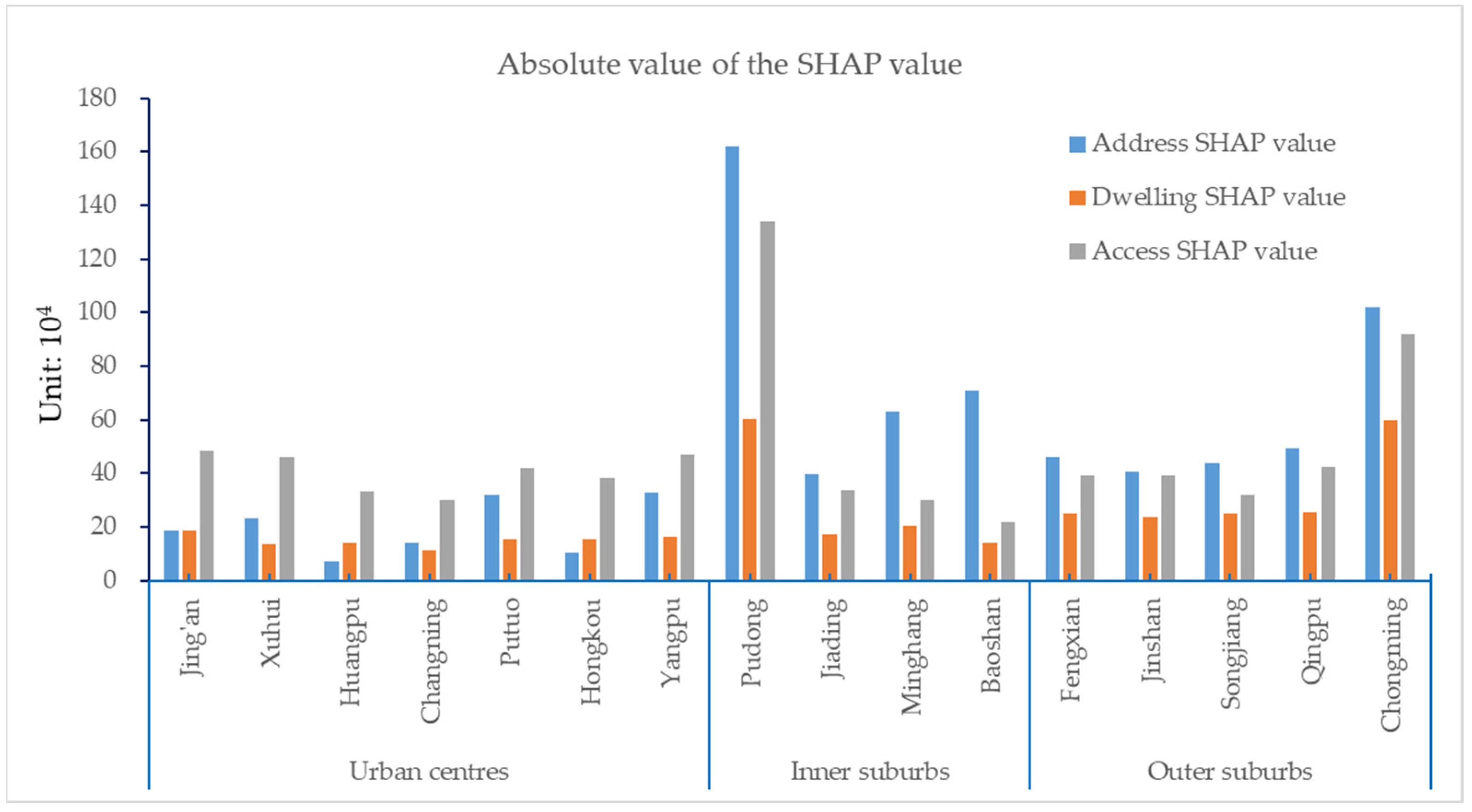
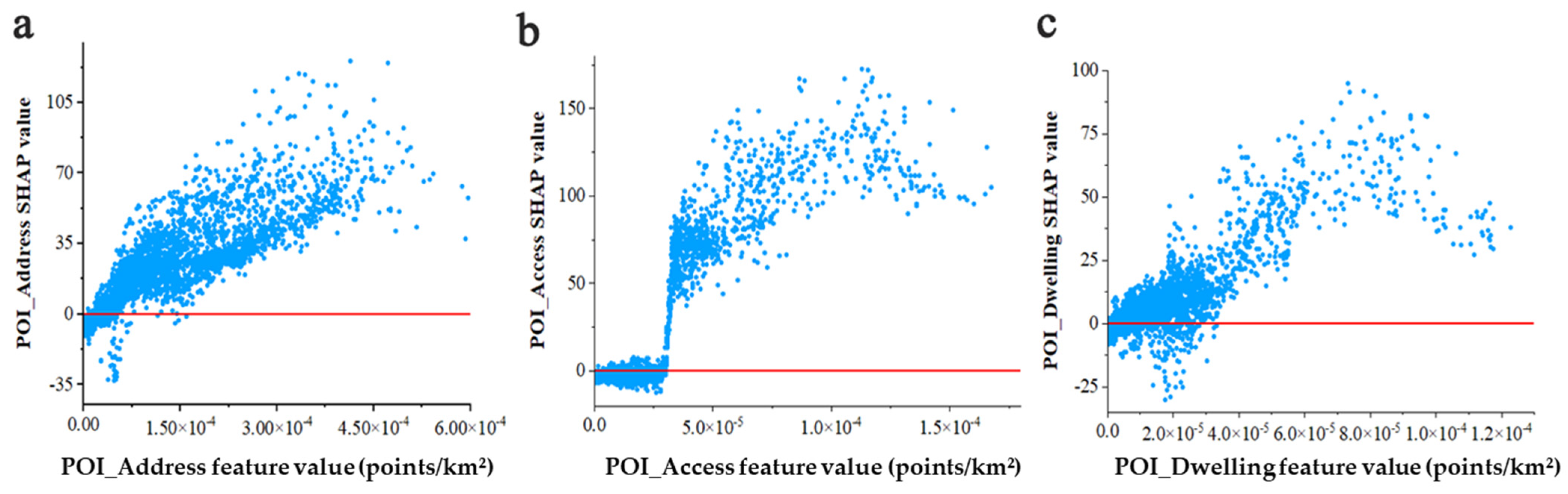
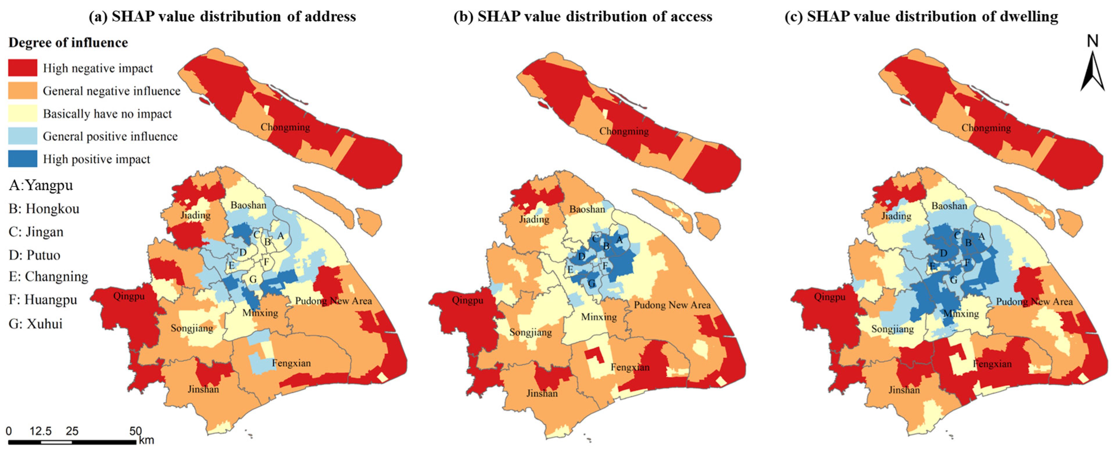
The ranking of feature variables influencing population estimation results was determined based on SHAP values. The SHAP values for address information, access facilities, and dwellings consistently rank among the top three across all districts, demonstrating stronger overall impacts on population spatialization in suburban areas than in urban centers. These features exhibit non-monotonic influences on the population estimation, revealing distinct regional variations in their effects. In urban centers, individual features show significant positive effects on the population spatial distribution. This positive influence progressively diminishes toward the suburbs, where the negative influence becomes more pronounced. The XGBoost-SHAP method effectively explains the key influencing features of population spatialization and their spatial distribution characteristics. Demonstrating strong generalizability, this approach provides a robust methodological framework for population estimation and analysis of distribution heterogeneity across cities with different typologies and varying levels of data availability;

(3)

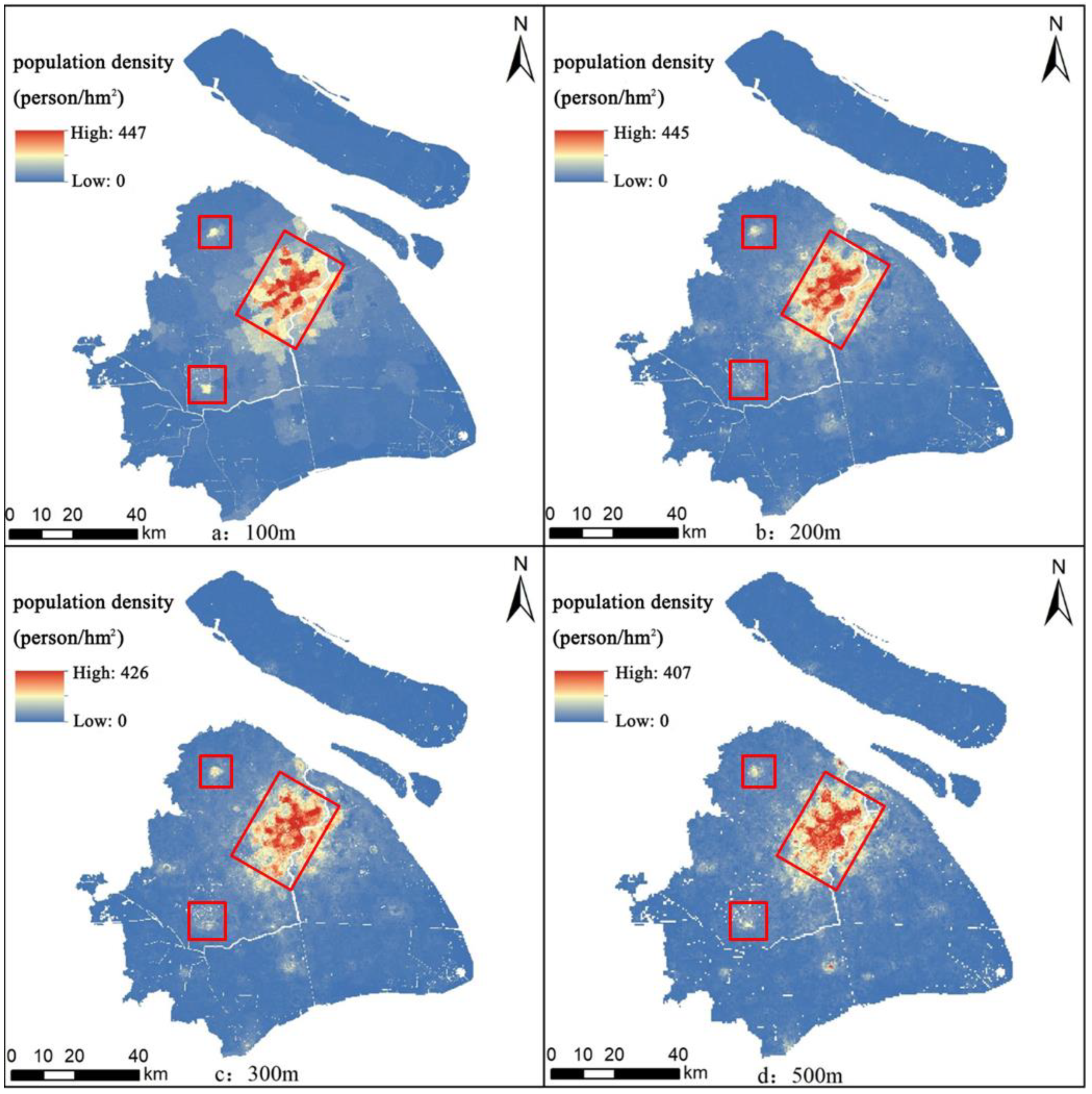
The estimated population density of Shanghai across different grid scales demonstrates consistent spatial characteristics, exhibiting a gradient decrease from the urban centers to the surrounding suburbs. Notably, as the grid scale increases, the distribution of local population density tends to become more dispersed. The comprehensive accuracy evaluation metrics and landscape ecology indices indicate that the population estimation results at the 100 m grid scale have the highest accuracy and effectively reflect the population spatial distribution heterogeneity. These findings strongly support the recommendation of 100 m as the most appropriate grid scale for population spatialization estimation in Shanghai. The high-accuracy population estimation outcomes in Shanghai facilitate the detection of latent urban development imbalances, thereby offering empirical foundations for enhancing functional district planning and the judicious allocation of spatial resources.

References

1. Li, H.; Zhang, H.; Wang, M. A comparative study of population spatialization based on NPP/VIIRS and LJ1-01 night light data: Taking Beijing for an example. Remote Sens. Inf. 2021, 36, 90–97. [Google Scholar] [CrossRef]
2. Effat, H.A.; Ramadan, M.S. Geospatial modeling for a sustainable urban development zoning map using AHP in Ismailia Governorate, Egypt. Egypt. J. Remote Sens. Space Sci. 2021, 24, 191–202. [Google Scholar] [CrossRef]
3. Xiao, D.; Yang, S. A review of population spatial distribution based on nighttime light data. Remote Sens. Land Resour. 2019, 31, 10–19. [Google Scholar] [CrossRef]
4. Wu, H.; Hu, Q.; Li, R.; Liu, C. Research progress on spatio-temporal distribution estimation of urban population. Acta Geod. Cartogr. Sin. 2022, 51, 1827–1847. [Google Scholar] [CrossRef]
5. Tatem, A.J. WorldPop, open data for spatial demography. Sci. Data 2017, 4, 170004. [Google Scholar] [CrossRef]
6. Bai, Z.; Wang, J.; Yang, F. Research progress in spatialization for population data. Prog. Geogr. 2013, 32, 1692–1702. [Google Scholar] [CrossRef]
7. Liu, A.; Zou, Z.; Liu, M. On Evolution of Metropolitan Spatial Structure Based on Population Density Models: A Case Study of Tianjin. Urban Dev. Stud. 2015, 22, 141–144. [Google Scholar]
8. Newling, B.E. The spatial variation of urban population densities. Geogr. Rev. 1969, 59, 242–252. [Google Scholar] [CrossRef]
9. Chen, H.; Quan, D.; Zhao, X.; He, J. Evolutional trends of population spatial distribution in western under-developed city—A case study of Lanzhou. World Reg. Stud. 2019, 28, 105–114. [Google Scholar] [CrossRef]
10. Langford, M. An evaluation of small area population estimation techniques using open access ancillary data. Geogr. Anal. 2013, 45, 324–344. [Google Scholar] [CrossRef]
11. Schroeder, J.P. Hybrid areal interpolation of census counts from 2000 blocks to 2010 geographies. Comput. Environ. Urban Syst. 2017, 62, 53–63. [Google Scholar] [CrossRef] [PubMed]
12. Jin, Y.; Liu, R.; Fan, H.; Li, P.; Liu, Y.; Jia, Y. Multi-Resolution Population Mapping Based on a Stepwise Downscaling Approach Using Multisource Data. Remote Sens 2023, 15, 1947. [Google Scholar] [CrossRef]
13. Huang, Y.; Zhao, C.; Song, X.; Chen, J.; Li, Z. A semi-parametric geographically weighted (S-GWR) approach for modeling spatial distribution of population. Ecol. Indic. 2018, 85, 1022–1029. [Google Scholar] [CrossRef]
14. Lwin, K.K.; Sugiura, K.; Zettsu, K. Space–time multiple regression model for grid-based population estimation in urban areas. Int. J. Geogr. Inf. Sci. 2016, 30, 1579–1593. [Google Scholar] [CrossRef]
15. Yang, R.; Dong, C.; Zhang, Y. Method of population spatialization under the support of geographic national conditions data. Sci. Surv. Mapp. 2017, 42, 76–81. [Google Scholar] [CrossRef]
16. Guo, H.; Zhu, W. A review on the spatial disaggregation of socioeconomic statistical data. Acta Geogr. Sin. 2022, 77, 2650–2667. [Google Scholar] [CrossRef]
17. Liu, Y.; Tian, T.; Gu, J.; Liu, J. Fine spatio-temporal scale estimation of urban population’s socio-economic characteristics based on big data: Data, methods and applications. Popul. Econ. 2022, 1, 42–57. [Google Scholar] [CrossRef]
18. Zhang, Y.; Wang, H.; Luo, K.; Wu, C.; Li, S. Study on Spatialization and Spatial Pattern of Population Based on Multi-Source Data—A Case Study of the Urban Agglomeration on the North Slope of Tianshan Mountain in Xinjiang, China. Sustainability 2024, 16, 4106. [Google Scholar] [CrossRef]
19. Batista e Silva, F.; Freire, S.; Schiavina, M.; Rosina, K.; Marín-Herrera, M.A.; Ziemba, L.; Craglia, M.; Koomen, E.; Lavalle, C. Uncovering temporal changes in Europe’s population density patterns using a data fusion approach. Nat. Commun 2020, 11, 4631. [Google Scholar] [CrossRef]
20. Tu, W.; Liu, Z.; Du, Y.; Yi, J.; Liang, F.; Wang, N.; Qian, J.; Huang, S.; Wang, H. An ensemble method to generate high-resolution gridded population data for China from digital footprint and ancillary geospatial data. Int. J. Appl. Earth Obs. Geoinf. 2022, 107, 102709. [Google Scholar] [CrossRef]
21. Wang, C.; Kan, A.; Zeng, Y.; Li, G.; Wang, M.; Ci, R. Population distribution pattern and influencing factors in Tibet based on random forest model. Acta Geogr. Sin. 2019, 74, 664–680. [Google Scholar] [CrossRef]
22. He, M.; Xu, Y.; Li, N. Population spatialization in Beijing city based on machine learning and multisource remote sensing data. Remote Sens. 2020, 12, 1910. [Google Scholar] [CrossRef]
23. Zhao, X.; Xia, N.; Xu, Y.; Huang, X.; Li, M. Mapping Population Distribution Based on XGBoost Using Multisource Data. IEEE J. Sel. Top. Appl. Earth Obs. Remote Sens. 2021, 14, 11567–11580. [Google Scholar] [CrossRef]
24. Chen, T.; He, T.; Benesty, M.; Khotilovich, V.; Tang, Y. Xgboost: Extreme Gradient Boosting. R package version 0.4-2. 2015; pp. 1–4. [Google Scholar]
25. Ribeiro, M.T.; Singh, S.; Guestrin, C. “Why should I trust you?” Explaining the predictions of any classifier. In Proceedings of the 22nd ACM SIGKDD International Conference on Knowledge Discovery and Data Mining, San Francisco, CA, USA, 13–17 August 2016; pp. 1135–1144. [Google Scholar] [CrossRef]
26. Lundberg, S.M.; Erion, G.; Chen, H.; Degrave, A.; Prutkin, J.M.; Nair, B.; Katz, R.; Himmelfarb, J.; Bansal, N.; Lee, S.I. From local explanations to global understanding with explainable AI for trees. Nat. Mach. Intell. 2020, 2, 56–67. [Google Scholar] [CrossRef]
27. Liu, T.; Zhang, Q.; Li, T.; Zhang, K. Dynamic Vegetation Responses to Climate and Land Use Changes over the Inner Mongolia Reach of the Yellow River Basin, China. Remote Sens. 2023, 15, 3531. [Google Scholar] [CrossRef]
28. Li, L.; Zeng, Z.; Zhang, G.; Duan, K.; Liu, B.; Cai, X. Exploring the Individualized Effect of Climatic Drivers on MODIS Net Primary Productivity through an Explainable Machine Learning Framework. Remote Sens. 2022, 14, 4401. [Google Scholar] [CrossRef]
29. Dikshit, A.; Pradhan, B. Interpretable and explainable AI (XAI) model for spatial drought prediction. Sci. Total Environ. 2021, 801, 149797. [Google Scholar] [CrossRef]
30. Li, X.; Wu, C.; Meadows, M.E.; Zhang, Z.; Lin, X.; Zhang, Z.; Chi, Y.; Feng, M.; Li, E.; Hu, Y. Factors Underlying Spatiotemporal Variations in Atmospheric PM2.5 Concentrations in Zhejiang Province, China. Remote Sens. 2021, 13, 3011. [Google Scholar] [CrossRef]
31. Luo, Y.; Dong, C.; Zhang, Y. Research on the evaluation method of population spatialization suitable grid. J. Geo-Inf. Sci. 2023, 25, 896–908. [Google Scholar]
32. GB/T 35648-2017; General Administration of Quality Supervision, Inspection and Quarantine of the People’s Republic of China, National Standardization Administration. Classification and Coding of Geographic Information Points of Interest. Standardization and Administration of the People’s Republic of China: Beijing, China, 2017.
33. GB/T21010-2017; Current Land Use Classification. General Administration of Quality Supervision, Inspection Quarantine of P. R. C. Standardization and Administration of the People’s Republic of China: Beijing, China, 2017.
34. Chen, T.; Guestrin, C. Xgboost: A scalable tree boosting system. In Proceedings of the 22nd ACM SIGKDD International Conference on Knowledge Discovery and Data Mining, San Francisco, CA, USA, 13–17 August 2016; pp. 785–794. [Google Scholar] [CrossRef]
35. Mousa, S.R.; Bakhit, P.R.; Ishak, S. An extreme gradient boosting method for identifying the factors contributing to crash/near-crash events: A naturalistic driving study. Can. J. Civ. Eng. 2019, 46, 712–721. [Google Scholar] [CrossRef]
36. Štrumbelj, E.; Kononenko, I. Explaining prediction models and individual predictions with feature contributions. Knowl. Inf. Syst. 2014, 41, 647–665. [Google Scholar] [CrossRef]
37. Lundberg, S.M.; Lee, S.-I. A Unified Approach to Interpreting Model Predictions. arXiv 2017, arXiv:1705.07874. [Google Scholar] [CrossRef]
38. Shapley, L.S. A value for n-person games. Contrib. Theory Game 1953, 2, 307–317. [Google Scholar] [CrossRef]
39. Bao, W.; Gong, A.; Zhao, Y.; Chen, S.; Ba, W.; He, Y. High-Precision Population Spatialization in Metropolises Based on Ensemble Learning: A Case Study of Beijing, China. Remote Sens. 2022, 14, 3654. [Google Scholar] [CrossRef]
40. Yeh, C.-T.; Huang, S.-L. Investigating spatiotemporal patterns of landscape diversity in response to urbanization. Landsc. Urban Plan. 2009, 93, 151–162. [Google Scholar] [CrossRef]
41. Gaughan, A.E.; Stevens, F.R.; Huang, Z.J.; Jeremiah, J.N.; Sorichetta, A.; Lai, S.J.; Ye, X.Y.; Linard, C.; Hornby, G.M.; Hay, S.I.; et al. Spatiotemporal patternsof population in China’s mainland, 1990 to 2010. Sci. Data 2016, 3, 160005. [Google Scholar] [CrossRef] [PubMed]
42. Zhao, S.; Liu, Y.; Zhang, R.; Fu, B. China’s population spatialization based on three machine learning models. J. Clean. Prod. 2020, 256, 120644. [Google Scholar] [CrossRef]
43. Song, Y.; Wu, S.; Chen, B.; Bell, M.L. Unraveling near real-time spatial dynamics of population using geographical ensemble learning. Int. J. Appl. Earth Obs. Geoinf. 2024, 130, 103882. [Google Scholar] [CrossRef] [PubMed]
44. Guo, W.; Zhang, J.; Zhao, X.; Li, Y.; Liu, J.; Sun, W.; Fan, D. Combining Luojia1-01 nighttime light and points-of-interest data for fine mapping of population spatialization based on the zonal classification method. IEEE J. Sel. Top. Appl. Earth Obs. Remote Sens. 2023, 16, 1589–1600. [Google Scholar] [CrossRef]
45. Zhang, J.; Zhao, X. Using POI and multisource satellite datasets for mainland China’s population spatialization and spatiotemporal changes based on regional heterogeneity. Sci. Total Environ. 2024, 912, 169499. [Google Scholar] [CrossRef]
46. Huang, D.; Yang, X.; Dong, N.; Cai, H. Evaluating grid size suitability of population distribution data via improved ALV method: A case study in Anhui Province, China. Sustainability 2017, 10, 41. [Google Scholar] [CrossRef]
47. Ge, M.; Feng, Z. Study on the distribution pattern of China’s population in 2000 based on GIS: Comparison with Hu Huanyong’s research in 1935. Popul. Res. 2008, 32, 51–57. [Google Scholar]
48. Balk, D.L.; Deichmann, U.; Yetman, G.; Pozzi, F.; Hay, S.I.; Nelson, A. Determining Global Population Distribution: Methods, Applications and Data. Adv. Parasitol. 2006, 62, 119–156. [Google Scholar] [CrossRef] [PubMed]
49. Tobler, W.; Deichmann, U.; Gottsegen, J.; Maloy, K. World population in a grid of spherical quadrilaterals. Int. J. Popul. Geogr 1997, 3, 203–225. [Google Scholar] [CrossRef]
50. Dobson, J.E.; Bright, E.A.; Coleman, P.R.; Durfee, R.C.; Worley, B.A. LandScan: A global population database for estimating populations at risk. Photogramm. Eng. Remote Sens. 2000, 66, 849–857. [Google Scholar]
51. Dong, N.; Yang, X.; Cai, H.; Xu, F. Research on grid size suitability of gridded population distribution in urban area: A case study in urban area of Xuanzhou district, China. PLoS ONE 2017, 12, e0170830. [Google Scholar] [CrossRef]
52. Ye, J.; Yang, X.; Jiang, D. The grid scale effect analysis on town leveled population statistical data spatialization. J. Geo-Inf. Sci. 2010, 12, 40–47. [Google Scholar] [CrossRef]
53. Wu, J.; Gui, Z.; Shen, L.; Wu, H.; Liu, H.; Li, R.; Mei, Y.; Peng, D. Population spatialization by considering pixel-Level attribute grading and spatial association. Geomat. Inf. Sci. Wuhan Univ. 2022, 47, 1364–1375. [Google Scholar] [CrossRef]
Figure 1. SHAP diagram ranking the importance of feature variables.
Applsci 15 04755 g001
Figure 2. SHAP values of main feature variables in different districts of Shanghai.
Applsci 15 04755 g002
Figure 3. Accuracy of population estimation results. (a) Correlation between census population and estimated population (b) Correlation between WorldPop and estimated population.
Applsci 15 04755 g003
Figure 4. SHAP feature dependency graph. (a) The SHAP value corresponding to the address feature; (b) The SHAP value corresponding to the access feature; (c) The SHAP value corresponding to the Dwelling feature.
Applsci 15 04755 g004
Figure 5. Distribution of SHAP values for address information, access facilities, and dwellings at town and street scales.
Applsci 15 04755 g005
Figure 6. Spatial distribution of population density at different grid scales.
Applsci 15 04755 g006
Figure 7. Heterogeneity evaluation of population spatial distribution at different grid scales.
Applsci 15 04755 g007
Figure 8. Spatial distribution of DN and POI kernel density.
Applsci 15 04755 g008