A Solution for Predicting the Timespan Needed for Grinding Roller Bearing Rings

Abstract

The optimal management of manufacturing processes can be achieved through a set of optimal decisions, which must be made to choose the best method to follow every time the process planner reaches a point when several potential manufacturing paths branch off. A dedicated method, namely the Holistic Optimization Method (HOM), has already been developed for this purpose and has been validated in several studies based on artificial- and real-instance databases. The HOM consists of two algorithms: (i) the causal identification of a manufacturing process and (ii) a comparative assessment with similar already-assessed manufacturing cases recorded in an instance database. The two algorithms can be used to estimate the values of the different performance indicators of manufacturing processes. Their application for processing cost estimation in the case of the manufacturing processes of bearing components has already shown good results. In this paper, the HOM is presented as a solution for predicting the timespan needed for grinding roller bearing rings. The specific algorithms of the HOM were applied, grounded in the use of a database with data collected from the industrial environment. The cause variables selected to describe the grinding process of the roller bearing rings were the inner and outer diameter of the ring, its width and weight, the machined surface roughness, the grinding stone rotation speed, the cutting speed, the feed rate, and the cutting depth, while the effect variable to be used by the process planner as the decision criterion was the timespan.

1. Introduction

In the current economic environment, industrial manufacturers have defined and implemented different development strategies based on cost-efficiency principles, considering, on one hand, resource availability and rational consumption and, on the other, production parameter improvement through a lead time reduction under conditions of keeping the same quality of the produced and delivered goods. Customer behavior has become focused on finding and qualifying suppliers, which are more suited to providing a quick reply to a customer’s request, even in terms of a quotation, but more importantly, after the confirmation of a firm order, it has become a trend to predict the production cost and lead time using the data collected on formerly closed orders [1].

In recent years, companies have sought to increase their profits by investing resources in both the creation of new products and the discovery of new methods of manufacturing and delivering existing products [2].

The use of past knowledge collected during the product production stages (namely order acceptance, production planning, product design, process planning, product processing, and product delivery) is considered a key factor for improving manufacturing performance in the modern manufacturing industry [3]. In the quotation phase, the supplier should be able to predict with good accuracy the final answer in order to respond to diversified customer needs [4]. For this purpose, both the input data from the potential customer (i.e., the requested quantity of goods, the requested delivery date, and the quality of the goods) and the production lead time, considering the production flow and necessary resources, must be considered.

In a real-life manufacturing processes, such as the grinding of some bearing components, the accumulation of sufficient data [5] for making timespan predictions may take a long time, during which the initial conditions (production mix, orders, process parameters, and so forth) may change. The processing of the collected data by some empirical methods involves a great deal of time and the results may be affected by potential errors; meanwhile, a certain delay in answering customers could occur. In order to eliminate as much as possible the mentioned weakness related to time measurement and data processing, suppliers should focus more on the development of programs or dedicated applications that are able to predict the correlation between different factors of the production process (timespan, production range, technical specification for the products, machine availability, and productivity) and the order delivery deadline, based on a database which contains information gathered from previous closed orders and by using a real-world manufacturing process [4]. Under these circumstances, companies that use knowledge collection based on recorded and processed data concerning their products and ongoing processes, and which can apply it effectively and efficiently, will be successful at achieving competitive advantages [6].

The economy of machining operations plays a key role in competitiveness in the market. The authors addressed the minimization of the production time of a cutting process in [7]. They determined the optimal processing parameters in the case of processing a continuous profile in relation to the production time. The lead time is a central element of the economic evaluation of a newly ordered or only quoted product [8]. A cost breakdown helps the process engineers understand the main cost components and also observe the main influences of the process parameters, such as the timespan, cutting speed, feed rate, and cutting depth, on the final cost of the product during the quotation phase [9]. The manufacturing process between ordering and product delivery involves two successive stages that are time-consuming and have an impact on the results—the production cost and the delivery time. At each stage, before a firm order is placed and accepted, both the customer and the supplier should consider the entire decision-making process related to the transformation of the raw material into a semi-finished product and finally into a product, and they should be involved in all the successive stages of the manufacturing chain (ordering, design, planning, programming, and processing), including the allocation of resources [10].

The decisions that are currently made in manufacturing management are based on a “what if” analysis [11]. This analysis requires models that express the connection between the decision parameters and the results of the manufacturing process. In the current approaches, these models are generally analytical, and the evaluation of the results is direct.

The activities performed during the manufacturing process (which include the following stages: bidding–negotiating–acceptance of the order, product design, process planning, and job scheduling) have different natures; at the same time, their exigencies are diverse [12]. The effect variables of a certain activity, which should be used to evaluate a given effect from the process end, are not precisely known; moreover, they must be selected from a set of measurable variables specific to the activity, which are not necessarily independent. The causal relationships either between the cause variables or between the cause variables and the effect variables are not known a priori. The possible existence of a high number of jobs needed to obtain the product involves too large a number of variables to be managed—the dimensionality of the problem to be solved is too large for existing computational resources.

In modern manufacturing, the volume of data is growing at an unprecedented level and these huge amounts of data in manufacturing databases, which contain large numbers of records, with many attributes that need to be simultaneously explored to discover useful information and knowledge, make manual analysis impractical [13]. Some dedicated solution based on specific algorithms that use the collected data from the industrial environment and could become important tools for processing of data, information, and knowledge automatically from manufacturing databases [13] could be developed in existing and future manufacturing and commercial environments.

The real challenge is to identify a solution that can help the manufacturers to predict rapidly and with great accuracy the indicators of a given manufacturing process based on collected data and knowledge. A possible answer to this challenge has already been provided by the development of the HOM [12]. Applications of this method are presented in some of our previous works. Thus, in [14], the cost in the case of bearings with interchangeable construction was evaluated. Furthermore, in [9], the manufacturing costs of the roller bearings were estimated.

This paper presents a solution that predicts the timespan needed for the grinding of roller bearing rings based on the use of a database with data collected from the industrial environment by applying the specific algorithms of the HOM. The HOM includes two algorithms: (i) the causal identification of a manufacturing process and (ii) the comparative assessment among the already performed manufacturing cases, recorded as an instances database. The two algorithms can be used to estimate the values of different performance indicators of the processing processes. The solution presented in this study is characterized by the fact that a decision must be made at any time during the manufacturing process by using both proposed algorithms. The first proposed algorithm is based on a causal model which is used to link the decision parameters to the results. The second proposed algorithm is developed based on the principle of comparative assessment among the already performed manufacturing cases, recorded as an instances database.

The case study developed in this paper for timespan prediction in the manufacturing process of grinding roller bearing rings is validated based on a database with data collected from the industrial environment.

The decision to emphasize this specific indicator, timespan, came from its critical role in production management. Production management involves the scheduling of all resources considering overall operational efficiency within the industry. Timespan prediction directly impacts scheduling, resource allocation, and delivery timelines. Delays in job completion can lead to increased costs and energy consumption. This study was developed with the purpose of addressing timespan prediction as a fundamental aspect that can influence the performance of manufacturing processes.

The paper is organized as follows: Section 2 presents the grinding roller bearing rings process. Section 3 describes the two algorithms of the HOM for timespan prediction; namely, the causal identification and the comparative assessment. Section 4 is dedicated to the results of the application of the two algorithms to the case of timespan prediction for grinding roller bearing rings using a database with data collected from the industrial environment. Section 5 presents the paper’s conclusions.

2. Manufacturing Process for Bearing Rings

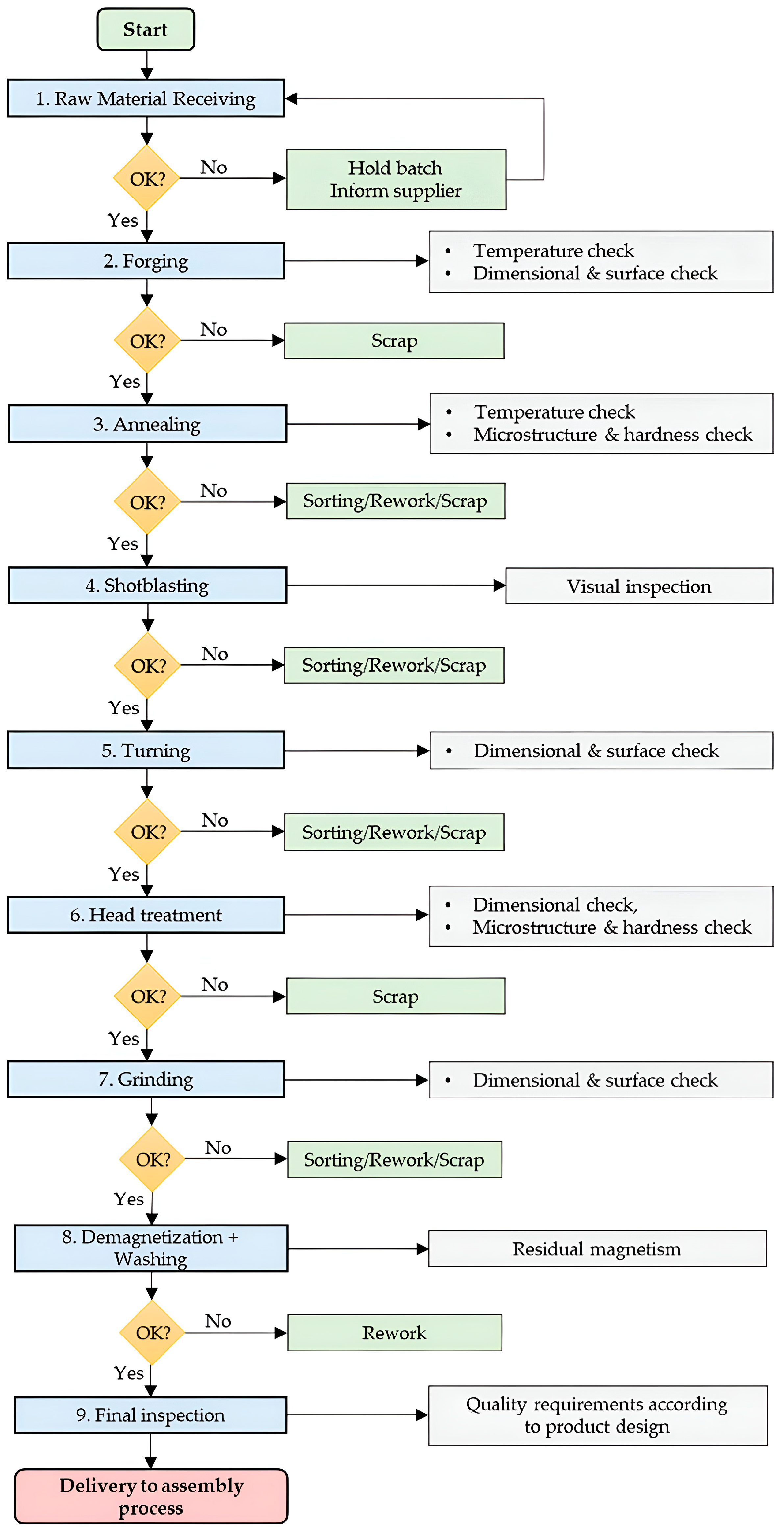
2.1. The Identification of the Flow Diagram for the Manufacturing of an Inner and Outer Bearing Ring

Bearings are the most common machine parts [15] and have extensive applications in industrial fields, such as the railway, automotive, aeronautical, and machine tool manufacturing industries.

In order to obtain a bearing which is suitable for the intended usage, the manufacturing process should be under control from both the process and product parameters.

The designed process parameters are dedicated for each process step and the setting up of these parameters on machine tools involves some activities that are time consuming.

The collection and usage of the values of the set-up parameters and the measured process and product parameters in a database, which could be used as a reference for future orders, quotations or in some improvement strategies, becomes necessary in the actual manufacturing environment and also in the transfer of knowledge between employees.

To be able to follow products in the production field and to assure the traceability of products, process, measurements, and decisions to be taken in bearings manufacturing processes, one of the most important steps is to identify flow diagrams and then, based on these documents, compile the operation and verification plans for each process step and phase.

Figure 1 presents the generic flow diagram for the manufacturing of inner and outer bearing rings, as well as the manufacturing processes used to produce bearing components. To manufacture a conforming bearing component, each step of the process must be defined, designed, implemented, and controlled during production. The main production steps, starting from raw material reception, are as follows: the forging of rings, this process is controlled by checking temperature and dimensions of the produced sample; the annealing process, which is controlled through the temperature, time, and microstructure of the sample; the shot blasting process, which is controlled through process time and surface quality by visual inspection; turning, controlled through process parameters, set-up parameters, dimensions, visual inspection, and surface quality; secondary heat treatment (quenching and tempering), controlled through temperature, time, microstructure and the hardness of the sample; the grinding process, characterized through process parameters, set-up parameters, and, for the obtained product, through geometrical and shape deviation control and surface aspect control; the demagnetization process, controlled through process time and remanent magnetism; and the washing process, controlled through the degree of cleanliness of the product. The final inspection, before the assembly of the bearings, involves complete measurements of the product parameters and a visual inspection. From the generic flowchart depicted in Figure 1, which applies to the manufacture of bearing rings, the grinding process was selected for this research. This process plays an important role in geometrical and shape deviations, surface quality, and, ultimately, bearing function. It is known that the geometrical and surface parameters requested for bearing components are strongly related to the bearing’s main application. To produce components within the technical requirements, the grinding process should be controlled from both the process control and the product parameter control perspectives. Considering the relationship between process parameters and product parameters, this paper presents data collected from an industrial manufacturer in the bearing production industry. A set of parameters specific to the grinding process, such as the inner and outer diameter of the ring, its width and weight, the machined surface roughness, the grinding stone rotation speed, the cutting speed, the feed rate, and the cutting depth, were considered as input data for the proposed application of the HOM. The database was then used to apply the HOM to predict and optimize the process in terms of timespan. The timespan prediction is an important indicator in different phases of a manufacturing process and gives important information for production scheduling and production lead time.

In the present study, the grinding process, namely step 7, from the flow diagram (see Figure 1) was selected to identify the process parameters for predicting the timespan in case of cylindrical roller bearing rings with the help of the two algorithms—namely, causal identification and comparative assessment—presented in the next chapter.

2.2. Grinding Operations

Presently, grinding processes are widely used industry [16]. Grinding is one of the most important and common processes [17] for the production of components and parts with high precision and quality [18]. Consequently, the accuracy of this process is very important in order to ensure the final quality of the product. Current data collection and inspection technologies allow for data to be collected online along the process chain, and can significantly increase quality control and can result in improvements in current dynamic and modifiable environments [19]. The real challenge facing companies is the problem of synthesizing highly heterogeneous data to gain an in-depth understanding of the correlations between the variables throughout the stages of a multi-stage system; the goal being the generation of zero defects at the process level and zero defects at the system level through the proactive control of the process.

In a manufacturing process, different processing phases for grinding can be identified. These phases are performed successively considering the allowance material and the values of the technical parameters to be obtained after each phase. The main phases were synthetized as the rough grinding phase, the fine grinding phase [20], and the superfinishing grinding phase. In case of a bearing ring, the process phases are performed according to the designed role of the surface. For example, in the case of an inner ring, the last stage is fine grinding for the surface of the inner diameter. In the case of an outer ring, fine grinding is the last phase for the outer ring surface. Meanwhile, for both types of rings, in the case of raceway surfaces, the last stage is superfinishing due to the designed surface texture, which is defined in terms of surface roughness, waviness, lay, and flaws, and is concerned with the geometric irregularities of the surface [21] and profile. The grinding process is one of the most important processing methods widely used in the manufacture of bearings [22]. The control and the optimization of this process could have a great impact on the final results, such as the bearings’ clearances, and subsequently on the function of the bearing as a part of a machine or other system. A multi-objective optimization method for reducing the grinding time and material removal rate by applying the genetic algorithm NSGA-II and the Pareto set was proposed in [22].

A new evolutionary computation technique, namely particle swarm optimization, which optimizes grinding process parameters (such as wheel speed, workpiece speed, the depth of dressing, and the lead of dressing) and that will minimize the unit production cost and time with the finest possible surface finish, was developed by the authors of the study presented in [23].

3. Method for Timespan Prediction

The HOM has already been developed for this purpose and has been validated in several studies based on artificial- and real-instance databases. The novelty of the method lies in using a numerical model of the process (an instances database) instead of other types of models (analytical, convolutional, neural, etc.) and in its evaluation of the value of the output variable by comparing among the cases from the database (by considering the “causal distance”) instead of directly calculating it. The HOM consists of two algorithms: (i) the causal identification of a manufacturing process and (ii) the comparative assessment with similar already-performed manufacturing cases, recorded in an instances database. The two above-mentioned algorithms will be further presented in detail.

3.1. The Causal Identification Algorithm

The causal identification algorithm allows for multiple forms to be provided for one and the same causal relationship. This is designed to be applied in the case of a manufacturing process before the comparative assessment of the results of the activities that can be selected at the level of a decision point in the manufacturing process graph [12].

It allows for the identification of the most appropriate set of cause variables, based on which an effect variable can be evaluated, depending on the specific conditions of a particular manufacturing process.

The final purpose of this algorithm is to elaborate the tree of causal links, which can be considered a system of decision-making (“Decision Support System, DSS” [24]).

Figure 2 shows the causal identification algorithm of a manufacturing process. The meanings of the abbreviations presented in Figure 2 are: h_ref—the reference threshold for selection of cause variables that model the effect variable and its value, depending on the number of beams available in the database; MP, MC, and MU—the values of the modeling capacity criteria in the case of evaluating a causal variable; a (which corresponds to the value of the modeling power criterion, MP), b (which corresponds to the value of the modeling capacity criterion, MC), RMSE (Root Mean Square Error, which corresponds to the value of the modeling unevenness criterion, MU)—the values of the criteria used to evaluate the cluster potential; ∆C and ∆M—the values of the results obtained using the Curve fitting tool, which is necessary for the graphic exemplification that underlies the evaluation of the characteristics in the case of cause and effect variables; MP_c, MC_c, and MU_c—the values of the modeling capacity criteria when evaluating the sets of causal variables; a_c and b_c—the regression coefficients where a_c is the slope of the regression line that corresponds to the value of the MP_c criterion and b_c is the free term of the regression line, which corresponds to the value of the MC_c criterion; and RMSE—which corresponds to the value of the MU_c criterion.

The use of the first-decision block illustrated in Figure 2 pertains to the selection of the cause variables used in cluster formation. In Figure 2, ∆_min is the image dimension (the dimension of the variable under investigation), while h_k−1 represents the previous threshold. If Δ_min is less than h_k−1, then the cause variable corresponding to Δ_min can be considered as highly dependent on other cause variables, and it may be eliminated. The remaining set of cause variables is repetitively submitted to the three previous actions until the current value of Δ_min becomes higher than h_k−1. The final set of cause variables constitutes the maximal cluster of variables. These cause variables can be considered relatively independent of each other and can be used to model the effect variable. The role of the second decision block shown in Figure 2 is to stop the iterative generation of smaller sets, when the value(s) for one or more modeling capability characteristics fall below a predefined threshold value, which indicates that the sets become unable to describe the effect variable satisfactorily.

Before defining the steps of the algorithm shown in Figure 2, an initial process identification is necessary. In this stage, the variant of the target manufacturing process is analyzed to find the variables that characterize its realization. Also, at this initial process identification stage, the set of variables (both cause and effect variables) with potential in process modeling is defined. A database containing both types of variables is built.

This algorithm involves the following five steps:

A.

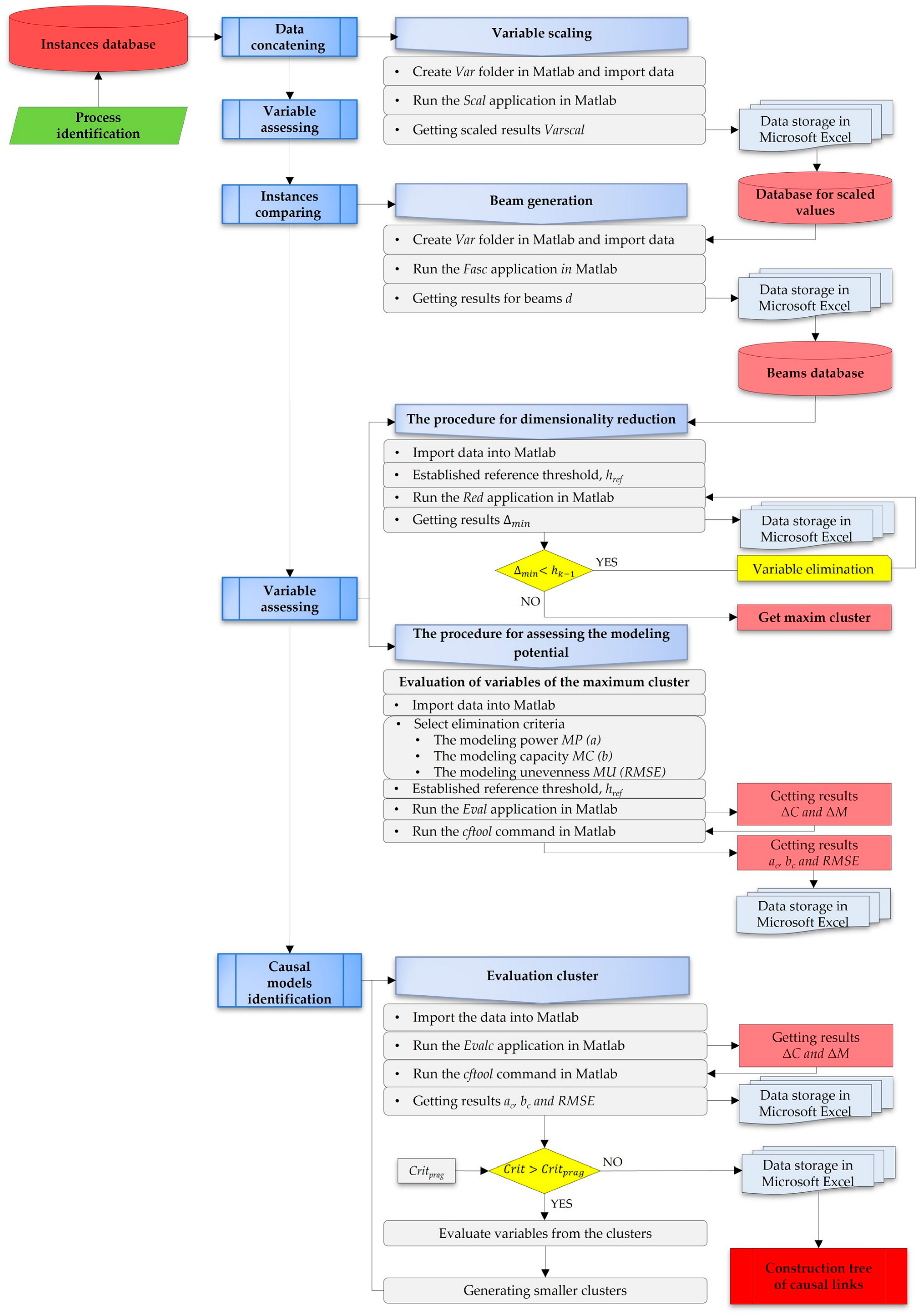
The first step involves data concatenation—for this purpose, data stored in a database are selected. In addition to selecting the data related to the manufacturing activity which is being analyzed, it is necessary to scale the variables to values between 1 and 0. To achieve this variable scaling, a MATLAB R2018a application (Scal) was developed. After running the scaling algorithm, the scaled values (Varscal) of the variables must be stored; for example, in a new file in Microsoft Excel.

B.

The second step means instance comparison—which proposes the generation of data beams. The causal identification methods start from the premise that the relevance of a cause variable to the effect variable and the modeling of the effect variable is directly related to the degree to which variation in the cause variable is found in the variation in the effect variable. Based on the value lines in the case database, the beams result from the difference between the homologous variables from different lines. To achieve beam generation, a MATLAB application (Fasc) was developed. After running the beam algorithm, the beam values (d) of the variables must be stored; for example, in a new file in Microsoft Excel.

C.

The third step is variable assessment—which involves two actions [11]; namely, problem dimensionality reduction and modeling capability assessment. The problem dimensionality reduction aims to eliminate the cause variables that have a redundant effect on the effect variable.

For the modeling capability assessment, the following three indicators were defined:

• Modeling power MP, which indicates how much of the variation in the cause variable is reflected in the variation in the effect variable;
• Modeling capacity MC, which measures the extent to which the cause variable is capable to describing the effect variable alone;
• Modeling unevenness MU, which reflects the dispersion of effect variable values when the cause variable exhibits uniform variation.

The original MATLAB applications were designed for both problem dimensionality reduction (Red) and modeling capability assessment (Evalc).

D.

The fourth step is causal model identification, which is used to determine the sets of cause variables that can be effectively used to evaluate the effect variable. This step is conducted by assessing an indicator similar to those evaluated in the individual case. For this purpose, a controlled variation is applied simultaneously to all the variables in the set and the impact on the effect variable is observed.

E.

Finally, the causal model tree is elaborated. This is the representation of causal models concerning the same effect variables. The tree results after the identification of the whole set of causal models concerning the addressed effect variable [11].

3.2. The Comparative Assessment Algorithm

The comparative assessment algorithm proposes an approach in the analysis of potentially optimal solutions when selecting between two or more process alternatives. It is based on finding rankings, according to a certain criterion, such as cost, timespan, and energy consumption. It is designed to assist the selection of the optimal continuation variant for the manufacturing process at a certain decision level. The application of this algorithm is performed after the causal identification has been completed; that is, after the adoption of a set of cause variables describing the effect variable of interest at the current moment.

Figure 3 presents the comparative assessment algorithm for the output of the manufacturing process.

The meanings of the abbreviations presented in Figure 3 are: ε—the nearness degree of the cases from a given neighborhood; x, y, and z—the scalar values of the cause variables of the current case; x_v, y_v, and z_v—the scalar values of the cause variables of the pivot case; T_v—the scalar value of the effect variable of the pivot case; ∆x, ∆y, ∆z, and ∆T—the coordinate differences; N_i—the neighborhood delimitation; mdl—the nonlinear multiple regression; P_i—the parameter vector; and α, β, γ, A, B, and C—the parameters of the proximity function.

The decision block depicted in Figure 3 supports the identification of the nearness vectors and function. The algorithm runs until P_i = P_i−1 and the current case has the minimum nearness compared to the pivot case selected for the model.

A key role in the application of the algorithm is played by the so-called “nearness function”—with the help of which the nearness between two cases is evaluated.

This algorithm involves two main procedures:

• The neighborhood delimitation procedure—which aims to find the profile of the neighborhood of a potential case through successive comparisons with cases of processes already performed (with known results).
• The nearness modeling procedure—which aims to ensure that, after delimiting a neighborhood, the nearness between its instances is modeled to find an improved form of the proximity function. For modeling, nonlinear multiple regression has been adopted as the general typology of the nearness function. The algorithm (Comp) of the method was implemented with the help of MATLAB software.

The two procedures are executed successively until the structure and form of the nearness function stabilizes. To establish a concrete case, a pivot case is selected from the database of previous cases.

The steps that must be followed to predict the timespan by applying the HOM are:

• Building the database;
• Performing the causal identification;
• Selecting a case to model for the comparative assessment;
• Selecting a pivot from the database to use in the case for which we want to make the estimation;
• The two procedures of the comparative assessment algorithm are applied until the shape of the nearness modeling functions stabilizes. Based on the final form of this function, the distance between the values of the effect variable in the pivot case and in the analyzed case is calculated. This results in the value of the effect variable in the analyzed case.

4. Results and Discussion

4.1. Database Building

A simulation of the grinding phase’s correlation with the timespan was developed in order to identify the most suitable set of cause variables with the most important impact on the timespan.

Starting from a turned piece, it is corrected through grinding phases in terms of its ovality, conicity, profile, and roughness. Considering that the influence of the mentioned parameters related to grinding phases results in the timespan of the bearing, it is important to develop simulations of the cause variables’ impact on the timespan.

The flow diagram in Figure 4 presents the step of the implementation of the HOM with the purpose of predicting the timespan needed to grind the roller bearing rings.

The flowchart depicted in Figure 4 shows a general flow of activities in different situations occurring in the industry. There are two different cases to analyze and the HOM is applied as follows:

-

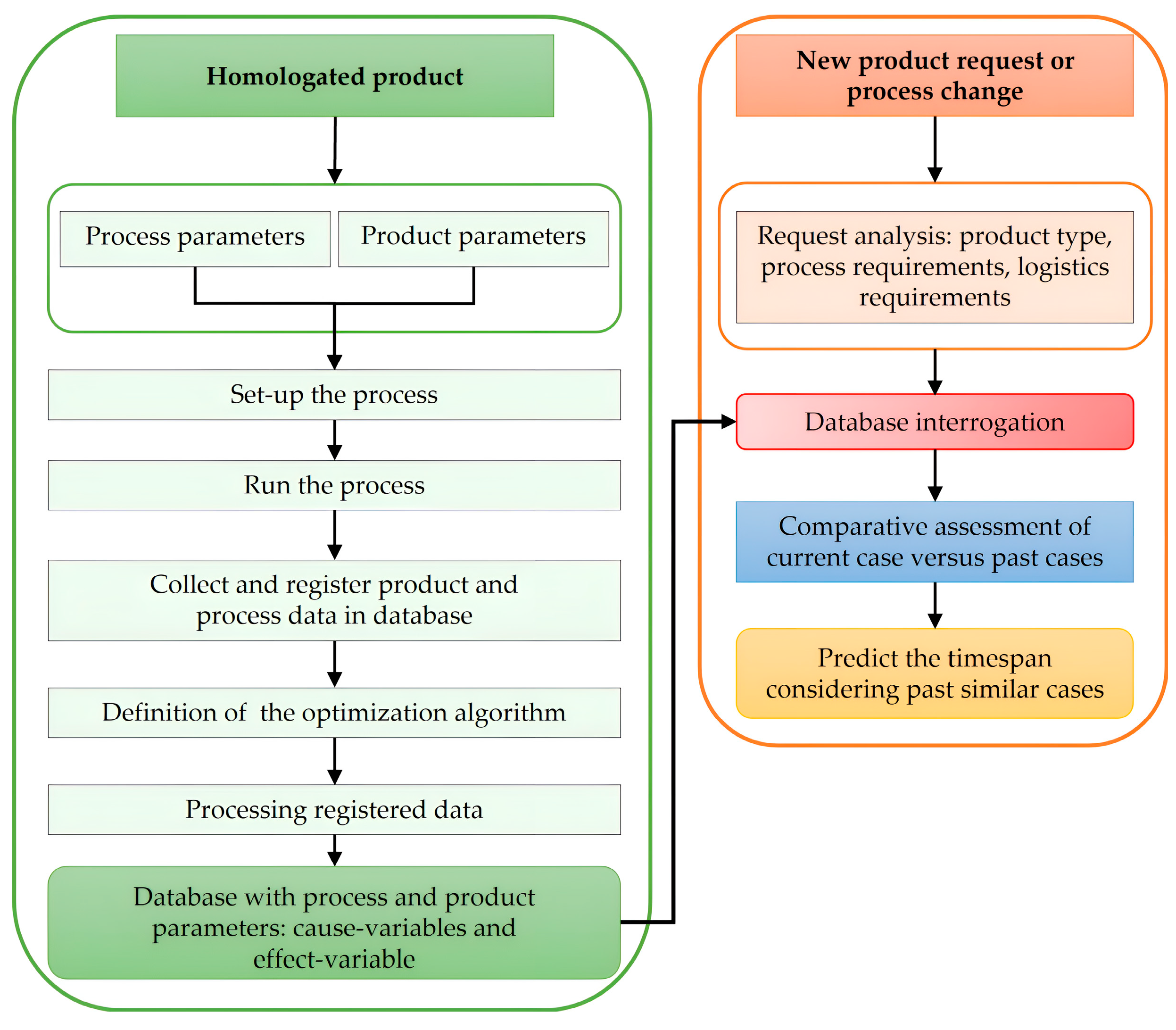
In the case of homologated products, both process and set-up parameters are known, and each run of the process will result in a new line in the database. Based on the registered data, an optimization algorithm can be defined, and cause and effect variables can be identified. A key result from the sequences of the flow diagram is the updated database.

-

In the case of a new product or a process change (process changes may occur due to an accidental defect or a lack of competencies to run the process under normal conditions), the optimization objectives could include the response time to customer requests during the quotation phase and the lead time in case of process changes according to the above details. By interrogating the database and applying the HOM, a prediction of the timespan can be obtained. In this manner, the obtained solution will help process engineers to minimize the analysis time and the lead time is therefore optimized.

4.2. Example of Timespan Prediction

To apply the HOM to the case of the grinding of roller bearing rings, the algorithms for causal identification and comparative assessment described in Section 3 were followed. The data used in the simulations were collected from the production process of some radial roller bearing rings. The set-up parameters registered are the outer diameter of the ring, D_e; the inner diameter of the ring, D_i; the width of the ring, l; the weight of the ring, g; the machined surface roughness, R_a; the cutting speed, v_a; the feed rate, f; the grinding stone rotation speed, v_r; and the cutting depth, t. The above data were input data for the simulation tests. The set-up parameters used for the grinding machine tool set-up were recorded during the normal grinding process in a manufacturing workshop. Thus, the required instances database was obtained.

4.2.1. The Application of the Algorithm for Causal Identification

The results obtained after the application of the algorithm for causal identification are described in the following, and are identical to the steps of the algorithm described in Section 3.1.

A. 

Data concatenation

The database has 77 lines, with some of them being presented, for example, in

Table 1. The real instances database (excerpt).

Instance Crt. no.	De [mm]	Di [mm]	L [mm]	g [kg]	Ra [μm]	va [m/min]	f [mm/rot]	vr [m/min]	t [mm]	Ts [min]
1	215.5	204.5	22	0.6265	0.55	28.01	0.151	79.1	0.13	0.65
2	381.3	360.05	38.15	4.264	1.61	25.06	0.91	70.02	0.6	4.765
3	250.8	237	24.7	0.9452	0.58	28.2	0.152	79.4	0.151	0.75
4	126.1	85.75	24.9	0.88	0.59	24.2	0.08	20.05	0.1501	0.29
5	240.6	220.05	38.16	2.5935	0.611	60.01	0.04	32.01	0.02	0.425
. . .	. . . . . . . . . . . . . . .

and

Table 2. The instance database (scaled values, excerpt).

Instance Crt. No.	De [mm]	Di [mm]	l [mm]	g [kg]	Ra [μm]	va [m/min]	f [mm/rot]	vr [m/min]	t [mm]	Ts [min]
1	0.293063	0.312575	0.130277	0.032378	0.290541	0.2722739	0.1315217	0.4923346	0.1582915	0.025251
2	0.590249	0.60881	0.27659	0.279543	1	0.2053956	0.9565217	0.4166806	0.748744	0.198143
3	0.356336	0.374469	0.154738	0.054033	0.310811	0.2765813	0.1326087	0.4948342	0.184673	0.029453
4	0.13282	0.086423	0.15655	0.049603	0.317568	0.1858989	0.0543478	0.0003333	0.183543	0.010126
5	0.338053	0.342189	0.276681	0.166034	0.331757	0.9977329	0.0108696	0.0999833	0.020101	0.015798
. . .	. . . . . . . . . . . . . . .

, before and after scaling, respectively.

B. 

Comparison of instances

The beam database was obtained by using a MATLAB application designed for this purpose, by comparisons between the 77 instances from the database, as explained in Section 3 and Section 3.1. Hereby, $N=C_{77}^2=2926$ beams compose the beams database. Examples of beams are shown in

Table 3. The beams database (excerpt).

Instance Crt. No.	δDe [mm]	δDi [mm]	δl [mm]	δg [kg]	δRa [μm]	va [m/min]	δf [mm/rot]	δvr [m/min]	δt [mm]	δTs [min]
1	0.297186	0.296235	0.146313	0.247165	0.709459	0.066878	0.825	0.075654	0.590452	0.172892
2	0.063273	0.061894	0.024461	0.021655	0.02027	0.004307	0.001087	0.0025	0.026382	0.004202
3	0.160244	0.226152	0.026273	0.017225	0.027027	0.086375	0.077174	0.492001	0.025251	0.015125
4	0.04499	0.029614	0.146403	0.133656	0.041216	0.725459	0.120652	0.392351	0.138191	0.009453
5	0.117315	0.179207	0.362384	0.042624	0.236486	0.432782	0.055435	0.507499	0.037688	0.063023
. . .	. . . . . . . . . . . . . . .

.

C. 

Variables assessing

At first, the reference threshold (see Section 3.1) was set to h_ref = 0.1342, hence h_k−1 = h₆ = 0.2621.

C.1. 

Dimensionality reduction

According to the algorithm in Section 3.1, at Step 1, windows of H = 0 and h = h_ref were considered for the beam components corresponding to eight of the nine cause variables, while for the nineth, the image dimension Δ_i was measured (i = 1, 2, …, 9).

Table 4. Images dimension of Δ_i and Δ_min.

Cause Variables	Successive Steps for Dimensionality Reduction
	Step 1	Step 2	Step 3	Step 4
De	0.1433	0.1433	-	-
Di	0.1705	0.1705	0.6869	0.6869
l	0.1753	0.3352	0.3352	0.6940
g	0.1736	0.1736	0.1736	-
Ra	0.9122	0.9122	0.9122	0.9122
va	0.1179	-	-	-
f	0.7609	0.8043	0.8043	0.8043
vr	0.4155	0.9251	0.9251	0.9251
t	0.2927	0.2927	0.2927	0.2927

shows the values obtained for Δ_i, using a dedicated MATLAB application written for this purpose. As can be noted, Δ_min = 0.1179, corresponding to the variable v_a, and may be discarded. At Step 2, the action from the previous step is repeated for the remaining eight cause variables and another one is discarded—namely D_e—and so on for the values marked in red. After Step 4, Δ_min = 0.2927 > h₆, so the six cause variable remaining can be considered relatively independent, and the maximal cluster is [D_i, l, R_a, f, v_r, t].

C.2. 

Assessing the modeling potential of variables

The criteria for assessing the modeling potential were determined for each cause variable of the maximal cluster, according to the algorithm presented in Section 3.1, and by calculating the values of a, b, and RMSE, after considering the timespan TS as an effect variable.

Table 5. The values of a, b, and RMSE.

	Di	l	Ra	f	vr	t
a	0.1883	0.2208	0.0714	0.0077	0.00085	0.1726
b	0.0254	0.0261	0.0407	0.1308	0.0399	0.0326
RMSE	0.0072	0.0024	0.0037	0.00068	0.00068	0.00027

presents the results obtained with the help of the Curve fitting tool from MATLAB.

D. 

Causal model identification

D.1. 

Generating smaller clusters

To draw the causal link tree, it must start from the maximal cluster and must be established first, from which derived clusters the tree will be formed. In connection with this, the cause variables which must be kept have to be chosen when the smaller clusters are successively generated. The criterion underlying this choice must be one of the three attributes of modeling potential (MP, MC, and MU). In the considered case study, the cause variables were selected according to MC criterion (hence, after values of b). More specifically, the variables with lowest MC (the highest values of b) are suitable for being discarded (the values marked in red). The cause variable selections and the resulting clusters are presented in

Table 6. (a) The generation of 5—variable clusters. (b) The generation of 4—variable clusters. (c) The generation of 3—variable clusters.

(a)
Variables	Di	l	Ra	f	vr	t
b	0.0254	0.0261	0.0407	0.1308	0.0399	0.0326
Resulted clusters	[Di, l, Ra, vr, t] [Di, l, f, vr, t]
(b)
Variables	Di	l	Ra	vr	t
b	0.0424	0.0306	0.0384	0.0428	0.0319
Resulting clusters	[Di, l, Ra, t] [l, Ra, vr, t]
Variables	Di	l	f	vr	t
b	0.0507	0.0443	0.057	0.0569	0.0535
Resulting clusters	[Di, l, f, t] [Di, l, vr, t]
(c)
Variables	Di	l	Ra	t
b	0.0322	0.0349	0.0461	0.0445
Resulting clusters	[Di, l, Ra] [Di, l, t]
Variables	l	Ra	vr	t
b	0.0307	0.0315	0.0475	0.0115
Resulting clusters	[l, Ra, t] [l, vr, t]
Variables	Di	l	f	t
b	0.036	0.0319	0.0494	0.0377
Resulting clusters	[Di, l, f] [Di, l, t]
Variables	Di	l	vr	t
b	0.0471	0.0391	0.0489	0.0469
Resulting clusters	[Di, l, t] [l, vr, t]

a–c.

D.2. 

Assessing the modeling potential of a cluster

The characteristics of the modeling capacity must be evaluated for each cluster, by finding and using Curve fitting tool from MATLAB for the values for a_c, b_c, and RMSE, and by applying the specific procedure defined in Section 3.1. In

Table 7. Evaluating cause variable sets.

Set of Cause Variables	ac	bc	RMSE
[Di, l, Ra, f, vr, t]	0.0611	0.08703	0.0796
[Di, l, Ra, vr, t]	0.0793	0.0837	0.0806
[Di, l, f, vr, t]	0.3205	0.0481	0.0268
[Di, l, Ra, t]	0.0705	0.0821	0.0816
[l, Ra, vr, t]	0.3684	0.0806	0.0789
[Di, l, f, t]	0.3535	0.0424	0.0266
[Di, l, vr, t]	0.3047	0.0466	0.0271
[Di, l, Ra]	0.3752	0.03901	0.0204
[Di, l, t]	0.3891	0.0326	0.0219
[l, Ra, t]	0.651	0.0386	0.0292
[l, vr, t]	0.5902	0.0459	0.0159
[Di, l, f]	0.393	0.0359	0.018

, these values are presented.

E. 

Causal model tree

Figure 5 shows the causal tree drawn according to the modeling power criterion—MP_c.

The position of each set of cause variables is determined in Figure 5, along the direction of the height by the value of the modeling power, MP_c (by a_c values in Table 7). The interpretation of the representation of the causal links tree, in the form presented in Figure 5, is very simple—the higher the position of a set of cause variables, the stronger the causal link between its components and the effect variable.

Thus, the causal identification of the grinding process for roller bearing rings was achieved.

4.2.2. The Application of the Algorithm for Comparative Assessment

The comparative assessment algorithm was applied to a set of three variables selected from the sets generated by applying the causal identification algorithm (as shown above). Thus, the set of cause variables [l, v_r, t] is considered as having a good modeling capacity (see Figure 5). The effect variable is the timespan, TS.

The database has four columns (the first three for the l, v_r, t cause variables and the last for TS, the effect variable) and n = 77 lines.

We suppose that the current case (l = 0.9, v_r = 0.5, t = 0.35) needs to be ranked relative to the instances database from above. At first, the pivot (l_v = 0.842008037, v_rv = 0.466505582, t_v = 0.310301508, TS_v = 0.292046553) was chosen from instances database and the algorithm for the case ranking assignment was iteratively run, with the results being presented in Table 7. The modeling by nonlinear multiple regression was performed in MATLAB (Optimization tools package).

The coordinate differences Δx = x − xv, Δy = y − yv, Δz = z − zv for each n_i cases (x, y, z, T) in N_i are calculated.

The form adopted for the nearness function is

$$\Delta TS=b_4\cdot \mathrm{sgn}\Delta x\cdot {\left|\Delta x\right|}^{b_1}+b_5\cdot \mathrm{sgn}\Delta y\cdot {\left|\Delta y\right|}^{b_2}+b_6\cdot \mathrm{sgn}\Delta z\cdot {\left|\Delta z\right|}^{b_3}$$

(1)

The values for the ε parameter have been selected at each iteration; as in the current case, the neighborhood includes the same number of cases (here, 24). The algorithm stabilizes rapidly, after only one iteration—the two iterations give the same results as the previous one. Here, the vector P_i, introduced in Section 3.2, was re-denoted by B (b₁, b₂, …, b₆).

We applied the algorithm, and found the values for the parameters of vector B (b₁ = 0.31692, b₂ = 0.12741, b₃ = 1.3259, b₄ = 60.453, b₅ = 1.7365, b₆ = 3.4573) under the conditions that Δx = 0.057991963, Δy = 0.033494418, Δz = 0.039698492. Consequently, relationship (1) can be used (in the form resulting after the last modeling by multiple nonlinear regression) for calculating $∆TS={TS-TS}_v$. The obtained value is $∆TS=0.2205,$ and then the value of the effect variable is $TS=0.51254655$.

5. Conclusions

The present study aimed at presenting a solution to predict the timespan needed for the grinding of roller bearing rings, based on the use of a database with data collected from the industrial environment, by applying the specific algorithms (the causal identification and the comparative assessment) of the Holistic Optimization Method (HOM). This means the application of the method in the case of a different manufacturing operation (grinding) and a different effect variable (the timespan) than in our previous studies; a new database with information from the industrial environment was built for this purpose.

The results achieved from implementing the HOM in the addressed case demonstrate reliability, effective application, and significant potential for addressing various practical challenges in manufacturing-field optimization.

The results obtained by applying the causal identification algorithm show that the number of cause variables required for the evaluation of the effect variable can be substantially reduced. Also, the comparative assessment algorithm stabilizes after a reduced number of iterations (only one).

The main limitation concerns the size of the database. Related to this aspect, the HOM was tested on a reduced-size database and the results were satisfactory.

The HOM has the potential to be used by companies to analyze the manufacturing feasibility of a given product or, in the case of a homologated process, to assess the causal relationships among process parameters and their impact on manufacturing costs/minimizing the energy consumption/timespan reduction.

In the future, we intend to validate the feasibility of these two algorithms when applied to manufacturing processes other than cutting (e.g., forming, welding, plastic injection, etc.). In addition, an integrated software product of the Decision Support System (DSS) type could be developed based on these two algorithms.

References

1. Wang, H.; Yu, Z.; Guo, L. Real-time Online Prediction of Data Driven Bearing Residual Life. J. Phys. Conf. Ser. 2020, 1437, 012025. [Google Scholar] [CrossRef]
2. Gao, J.; Bernard, A. An overview of knowledge sharing in new product development. Int. J. Adv. Manuf. Technol. 2018, 94, 1545–1550. [Google Scholar] [CrossRef]
3. Mourtzis, D.; Doukas, M.; Fragou, K.; Efthymiou, K.; Matzorou, V. Knowledge-based estimation of manufacturing lead time for complex engineered-to-order products. Procedia CIRP 2014, 17, 499–504. [Google Scholar] [CrossRef]
4. Antani, K.R. A Study of the Effects of Manufacturing Complexity on Product Quality in Mixed-Model Automotive Assembly. Master’s Thesis, The Graduate School of Clemson University, Clemson, SC, USA, May 2014. [Google Scholar]
5. Öztürk, A.; Kayaligil, S.; Özdemirel, N.E. Manufacturing lead time estimation using data mining. Eur. J. Oper. Res. 2006, 173, 683–700. [Google Scholar] [CrossRef]
6. López-Nicolás, C.; Merono-Cerdán, Á. Strategic knowledge management, innovation and performance. Int. J. Inf. Manag. 2011, 31, 502–509. [Google Scholar] [CrossRef]
7. Ganesan, H.; Mohankumar, G.; Ganesan, K.; Kumar, K.R. Optimization of Machining Parameters in Turning Process Using Genetic Algorithm and Particle Swarm Optimization with Experimental Verification. Int. J. Eng. Sci. Technol. 2011, 3, 1091–1102. [Google Scholar]
8. Sievers, S.; Seifert, T.; Franzen, M.; Schembecker, G.; Bramsiepe, C. Lead time estimation for modular production plants. Chem. Eng. Res. Des. 2017, 128, 96–106. [Google Scholar] [CrossRef]
9. Frumuşanu, G.; Afteni, C.; Păunoiu, V. Estimation of Roller Bearings Manufacturing Cost by Causal Identification and Comparative Assessment—Case Study Performed on Industrial Data. Int. J. Model. Optim. 2020, 10, 114–120. [Google Scholar] [CrossRef]
10. Kundakcı, N.; Kulak, O. Hybrid genetic algorithms for minimizing makespan in dynamic job shop scheduling problem. Comput. Ind. Eng. 2016, 96, 31–51. [Google Scholar] [CrossRef]
11. Frumusanu, G.R.; Afteni, C.; Epureanu, A. Data-driven causal modelling of the manufacturing system. Trans. Famena 2021, 45, 43–62. [Google Scholar] [CrossRef]
12. Afteni, C. Holistic Optimization of Manufacturing Process. Ph.D. Thesis, “Dunarea de Jos” University of Galati, Galati, Romania, May 2020. [Google Scholar]
13. Choudhary, A.K.; Harding, J.A.; Tiwari, M.K. Data Mining in manufacturing: A review based on the kind of knowledge. J. Intell. Manuf. 2009, 20, 501–521. [Google Scholar] [CrossRef]
14. Afteni, M.; Afteni, C.; Frumusanu, G.-R.; Susac, F. Estimation of components cost by comparative assessment method in the case of bearings with interchangeable construction. Acta Tech. Napocensi 2022, 65, 979–986. [Google Scholar]
15. Ji, Z.; Chen, H.; Qiang, Y. Formability analysis of bearing ring produced by short-flow warm extrusion processing. Procedia Manuf. 2019, 37, 111–118. [Google Scholar] [CrossRef]
16. Tran, T.-H.; Le, X.-H.; Nguyen, Q.-T.; Le, H.-K.; Hoang, T.-D.; Luu, A.-T.; Banh, T.-L.; Vu, N.-P. Optimization of Replaced Grinding Wheel Diameter for Minimum Grinding Cost in Internal Grinding. Appl. Sci. 2019, 9, 1363. [Google Scholar] [CrossRef]
17. Cuong, V.N.; Hong, T.T.; Linh, N.H.; Giang, T.N.; Tu, N.T.; Pi, V.N. Time Optimization Study for External Cylindrical Grinding. Technol. Rep. Kansai Univ. 2020, 62, 315–320. [Google Scholar]
18. Zhi, H.; Jie, Z. Condition Monitoring Technology for Bearing Ring Groove Grinding. J. Phys. Conf. Ser. 2019, 1213, 052036. [Google Scholar] [CrossRef]
19. Brosed, F.J.; Zaera, A.V.; Padilla, E.; Cebrián, F.; Aguilar, J.J. In-Process Measurement for the Process Control of the Real-Time Manufacturing of Tapered Roller Bearings. Materials 2018, 11, 1371. [Google Scholar] [CrossRef]
20. Tuan, N.A. Multi-Objective Optimization of Process Parameters to Enhance Efficiency in the Shoe-Type Centerless Grinding Operation for Internal Raceway of Ball Bearings. Metals 2021, 11, 893. [Google Scholar] [CrossRef]
21. Patel, D.K.; Goyal, D.; Pabla, B.S. Optimization of parameters in cylindrical and surface grinding for improved surface finish. R. Soc. Open Sci. 2018, 5, 171906. [Google Scholar] [CrossRef]
22. Chang, Z.; Jia, Q. Optimization of grinding efficiency considering surface integrity of bearing raceway. SN Appl. Sci. 2019, 1, 679. [Google Scholar] [CrossRef]
23. Asokar, P.; Baskar, N.; Babu, K.; Prabhaharan, G.; Saravanan, R. Optimization of Surface Grinding Operations Using Particle Swarm Optimization Technique. J. Manuf. Sci. Eng. 2005, 127, 885–892. [Google Scholar] [CrossRef]
24. Al Hazza, M.H.; Adesta, E.Y.T.; Riza, M.; Suprianto, M. Power Consumption Optimization in CNC Turning Process Using Multi Objective Genetic Algorithm. Adv. Mater. Res. 2012, 576, 95–98. [Google Scholar] [CrossRef]
Figure 1. The flowchart for the manufacturing process of inner and outer bearing rings.
Applsci 15 04846 g001
Figure 2. The causal identification algorithm.
Applsci 15 04846 g002
Figure 3. The comparative assessment algorithm.
Applsci 15 04846 g003
Figure 4. The flowchart of the case-study.
Applsci 15 04846 g004
Figure 5. The causal model tree.
Applsci 15 04846 g005