1. Introduction
The demonstration of the first working laser had opened up a door for photonics, a new technology that revitalized a number of fields of the physical, chemical and biological sciences. One of the early directions of its research was to reach short light pulses to make phenomena visible which are happening too fast even for high-speed photography to resolve. The technological development was so successful that the pulse durations overtook easily the response time of available electronic detectors at the time. Mode locking, as a method for the generation of short pulses, was suggested [
1] and demonstrated [
2] in 1964. It is well known from the Fourier analysis that the transform limited time duration of a pulse can be decreased when the broader spectrum is applied. In the 1970s, dyes, as laser materials with broad spectra, provided the breakthrough to the picosecond regime [
3], later leading to the first femtosecond-scale laser pulses [
4]. Colliding pulse mode-locking was the premiere technique for ultrashort pulse generation for more than a decade, and allowed for achieving pulse durations as low as 27 fs in 1984 [
5]. Three years later, the compensation of the spectral phase up to the third order by prism and grating compressor combinations resulted in a 6 fs pulse duration by Fork
et al. [
6].
In the meantime, a new laser material was introduced and turned out to be even more advantageous for ultrashort pulse generation. The titanium-doped sapphire crystal [
7] as a gain material took over the role of dyes, since broader gain bandwidth, better thermal properties and convenient handling made femtosecond lasers simple and reliable light sources. However, the fundamentally different properties of this material required the invention of a new mode-locking technique [
8], identified later as Kerr-lens mode-locking [
9], which enabled the Ti:sapphire lasers to achieve the same record of pulse duration [
10,
11].
Once ultrashort laser pulse generation had become a routine process, researchers turned toward reaching extreme high pulse intensities. Relatively early it became obvious that although direct amplification of laser pulses proved to be a successful method in the nanosecond pulse length regime, this technique is not applicable for ultrashort pulses, since self-phase modulation and related effects would arise during amplification. This issue was addressed by G. Mourou and D. Strickland when they suggested
chirped-pulse amplification,
CPA [
12], which later revolutionized the processes of amplified ultrashort laser pulse generation. In conventional laser laboratories, the advantages of this technique, such as economic space requirements and cost-efficient realization, promoted the design of table-top laser systems with peak intensities in the terawatt order. In the meantime, leading laboratories paved the way to the generation of petawatt-level lasers.
A
CPA system generally consists of four main stages. A
mode-locked oscillator emits laser pulses of a few nJ pulse energy and a broad bandwidth. These seed pulses travel through a
stretcher first, in which the various spectral components cover different distances, thus the pulses will be lengthened in time by four-six orders of magnitude. An increase in pulse length induces a decrease in field strength and therefore also the maximum intensity of the laser pulse. This sufficiently reduced intensity enables the amplification of the pulses in the following stage so intensively, that the saturation level of the amplifying medium can be reached without damaging the optical elements, and the beam can be kept free of nonlinear distortions. In the final stage of
CPA systems, a temporal compression of optically amplified pulses is carried out by the
compressor. The role of this unit is principally the inverse compared to that of the stretcher, since it restores the spectral phase shift of the entire system to be zero. Beside this function, the compressor must be able to maintain the spatial and temporal shape of the pulses, which is a rather complex task. The idea of grating pair pulse compressors originates from Treacy [
13], while Martinez [
14,
15] experimentally developed this technique and presented a wave-optical description of its operation first time.
In experiments observing ultrafast phenomena, it is a fundamental requirement that amplified laser pulses reaching the target should be as short as the Fourier transform of their spectra allows for, thereby providing as high an intensity as possible. The most important parameter in the characterization of the temporal shape is the pulse duration. Since the devices for controlling the temporal shape are usually based on angularly dispersive elements (prisms, grisms, gratings), the residual angular dispersion is also of high interest.
Several diagnostic techniques have been developed so far for ultrashort pulse characterization. A major part of them can be classified as self-reference methods, since the pulse interferes with its own replica usually in a nonlinear crystal or detector. Such techniques are the interferometric autocorrelation [
16], frequency resolved optical gating (
FROG) [
17], or spectral phase interferometry for direct electric-field reconstruction (
SPIDER) [
18]. A handful of variations have been developed based on these schemes depending on what property of the ultrashort pulses are the subject of the observation. A detailed overview can be found, e.g., in [
19,
20,
21]. The brilliant idea of crossing an acousto-optical pulse shaper with either the
FROG or the
SPIDER techniques has been implemented (Phazzler), so that it makes these methods more robust, and may help in extending their measurement rate up to few tens of KHz [
22]. Another direction in self-referenced pulse characterization is based on the use of fast electronic devices, which was suggested initially by Prein
et al. in 1996 [
23]. Recent advances in this field have the promising ability to characterize optical waveform in the sub-picosecond regime with extremely high sensitivity [
24,
25].
Another group of diagnostics can be described as linear optical methods, as nonlinear processes are not involved in their schemes. They have the advantage of being able to measure weak pulses with high precision and being sensitive to small changes of the monitored parameters; although in several cases, they are restricted to having a relative measurement of pulse characteristics only. In this paper, we give a detailed overview of this latter category of diagnostic methods and discuss their advantages and disadvantages.
2. Propagation of Ultrashort Pulses
To follow the effect of the linear dispersion of the medium on the temporal shape of a pulse, a laser pulse with a Gaussian temporal envelope of electric field strength is considered, having a transform limited temporal duration (
FWHM) of
τ0 at the position
z = 0. The amplitude of the laser pulse is denoted by
E0, its carrier wave has a frequency of
ω0 and—for the sake of simplicity—zero initial phase. In mathematical form, the pulse can be described as
Fourier transform provides a relationship between the spectral and the temporal representation of the laser pulse. In the spectral domain, the complex field strength of the pulse from Equation (1) can be written as
The shape of the pulse after travelling a distance of
z in a medium with an index of refraction
n(
ω) is given by
A simplified representation can be achieved if we introduce the
spectral phase
corresponding to a geometrical distance
z.
The function of the spectral phase describes the phase evolution of a light wave through any optical system. In the case of optical bulk material, its expression seems relatively simple (see Equation (4)), but in many cases, calculations with the refractive index functions can be rather complicated. The spectral phase expression of sophisticated optical elements or assemblies, like a compressor or stretcher, may become pretty cumbersome. In the experimental practice, moreover, the determination of the full spectral phase function is not possible. Hence, the usual way of handling spectral phase functions is to describe them through their Taylor series as
Once the coefficients of the series is determined to the required (or experimentally feasible) order, the spectral phase function can be constructed in a semi-empirical way, i.e., with the use of fitting algorithm to find the coefficients of the required function (e.g., Sellmeier-type function for bulk dielectrics, etc.). It has to be noted that the Taylor coefficients should be always used with caution, since they are only approximations: the reconstructed spectral polynomial may diverge from the actual spectral phase function at frequencies far from ω0.
The derivatives of spectral phase, the so-called
phase derivatives, have the following conventional notations:
The definitions above give group delay (GD), group-delay dispersion (GDD) and third order dispersion (TOD). It could be very useful in some cases, when material dispersion is given for a unity geometrical length of propagation. For this purpose, we can use specific terms like SGD, SGDD and STOD for the derivatives of (6)–(8) by parameter z.
Phase derivatives considerably influence the temporal shape of the envelope. For example, let us consider a medium with first and second order dispersion. The evolution of the electric field will be given by
which provides a mathematically similar solution to the formalism of the Gaussian beam approximation.
A pulse with an initial shape described by Equation (1) will have a form of
where
is the peak of the envelope of the electric field
is the pulse duration, and
is the temporal phase. It can be seen, that
GDD affects
E* and
τ considerably, while
GD determines only the temporal position of the pulse.
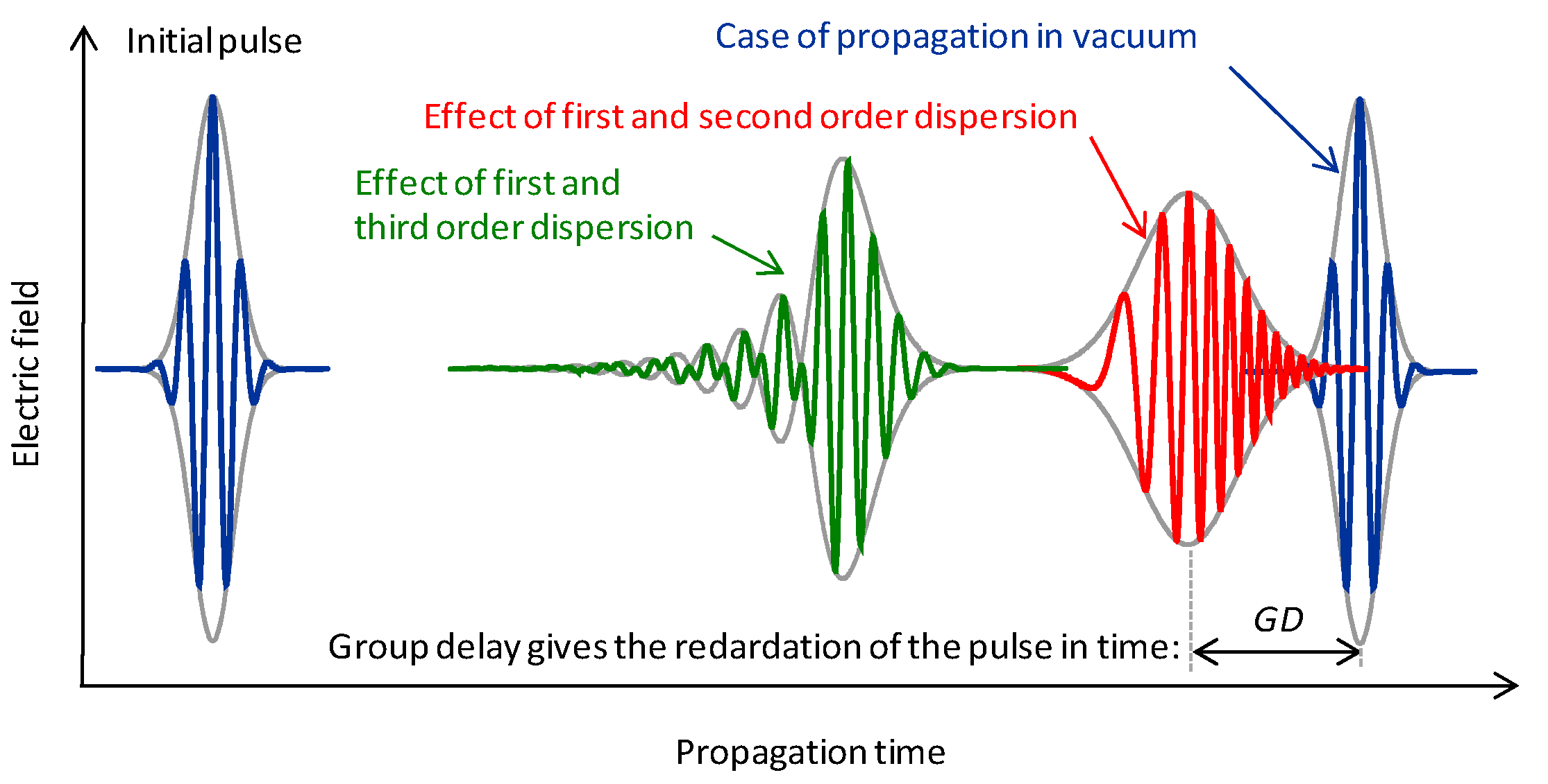
Figure 1 shows the effects of the first three derivatives on the carrier wave and the envelope. The shape of the pulse in the case of
TOD is calculated numerically.
Figure 1.
Schematic temporal effect of the first three phase derivatives.
Figure 1.
Schematic temporal effect of the first three phase derivatives.
For few-cycle pulses, the position of the carrier wave under the envelope plays a significant role since the outcome of many experiments could be drastically influenced if the electric field exceeds the ionization threshold by more or less one time during the course of a pulse relative to the previous ones. The quantity for the characterization of this property is the phase at
t –
GD = 0 (
i.e., at the peak of the pulse) and is the so-called
carrier-envelope phase (
CEP, see
Figure 2), which can be approximated by
Figure 2.
Definition of the carrier-envelope phase.
Figure 2.
Definition of the carrier-envelope phase.
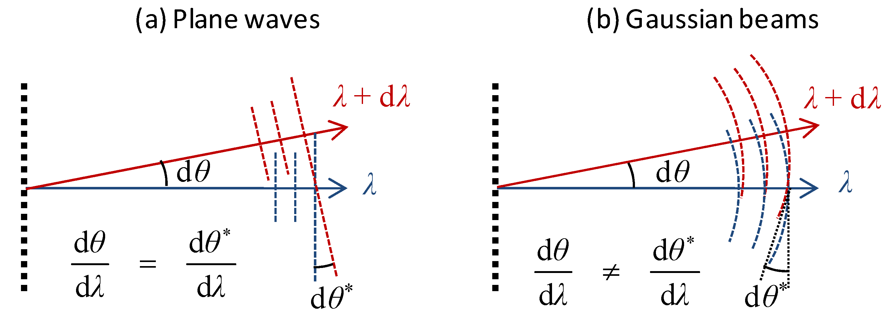
The different spectral components of an ultrafast laser pulse may propagate not only at different velocities but also into different directions. In this latter case, the propagation is affected by the angular dispersion. Such phenomenon takes place when e.g., a beam of ultrashort laser pulses refracts at the boundary between media with different dispersions, passes through a prism, or diffracts on a grating.
Angular dispersion can be defined in two ways. The most obvious one, based on geometrical optical considerations, is the wavelength dependence of the direction of propagation of the different spectral components, and is called
propagation direction angular dispersion, denoted by
γPD [
26]. The other definition originates from wave optics and hence addresses the wavelength dependence of the angle between the phase fronts; this approach results in the so-called
phase front angular dispersion,
γPF [
27]. Comparing the two definitions (
Figure 3), one can see that they are equivalent for plane waves, but different for spherical, hence the Gaussian beams [
28].
Figure 3.
Comparison of the two types of angular dispersion in the case of plane wave and Gaussian beam approximation.
Figure 3.
Comparison of the two types of angular dispersion in the case of plane wave and Gaussian beam approximation.
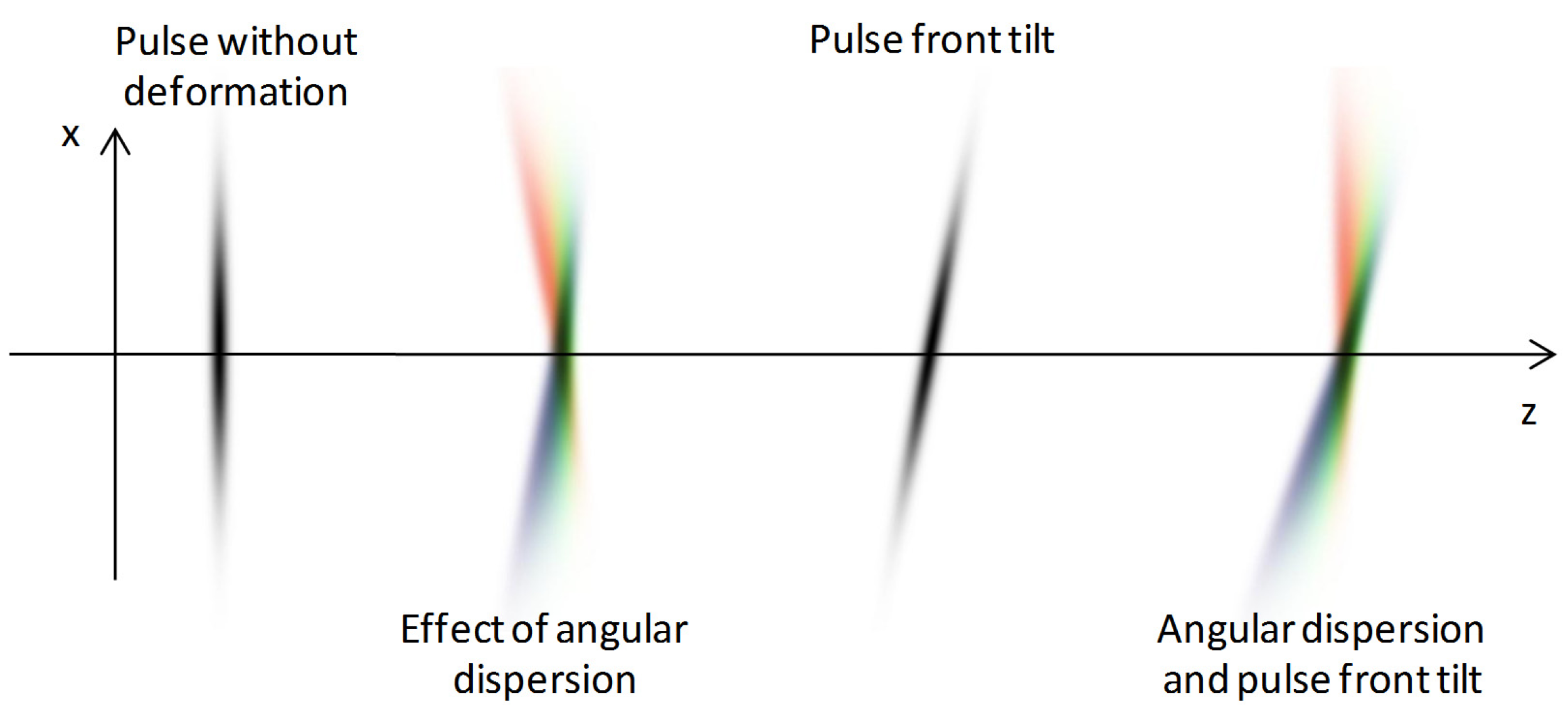
Figure 4 demonstrates the effect of angular dispersion on ultrashort laser pulses propagating in vacuum. The spectral components of the initial pulse are spatially and temporally overlapping, but their directions of propagation are slightly different due to the angular dispersion. In the case of plane waves propagating in vacuum (or in any isotropic media), the magnitude of angular dispersion remains constant; however, its effect on the pulse becomes more significant with increasing path length of the pulse travelling from the source of angular dispersion. Conversely, the magnitude of angular dispersion affecting Gaussian beams usually decreases during propagation [
28].
Figure 4.
Illustration of spatial effects of the angular dispersion and pulse front tilt.
Figure 4.
Illustration of spatial effects of the angular dispersion and pulse front tilt.
In
Figure 4, the spatial intensity distribution of the spectral components constituting the pulse is represented for different scenarios, after having propagated a certain distance of
z. If angular dispersion is present, with increasing distance measured from the middle of the pulse along the direction
x perpendicular to the direction of propagation, pulse length also increases and the spectrum becomes shifted at the same time. The pulse length in the center (at
x = 0) will also differ from the original pulse length, since the pulse will be affected by a phase modulation [
19] corresponding to the group delay dispersion
This can be converted easily into a stretch in pulse length based on Equation (12) [
29].
Angular dispersion is practically always accompanied by some pulse front tilt and spatial chirp, both demonstrated in
Figure 4. Pulse front tilt means a group delay along the cross-section of the beam, in the direction perpendicular to the propagation
z and with a magnitude of 2
πc∙
γPD/
ω0 per unit length along the cross sectional area [
19,
30,
31]. Spatial chirp involves a spatial anisotropy in the spectral content across the beam [
32]. This means that one part of the beam (the blue side of the pulse in
Figure 4) is shifted toward the shorter wavelengths, while the other part (the red side of the pulse) is shifted toward the longer wavelengths.
One can see easily that spatiotemporal pulse distortions usually arise simultaneously; moreover, they are coupled with each other. A general mathematical analysis of these coupling effects is discussed in Reference [
33].
3. Linear Optical Methods for Pulse Characterization
3.1. Historical Outlook
The nature of ultrashort pulses makes it more convenient to examine their properties in the spectral domain instead of the time domain, simply because detectors that are fast enough do not exist yet. However, steady or slowly changing patterns can be created by the means of interferometry. By its nature, it is extremely sensitive to the phase properties of short pulses, which is also very important to know in the temporal reconstruction process. Therefore, the possibility to involve interference methods for ultrafast pulse characterization becomes evident. When interference patterns are recorded in the time domain, multiple shots and pulse scanning are usually required. On the contrary, however, in the spectral domain, it is feasible to have single-shot measurement without moving parts. The spectral distribution of the pulse can be easily measured by spectrographs, and can be transformed to the time domain to calculate the transform-limited pulse duration. Last but not least, some of the special propagation issues may require the detection of the intensity distribution of the pulse in space. The technique called spectrally and spatially resolved interferometry (SSRI) fulfills all of these aspects. SSRI employs two beams forming an angle during propagation, and the interferometric pattern is established via spatially tilted phase fronts. Spectral resolution of the produced interference results in such an interferogram, on which the pattern of the interference fringes almost directly reveals the shape of the spectral phase difference function, and thus the magnitude of spectral phase difference can be obtained by visual analysis.
Methods using crossed-beam interferometry date back relatively early, well before the age of lasers. L. Puccianti published his first measurement results about the anomalous dispersion of oxy-hemoglobin [
34] in 1901. Eleven years later, D. Roschdestwensky used essentially the same technique to measure the oscillator strengths of atomic transitions in sodium vapor [
35]. In his experiments, he placed a test tube containing metal vapor into one arm of a Jamin– or Mach–Zehnder interferometer, and empty tube in the other in order to compensate the dispersion of the end-windows. Near the absorption lines, a hook-like interference pattern emerged, and a high-precision measurement could be obtained by reading off their spectral position. An analytical description of this hook method (
Hakenmethode) was presented by Marlow [
36]. After photo plates had been replaced by
CCD detectors allowing for a computerized analysis, H.J. Kim and B.W. James established a Fourier transform-based evaluation method that significantly improved the accuracy of the measurements [
37].
At present, the
SSRI method is preferable for investigating the ranges of normal dispersion rather than for anomalous dispersion. In early years, this method was used to determine the phase dispersion of metal layers [
38] and multilayered thin films [
39]. Later, researchers turned toward its ultrashort pulse-related utilization through high-precision measurement of the spectral phase shift of dispersion-compensating laser mirrors [
40,
41,
42,
43,
44]. The extended versions of
SSRI using arbitrary broadband light source (e.g., white light or ultrashort laser pulses) quickly became a widespread technique. In addition to further measurements on the phase shift of dispersion-compensating chirped mirrors [
45,
46],
SSRI was used among others for pump-and-probe experiments [
47], fine adjustment of the stretcher and compressor units of phase-modulated pulse amplifying systems [
48], characterization of laser pulses [
49,
50,
51], as well as the investigation of devices controlling the temporal shape of laser pulses [
52,
53]. Most recently, a high-power passive optical resonator was studied by this technique [
54]. In addition, a linear interferometric method has even been proposed for characterization of attosecond pulses [
55].
How these linear interferometric methods essentially work will be described in the next section, taking the general case of spectrally and spatially resolved interferometry.
3.2. Spectrally and Spatially Resolved Interferometry
The experimental implementation of
SSRI is based on the combination of a two-beam interferometer and a two-dimensional imaging spectrograph. For the sake of simplicity, a Mach–Zehnder interferometer is considered, illuminated by a broadband light source (
Figure 5).
The arm of the interferometer containing the dispersive object is called the sample arm; the other one is the reference arm. The spatial and spectral intensity distribution of the laser pulses travelling through the corresponding arms are denoted by IS(y,ω) and IR(y,ω), respectively. The pattern is finally detected by a spectrograph, which is equipped with a two-dimensional CCD detector. For the pulses propagating in the reference arm, the shape of the spectral phase function at the output generally is not influenced by the sample arm and remains unaltered; therefore, these pulses can be considered a reference for the measurement of the spectral phase change caused by the dispersive sample. However, a delay stage is inserted usually in the reference arm in order to adjust the timing of the reference pulses.
Figure 5.
Schematic experimental layout of the SSRI technique.
Figure 5.
Schematic experimental layout of the SSRI technique.
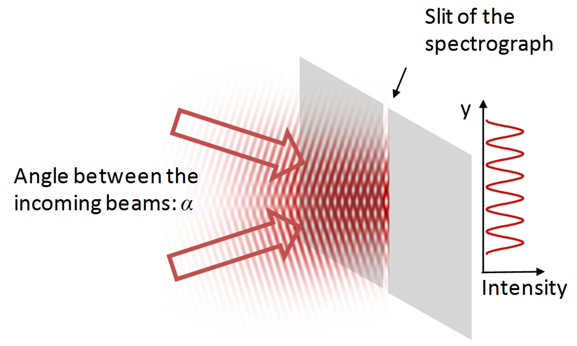
In order to establish a spatial resolution, the angle between the crossed beams must also be adjusted. The outcoupling mirrors of the individual arms are tilted vertically so that the beams cross each other at an angle
α, and overlap spatially along the vertically aligned slit. After the correct adjustment of the spatial and temporal overlapping of the pulses travelling through the sample arm, a vertically modulated interference pattern emerges on the spectrograph slit as illustrated in
Figure 6.
The interference pattern on the two-dimensional detector surface of the imaging spectrograph is described by
where the phase of the interferogram can be calculated as
Figure 6.
Formation of interference in the case of crossed monochromatic beams.
Figure 6.
Formation of interference in the case of crossed monochromatic beams.
In the formula above,
φS(
ω) and
φR(
ω) denote the spectral phase of the pulses arriving from the sample arm and the reference arm, respectively. These quantities are supposed to be independent of the spatial coordinate
y. The third term of Equation (17) describes a phase modulation in direction
y, caused by the crossed arrangement of the beams, assuming that
α is small (see
Figure 6). Here
y0 denotes a reference point, where the phase difference arising from the tilted phase fronts is zero. At this height, the total group delay at the central frequency of
ω0 is exactly the same for the pulses travelling along the two different pathways when an empty interferometer is considered. If the group delay in any of the arms changes (e.g., the length of the reference arm changes through the operation of the delaying unit, or extra material is inserted into the sample arm), the equal
GD level will be shifted along the
y axis from the position of
y0.
The spectral phase shift in the arms of the interferometer can be approximated by Taylor expansion, similarly to Equation (5). If
LS and
LR distances are supposed to be travelled by the laser pulses in the arms filled by a medium (usually air) having an index of refraction
nmed, then their contributions to the total spectral phase shifts can be written as
where
X can be replaced by either
S or
R, depending on whether the sample arm or the reference arm is considered. Beside these factors, a further phase shift must be considered, induced by certain optical elements such as beam splitters, output couplers, filters, dielectric and chirped mirrors. Those physical quantities which summarize their effects will be denoted by a superscript index “
opt”. Since phase derivatives are additive quantities according to the theory of laser pulse propagation discussed before [
19] (this can easily be shown if their linear dependence of
z is considered), the total phase derivatives of the sample arm are
while that of the reference arm are
A precondition of interference is that the components with identical frequency should coincide within the coherence time and the coherence length. Interference can emerge not only between such laser pulses, which were generated at the same time. Those interferometers which establish interference between consecutive laser pulses at their outputs are called asymmetric interferometers. In this case, the optical path difference of the arms must equal to the multiple of distance between subsequent pulses of the train. Based on Equation (10), pulses propagating in different pathways will overlap each other in time if the difference of the total group delays between the arms and the delay corresponding to
m periods of the temporal separation between the pulses (the latter originates from the asymmetry of the interferometer) are together within the coherence time
tcoh,
i.e.In the frames of the spectral resolution of ultrashort laser pulses, the meaning of coherence time slightly differs from its common definition, since here the coherence of the individual modes of the frequency comb must be considered. This falls in the picosecond range, taking into consideration that the line width of a mode is approx. 150 Hz [
56]. In this case, the observation of interference is (beside the noise resulted from the mechanical vibrations of the interferometer) only limited by the resolution of the spectrograph, which may correspond to several millimeters in terms of the difference between the arms.
Figure 7.
Simulated SSRI interferogram with arms of equal dispersions.
Figure 7.
Simulated SSRI interferogram with arms of equal dispersions.
Figure 7 demonstrates a typical interference pattern resulted in a
SSRI, when the dispersion in the arms is identical. The interferogram presented here is centered along the vertical axis to the position of
y0, and the interference fringe corresponding to this height is set to be horizontal. In the interferogram, interference fringes diverge in a fan-shaped manner from left to right toward increasing frequencies, thereby increasing also the periodicity of the
y-directed modulation.
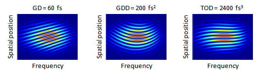
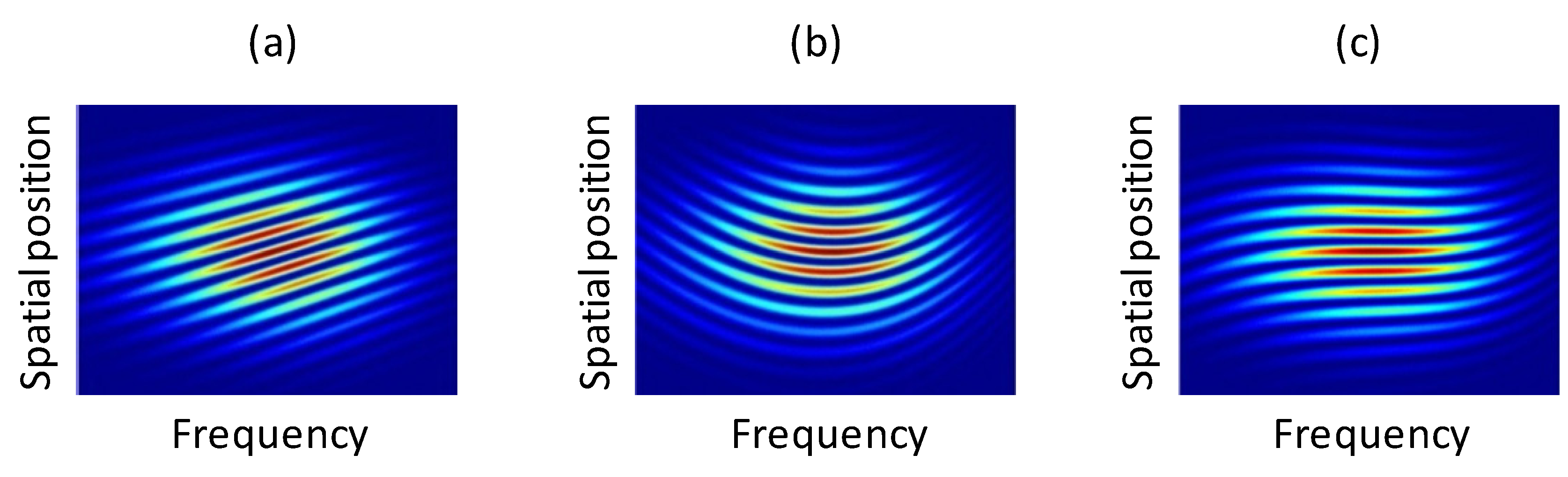
Figure 8.
Demonstration of separated effect of phase derivates on simulated interferograms. The values of the applied phase derivates are GD = 60 fs (a), GDD = 200 fs2 (b) and TOD = 2400 fs3 (c), respectively.
Figure 8.
Demonstration of separated effect of phase derivates on simulated interferograms. The values of the applied phase derivates are GD = 60 fs (a), GDD = 200 fs2 (b) and TOD = 2400 fs3 (c), respectively.
With increasing distance measured from the position
y0 along the spatial axis
y, the slope of the interference fringes increases in absolute value, which can be explained by the group delay between the phase fronts corresponding to the position
y. If the spectral phase difference between the two arms is not zero, then the pattern of the interferogram exactly follows the shape of the spectral phase difference function between the sample arm and the reference arm, apart from the extra group delay caused by the distance measured from the position
y0.
Figure 8 demonstrates how the effect of the phase derivatives of different orders are reflected in the interferograms.
3.3. Pulse Measurement
As it may become obvious from the preceding sections,
SSRI offers a fast, simple and robust technique to measure the relative spectral phase of an unknown pulse to a well-described one. That is, unlike other pulse characterization techniques based on the (nonlinear) interferometry
SPIDER [
18,
21] and similar solutions,
SSRI is a linear, but not a self-referencing method [
49]. Hence, the parameters of the reference pulse have to be well known at a certain point of the laser system (e.g., at the output of the oscillator, or measured by a different technique, which provides absolute measurements). Let us suppose that the phase derivates between the reference point and the input of the interferometer change by
during the free-space propagation of the geometrical length of
LF and passing through certain optical elements with well-known dispersion (
![Applsci 03 00515 i045]()
). If the absolute phase derivates at the reference point are
GDRP,
GDDRP and
TODRP, the pulses of the sample arm at the output of the interferometer are characterized by
where Δ
GD, Δ
GDD and Δ
TOD are measured from the recorded interferograms. This process gives a simple method to determine absolute pulse parameters at basically any point of the system.
Please note that this is basically a single-shot, linear method which describes the absolute spectrum and the relative spectral phase of the pulse to be characterized, so that the relative temporal shape can be calculated to great accuracy. Linear interferometric methods can be utilized in most of the practical applications like spectroscopy, linear and nonlinear dispersion measurements, time-resolved studies, as well as compressor alignment and beam monitoring along high intensity laser systems. On the one hand, these methods provide the experimentalists with more accurate information than the nonlinear measurements methods, which offer an absolute temporal shape, but with a factor of 2–5 higher error than the linear methods. On the other hand, the linear methods would never be able to provide the absolute pulse duration on their own, since the first-order auto- (and cross-) correlation function to be determined by linear interferometry offers coherence information of the interacting pulses only [
19].
3.4. Dispersion Measurement of Optical Elements
Although the
SSRI measures only the relative spectral phase of a light pulse, even this can be used for
absolute measurement of dispersion of any optical element. The scheme is simple: let us measure the relative spectral phase of a light pulse to a reference pulse before and after the optical element. The difference of spectral phases arises purely from the dispersion of the optical element. In detail, as the first step of the measurement, differences of phase derivatives are measured in case of the empty interferometer, so the phase derivatives of the arms are revealed as:
After an identical group delay has been adjusted, the left side of Equation (24) equals to zero, therefore
can be written, where
m equals zero if the same pulses interfere at the output, which were split at the input of the interferometer.
In the second step, the sample having a geometrical length of
Lsample is inserted in the sample arm of the empty interferometer. This leads to the fact that Equations (32)–(35) will be applied with the following modifications: on one hand, the laser pulses will travel in the sample arm a length shorter by
Lsample compared to the empty interferometer, thus
and on the other hand, the length of the reference arm must be modified by Δ
LR to compensate the group delays, thereby
After this adjustment, the equation
GDS –
GDR =
m’T can be used, where
m’ is an integer as well, though not necessarily the same as
m. For the group delay of the sample
can be deducted. The group delay dispersion is given by
where Δ
GDD(0) and Δ
GDD are obtained from the evaluation of the interferograms captured during the two measurements. Similarly, third-order dispersion can be acquired from
Depending on the nature of the sample, further measurements are also possible if the spectral phase shift of the sample can be tuned in such a way that neither the sample length nor the phase derivatives of the other components of the interferometer change (for example, changing the temperature of an optical element, the concentration of a solution, or the pressure of a gas). Besides such tuning of a state variable of the sample, equal group delays should be adjusted before each measurement if necessary, and the differences of the phase derivatives will finally be determined. If the dispersions of all the other elements within the system remain constant during the series of measurement, the correlation between the object’s variable quantity and the phase derivatives of the sample’s material can be represented by a fitted function.
After the first experimental demonstration of pulse measurement by the
SSRI [
49], its precision and reliability were investigated in an extensive study in Reference [
57]. Simulations showed that one of the most dominant sources of inaccuracy originates from the noise of the spectrograph’s detector. Cooled
CCD can reach such signal-to-noise levels, where
SSRI is capable to provide 0.02 fs
2 and 0.7 fs
3 precisions in
GDD and
TOD, respectively. Without cooling, 0.1 fs
2 and 2 fs
3 can be considered typical values. The effect of bandwidth, fringe visibility and density, spherical phase fronts (based on Gaussian beam approximation), optical path fluctuations and intensity irregularities were also examined separately in Reference [
57].
When the determination of specific phase derivatives are the aim of an experiment, the precision is affected by the measurement accuracy of the geometrical length of the object. Depending on the length of the object, e.g., interferometric length measurement methods (for under mm scale), micrometer screw gauge (for mm scale), vernier caliper (for mm and cm scale) or laser rangefinder (for cm and m scale) are to be used. Hence, the geometrical length can be determined with an accuracy higher than 0.1 percent, which is at least one order of magnitude better than the accuracy of the phase derivatives.
A modified version of crossed-beam interferometry-based techniques combined with
SPIDER and
FROG methods resulted in the so-called spatially encoded arrangement for temporal analysis by dispersing a pair of light
E-fields,
SEA-TADPOLE [
51]. This method reveals interference patterns almost identical with that of the
SSRI methods, although the experimental implementations of the two methods are different. The implementation of spatial encoding significantly improved the accuracy of the former
SPIDER and
FROG methods [
58,
59,
60,
61,
62].
3.5. Spectrally Resolved Interferometry
One of the most common methods used for the measurement of spectral phase shift is the so-called spectrally resolved interferometry,
SRI [
63,
64,
65,
66,
67,
68,
69,
70,
71,
72], which can be interpreted as a special case of
SSRI when
α = 0. The beams here leave the Michelson or Mach‑Zehnder interferometer in a collinear manner, and an interference is established due to the temporal delay
t* within the time scale of the coherence time, kept to be constant between the beams. The beams are directed in a spectrograph and reveal a modulated spectrum as represented in
Figure 9a. The larger
t* delay is set the narrower is the period of the modulation. Since in most cases spatial modulation is not present along the slit, a spectrograph with array detector is sufficient.
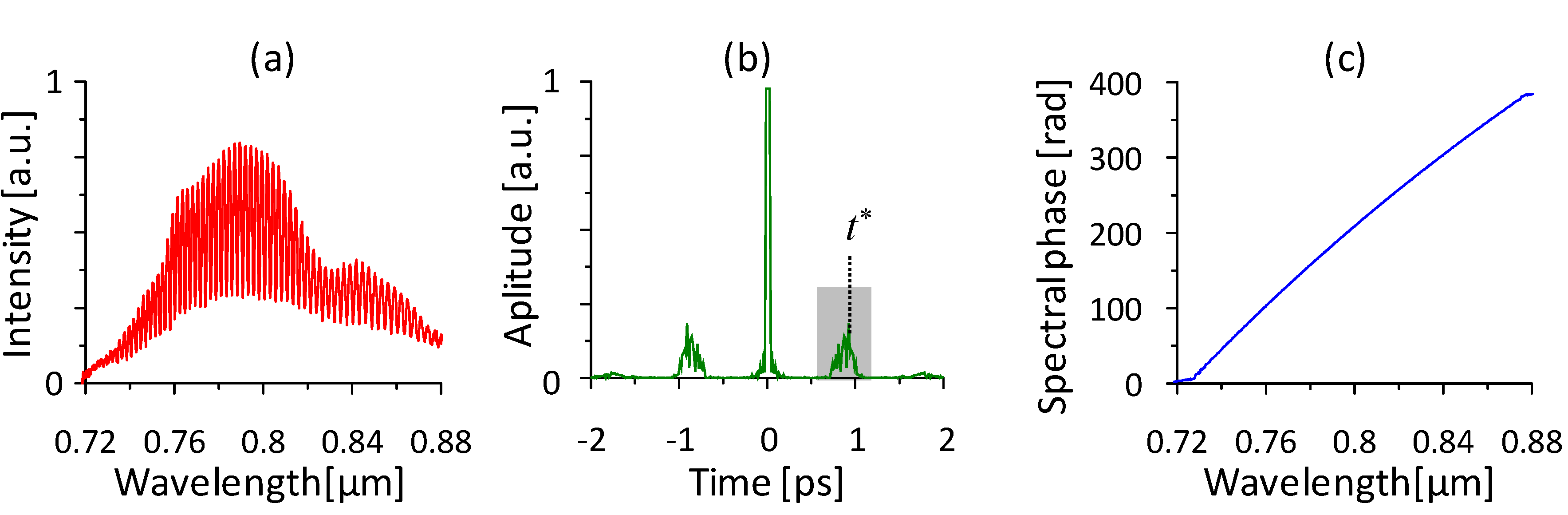
One of the most widely used Fourier transform-based evaluation methods of
SRI interferograms was developed by Lepetit
et al. [
64]. According to his method, the measured spectral interferogram (
Figure 9a) is first inverse Fourier-transformed, and then a filter is applied on it at the time difference corresponding to the time interval between the pulses,
t*, using a window function having optimal width (
Figure 9b). In the final step, the filtered signal is transformed back into the spectral domain. The angle of the complex values of this spectrum reveals the spectral phase difference of the pulses (
Figure 9c). The slope of the phase at
ω0 corresponds to
ω0·
t*, and the phase derivatives of higher orders can also be determined by a polynomial fitting.
This method can be used with broadband laser pulses as well as with continuously operating white light sources, since the only precondition of the measurement is that the spectral bandwidth of the light source should be broad enough.
SRI is thereby often used to determine the dispersion of optical material, using an interferometer illuminated by continuously operating white-light lamps [
43,
44,
73,
74].
Figure 9.
Steps of the spectral phase calculation by Fourier-transform SRI. The recorded interferogram (a) is inverse Fourier-transformed to time domain, and filtered (b). Finally, the remainder is transformed back to spectral domain. The complex angle corresponds to the spectral phase difference between the arms of the interferometer (c).
When overwhelming difference in dispersion of the sample and reference arms is present,
SSRI and
SRI might be able to resolve the interference pattern only on a small wavelength range of spectrum. Stationary phase point method,
SPP [
75,
76] is an implementation of
SRI (
i.e.,
α = 0 is still a necessary condition), which can be applied in this case. The plane-wave approximation can no longer be applied because the different curvatures of the phase fronts play an important role in the position-dependence of the phase difference occurring between the pulses that meet on the detector surface.
SPP method is based on the determination of the spectral position of the stationary phase point as a function of the delay between the sample ad the reference pulse. This technique is particularly useful when one wants to compare stretched pulses of a
CPA system with nearly transform-limited seed pulses from the oscillator [
48]. It has been also proved to be useful during the measurements of the dispersion of optical fibers [
77,
78,
79].
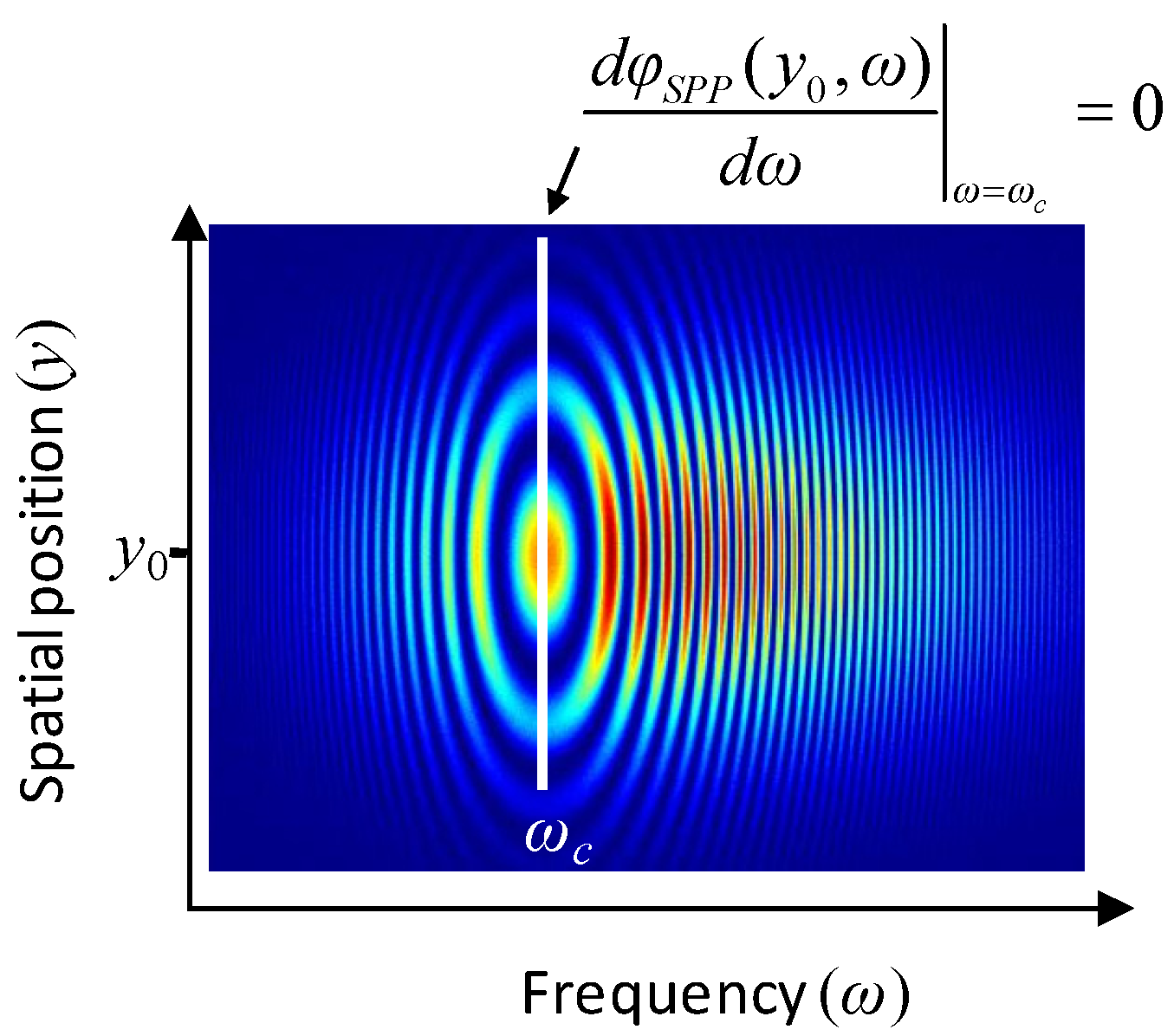
Figure 10.
A typical example of spectrally and spatially resolved interferograms with the stationary phase point.
Figure 10.
A typical example of spectrally and spatially resolved interferograms with the stationary phase point.
Let us suppose that the two beams are coaxial, and they reach the detector at the position
y0. The stationary phase point is located at the central frequency
ω0, if the group delays of the arms are carefully aligned to satisfy the condition in Equation (30). In this case, the temporal delay
t* is zero. When one introduces the delay
t* of the pulses of the sample arm, the stationary phase point will be shifted along the
ω-axis. We can neglect the dispersion of the medium surrounded by the interferometer (usually air), since the dispersion difference in the arms is greater by several order of magnitudes. The spectral phase difference can be written as a modified form of Equation (10), namely
The first derivative by
ω of Equation (41) gives
if
ω* is the frequency where the stationary phase point is observed. Eventually, scanning through the spectrum of the pulse, the difference of the group delay between the arms can be measured with respect to the
ω*, since
t* can be calculated easily from length position of the precision translator. The first and second order coefficients of polynomial fitted on the
t*(
ω*) relationship will provide the
GDD and the
TOD difference between the arms, respectively. It can be seen that the larger the
GDD to be measured, the more accurate the
SPP method; therefore, it is especially appropriate for the measurement of stretched pulses. However with decreasing the relative
GDD, the width of the interference fringes (
i.e., their extension along the
ω-axis) increases, and the determination of the position of the stationary phase point becomes unreliable. In such a case, the position can only be obtained by fitting a phase modulated cosine function. Although the
SPP method can improve the accuracy of dispersion measurements, no additional information is provided compared to the dispersion calculated from the parameters of the phase-modulated cosine function fitted on the data at one single delay [
80].
It is worth mentioning that the elliptical nature of the two-dimensional fringes (as illustrated in
Figure 10) was observed as early as in 1927 for glass plates used as samples [
81].
A spectrograph equipped with two-dimensional detector for this measurement in order to ensure collinearity has been suggested. However, the position of the stationary phase point can be determined even if only a one-dimensional detector (e.g., a diode array) is available, positioned parallel to the wavelength axis. Stationary phase point method does not exploit the information about the dispersion of the sample encoded in the two-dimensional structure of the fringes.
The accuracy of measurement by
SRI method was thoroughly examined by Dorrer
et al. [
66,
67,
68]. Among other error sources, spectral calibration issues, detector response inaccuracies, resolution and sampling problems were investigated. Experimental demonstrations showed about 1% relative error in the determination of
GDD, which is a little bit worse comparing to
SSRI [
57].
3.6. Evaluation of Interferograms
One of the simplest methods of interferogram evaluation is based on cosine function fitting. This method requires the intensity distribution of the individual arms. Substituting these values into Equation (16), a normalized intensity
can be revealed. Then
y coordinates should be limited to a range where noise is supposed to be negligible, in order to avoid misleading phase information. After normalization,
Figure 11 shows the basic steps of the evaluation of interferograms. In step 1, a function of
f(
x) = cos(
a·
x +
b) form is to be fitted with the least-square method on the
ith column, corresponding to the angular frequency
ωi. This procedure results in parameters
ai and
bi. If the regression procedure is applied to only a short range (e.g., one and a half cycles, marked with red curve in the plot for step 1 in
Figure 11.) at one time, the residual irregularities of the normalized interferogram have less influence on the extracted phase and the fitting information can be retrieved pixel-by-pixel. This fitting routine needs to be carried out on each column of the interferogram. In step 2, a phase surface can be constructed from the regression results.
Figure 11.
Steps of the phase extraction from the interferograms.
Figure 11.
Steps of the phase extraction from the interferograms.
From the aspect of the spectral phase, the values of bi parameters play an important role. The cosine fitting causes an ambiguity, namely that beside bi, every bi + q·2π value can be the solution of the fitting, where q is an arbitrary integer. Therefore, when connecting these bi values along the phase jumps of q·2π, the resulting value will only differ from the spectral phase with the whole multiples of 2π. This constant difference, however, does not affect the values of the phase derivatives, so they can be obtained by fitting a proper (usually third-order) polynomial function.
4. Multiple-Beam Interferometer for CEP Drift Measurement
The influence of the
CEP on the outcome of experiments increases dramatically with decreasing the duration of the pulses driving the interaction below a few optical cycles [
82]. The generation of high harmonics [
83,
84,
85] and attosecond pulses [
86,
87,
88], as well as frequency comb-based metrology techniques [
89] demand precise detection and subsequent low-jitter stabilization of
CEP [
90]. Nowadays,
CEP stabilization is well-established for Ti:sapphire lasers by the means of
f-to-2
f and
0-to-
f interferometry [
91,
92]. Recent developments suppressed the CEP noise of the few cycle pulses in the visible- near infrared spectral range to a previously unexpected level of a few tens of mrad [
93,
94]. Unfortunately, a wide range of lasers cannot satisfy the necessary conditions for such nonlinear interferometries [
92]
i.e., octave-spanning spectrum or enough power for frequency doubling. It is possible to overcome the condition of broad spectrum by the generation of white light continuum of the laser pulse to be measured, but it requires a complex experimental setup with multiple nonlinear conversions [
95].
Similarly to the dispersion coefficients, the
relative CEP between two interfering pulses can be also measured by
SSRI and
SRI. The difference in
CEP can be calculated from Equation (13), where
φ(
ω0) and the
GD are derived from spectral phase of the recorded interferogram. It can be used effectively to observe a phenomenon which introduces variation to the
CEP of the pulses only in the sample arm, when certain properties of the sample object are modified. Another useful application of these methods is using them to determine the jitter of
CEP between the arms. For instance, from the blurriness of the interference pattern, one can deduct that how stable the fringe position and density during the integration time of the detector is [
96].
Not only the relative
CEP of a pulse, but also the
CEP drift of a pulse train, can be determined. The most advanced device relies solely on a multiple-beam interferometer (
MBI) and a spectrograph [
97,
98]. The advantage of using spectrally resolved interferometry is that besides properties of the detector, the system is practically free of wavelength conditions, including the bandwidth, the spectral range or the central wavelength. This technique offers not only the measurement of the pulse-to-pulse
CEP drift, but also seems to be fast enough to apply feedback to lasers with prohibitively low pulse energy for regular
CEP stabilization schemes. Moreover, this scheme allows simultaneous monitoring of intracavity refraction and linear dispersion for a virtually unlimited range of mode-locked lasers, including monolithic designs where such insight is otherwise difficult to obtain [
54].
Figure 12.
Schematic layout for the linear detection of the CEP drift (a). The variation of the actively stabilized path length provides the accuracy of the CEP measurement at 800 nm (b).
Figure 12.
Schematic layout for the linear detection of the CEP drift (a). The variation of the actively stabilized path length provides the accuracy of the CEP measurement at 800 nm (b).
Instead of using Michelson and Mach–Zehnder interferometers, a resonant ring layout was implemented to keep information of the pulse phase for several round trips (see
Figure 12a). After a part of the initial pulse makes one round trip in the
MBI, at the output––if the ring length is carefully aligned––it will interfere with the next pulse of the train. The rest of the pulse before the initial one is still in the system, and it also contributes to the interference, although with a lower intensity. This effect is similar to the principle of the Fabry–Perot interferometer, and it will result in a weighted averaging for many subsequent pulses. In the spectral domain, spectral interference fringes will appear, very similarly to the case of
SRI.
If the
MBI is free from second and higher-order dispersion, the fringe pattern could be described simply by two parameters: fringe position (
i.e.,
φ(
ω0)) and spacing (
i.e.,
GD). This could be important in those cases where fast detection and response is required, most notably, for
CEP stabilization. Practically, the spacing of the spectral fringes, or more precisely their deviation from equidistance, is affected by the
GDD of the multilayer mirrors [
99], the ambient air of the interferometer [
100] and beam splitters forming the cavity. Small residual
GDD contributions can be removed from the phase extraction by suitable calibration as long as they are static. Therefore, linear interference in a single ring resonator suffices, in principle, to completely characterize the
CEP drift of a pulse train. All required information is readily retrieved from the measured spectral interference pattern via Fourier processing [
64]. Due to the independent thermal drift of the laser oscillator and the
MBI, at least the optical path length of
MBI has to be carefully stabilized. In the developed device [
101], it is achieved with a frequency-stabilized He–Ne laser. The half of
cw beam follows the exact same path like the ultrashort pulses (but in the opposite direction) and interferes with the other half of the beam. The interference fringes are deflected directly to the
CCD detector. The recording and fast evaluation of the pattern drives the piezo translator to compensate for the eventual change of the optical path. The recorded path length variation is showed in Fig 12.b. For the sake of an easy comparison with
CEP noise of the ultrashort pulses, the actual length values are converted into optical phase noise at 800 nm, and over an 8-h period, a noise of 68 mrad
RMS was measured. This type of stabilization can dramatically decrease the noise in
CEP drift detection. A comparative study showed exceptional agreement with the results obtained from the
f-to-2
f technique, while demonstrated 120 mrad
RMS noise of the
CEP drift provided by the
MBI method [
98].
The significance of this technique was emphasized by the
CEP drift measurement of a picosecond laser with less than 0.2 nm bandwidth [
102]. An ultrahigh finesse, long Fabry–Perot cavity, designed for Compton backscattering applications, exhibited severe sensitivity to the instabilities of the frequency comb. Its error signal was related to the carrier-envelope offset frequency, the equivalent quantity for
CEP drift in the frequency domain. The
MBI was equipped with an ultrahigh resolution spectrograph, and recorded the
CEP drift simultaneously. When the repetition rate of the oscillator was manually varied, the error signal for the Fabry–Perot cavity and the
CEP drift measured by the
MBI showed very good agreement, which is an undeniable proof of the capability of the
MBI method to detect the
CEP drift independently from the spectral bandwidth of the laser.
5. Methods for Angular Dispersion Detection
5.1. Measurement of Propagation Direction Angular Dispersion
The characterization of the angular dispersion of ultrashort laser pulses is inevitable when complete spatiotemporal compression of the pulses is necessary. When the angular dispersion is not compensated carefully, it can lead to an unexpected decrement in the peak intensity. At the same time, spectral components may also be separated spatially, thereby inducing a so-called spatial chirp, which involves an asymmetry of the spectral content in the beam profile. A direct consequence of this spatial chirp is the tilt of the phase front, which raises some further unwanted increase in the pulse duration. Elimination of angular dispersion (i.e., the divergence of the spectral components) does not necessarily remove the spatial chirp, since the spectral components may still propagate along distinct parallel axes, even if they travel in the same direction.
A simple and direct method to measure of propagation direction angular direction is based on spectrally and spatially recorded intensity distribution of the focused spot of the beam. The layout of the technique is shown in
Figure 13.
Figure 13.
Schematic diagram for measuring the propagation direction angular dispersion.
Figure 13.
Schematic diagram for measuring the propagation direction angular dispersion.
An achromatic lens or spherical mirror is used to focus the beam on the slit of the spectrograph. In case of angular dispersion, spectral components have different propagation directions, therefore, in the focal plane, also a different spatial position. This position y is related to relative angle of the propagation direction of an actual spectral component, whereby the component’s frequency needs to be determined. This can be done with a spectrograph, which provides a spectrally resolved intensity distribution on its detector and eventually leads to a tilted and elongated spot on the image. The angle of the tilt corresponds directly to the propagation direction angular dispersion.
Unfortunately, this method can only detect the angular dispersion along the cross-section of the beam, which is defined by the slit of the spectrograph. In most cases, it is highly desired to ensure that the beam is free of angular dispersion in both horizontal and vertical direction. It can be executed only when the beam or the spectrograph is rotated by 90°. For this purpose, it is most convenient to use a mechanical beam rotator, which is practically a twistable periscope, but does not alternate the direction of the beam when it is passing through.
Since this method is limited to measure along one spatial dimension only, at least two subsequent measurements required for complete beam profile characterization. This leads to a lengthy and iterative alignment of the stretcher-compressor stages of the
CPA system. Concerning the precision, it is typically sensitive for the pulse bandwidth and the focal length of the focusing element (
i.e., the sharpness of the elongated spots). During alignment of compressor systems, an accuracy of 0.1 μrad/nm was demonstrated [
103].
5.2. Two-Dimensional Detection Method for Propagation Direction Angular Dispersion
When a broadband light beam is affected by angular dispersion, its spectral components will propagate in various directions. If the beam is focused directly on the sensor chip of a two-dimensional detector by an achromatic imaging element, a relatively elongated spot will appear in the image compared to a beam without the effect of dispersion. The intensity distribution of this elongated spot is in direct correlation with the spectral angular deviation. However, the spot itself is not suitable for accurate measurements. On one hand, chromatic aberration of the spot must be separated from optical aberrations of different nature. On the other hand, this elongated spot contains no information on the spectral calibration required for the measurement, i.e., different parts of the spot cannot be matched with the frequency of the corresponding spectral components. Both problems can be eliminated with the purposive spectral modulation and calibration of the broadband beam.
A method for single-shot, two-dimensional measurement of propagation direction angular dispersion of broadband light sources (e.g., ultrashort laser beams) was introduced recently. In this case, spectral calibration is achieved by spectrally filtering the beam in order to create well-separated peaks in the spectrum. Since these components are still overlapping spatially, we use an achromatic lens to image them onto a two-dimensional detector. In this way, the spectrally separated components of an angularly dispersed beam will appear as dissociated spots on the surface of the detector according to the orientation of the angular dispersion.
The role of the spectral filter can be filled with various, either passive or active solutions. For example, multiple bandpass interference filters or wavelength-selective reflectors can be used for this purpose. Another very simple idea is to block parts of the spectrally resolved beam in the stretcher; although it might be not suitable, if the stretcher itself is the object of examination. Acousto-optical programmable modulators can be used also to create an arbitrarily modified spectrum. A less expensive solution to create separated spectral peaks is the use of a Fabry–Perot interferometer (
FPI) [
104] with either adjustable or fixed baselength, which allows high spectral purity when one is using high-reflection mirrors. When it is equipped with a precision translator, the wavelength spacing of the transmitted spectrum can be controlled easily through its baselength. This feature makes the
FPI the optimal choice as the spectral filtering device.
Figure 14.
Typical layout for simple, two-dimensional detection of propagation dispersion angular dispersion (a). If the original beam is not angularly dispersed enough to separate the peaks, an additional grating or prism can be inserted to have a well-known constant bias in the angular dispersion (b). On the right side, a sample image is shown (c).
The scheme of the technique can be seen in
Figure 14a, where a
FPI is pictured as a spectral filter. A broadband beam with unknown angular dispersion is propagating through the partially reflecting mirrors of the
FPI, where the spectrum of the beam becomes modulated, and thus well defined, sharp spectral peaks appear. The transmitted parts of the spectrum preserve their original propagation directions, which––in case of angular dispersion––can be different for each spectral component. However, the spatial distributions of these spectrally separated beams are still overlapping. For this reason, an achromatic lens is positioned after the
FPI to image the beams onto the chip of a two-dimensional detector.
When the beam has weak angular dispersion only, it is possible that the spectral spots cannot be separated effectively with the base length modulation of the
FPI. In these cases, a grating or prism with very well-known and calibrated angular dispersion can be inserted between the
FPI and the achromatic lens (see
Figure 14b). It provides an additional constant bias in the angular dispersion only, but with the spots very well separated, it increases the precision of the extraction of the spot coordinates, and by that, the precision of the measurement.
Experimental verification with different prisms showed that the precision does not decrease significantly compared to the one-dimensional method, as standard deviation from the expected values was 0.15 μrad/nm [
104].
5.3. Phase Front Angular Dispersion––An Absolute Measurement with SSRI
The
SSRI technique can be applied also for the determination of either the
relative (
i.e., occurring between the arms) or the
absolute phase front angular dispersion
γPF along the direction of the slit of the spectrograph. Keeping in mind that when reflected on a mirror, angular dispersion changes sign along the plane of reflection, the method can be modified accordingly. When a Mach–Zehnder interferometer is used with the same number of reflections in the arms (or their difference is an even number), the angular dispersion of an object inserted in the sample arm can be measured as the difference in angular dispersion of the interfering pulses. For the measurement of the
absolute angular dispersion, an
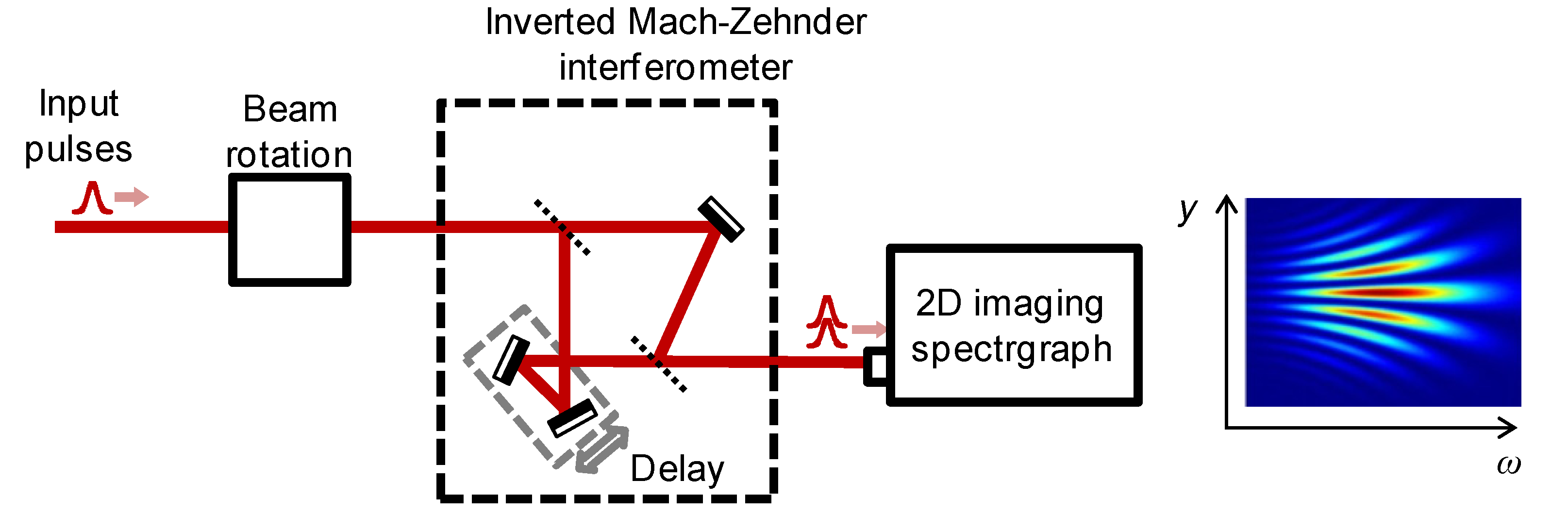
empty Mach–Zehnder interferometer has to be altered so that the difference between the numbers of reflections from optical surfaces in the two arms is an odd number (e.g., one arm should contain an additional mirror). Therefore, at the output of the interferometer, the pulse will establish interference with its replica, mirrored to the direction of the propagation. The magnitude of the angular dispersion will be unaffected by this reflection; however, its direction will be inverted. This implementation of the interferometer is called
inverted Mach-Zehnder interferometer [
105,
106]. The accordingly modified scheme is shown on
Figure 15.
Figure 15.
Experimental set-up of the interferometric detection of phase front angular dispersion with an inverted Mach–Zehnder interferometer.
Figure 15.
Experimental set-up of the interferometric detection of phase front angular dispersion with an inverted Mach–Zehnder interferometer.
The angle between the phase fronts will then be measured by spectrally and spatially resolved interferometry, and will depend on the wavelength due to the angular dispersion. If a small angle is adjusted between the beams in the direction of polarization, then this (wavelength-independent) angle will also occur between the phase fronts, and thereby the interference pattern will be modulated in the direction of polarization. The frequency of this modulation is directly proportional to the angle and to the frequency of the light. The manually adjusted angle between the beams can be measured as the function of the wavelength by a two-dimensional imaging spectrograph having a slit oriented in the direction of polarization. The derivative of the measured angle with respect to the wavelength results in a value twice the phase front angular dispersion occurring in the direction of polarization.
The angle between the phase fronts as defined by Equation (17) will depend on the wavelength. Using the parameters
ai of the cosine fit outlined earlier, α values can easily be obtained for each wavelength. Phase front angular dispersion reveals then as follows:
An inappropriate adjustment of the optical elements in a CPA system may cause an angular dispersion not only in the horizontal, but also in the vertical plane, therefore beam rotational stage is required here as well.
Accuracy of the phase front angular dispersion depends on the detector noise similarly as it was shown in the case of
SSRI [
57], since the phase extraction process is the very same in both cases. Experimental studies demonstrated 0.2 μrad/nm precision [
53,
106].
Spatial invertion of the beam profile can be effectively used in nonlinear autocorrelators as well. Since no spectral dimension is needed during the evaluation, both spatial directions can be inverted, hence pulse front tilt can be detected in 2D in a single-shot measurement [
107]. The accuracy of the phase front angular dispesion is similar to the linear method presented above; however, in case of Gaussian beams, it might be complicated to determine the phase front angular dispersion from the measured pulse front tilt [
108].


 ). If the absolute phase derivates at the reference point are GDRP, GDDRP and TODRP, the pulses of the sample arm at the output of the interferometer are characterized by


