Quantum Wind Driven Optimization for Unmanned Combat Air Vehicle Path Planning

Abstract

Unmanned combat air vehicle (UCAV) path planning aims to calculate the optimal or suboptimal flight path considering the different threats and constraints under the complex battlefield environment. This flight path can help the UCAV avoid enemy threats and improve the efficiency of the investigation. This paper presents a new quantum wind driven optimization (QWDO) for the path planning of UCAV. QWDO algorithm uses quantum rotation gate strategy on population evolution and the quantum non-gate strategy to realize the individual variation of population. These operations improve the diversity of population and avoid premature convergence. This paper tests this optimization in two instances. The experimental results show that the proposed algorithm is feasible in these two cases. Compared to quantum bat algorithm (QBA), quantum particle swarm optimization (QPSO), wind driven optimization (WDO), bat algorithm (BA), particle swarm optimization (PSO), and differential evolution (DE), the QWDO algorithm exhibited better performance. The simulation results demonstrate that the QWDO algorithm is an effective and feasible method for solving UCAV path planning.

1. Introduction

In recent years, with the rapid development of science and technology, modern battlefield military equipment has shown a clear trend toward unmanned operation. As an important means of airborne reconnaissance, surveillance and combat, the aircraft is increasingly a primary concerned of militaries around the world. However, with the increasing complexity of the modern battlefield environment and the continuous expansion of the scope of operation, UCAV not only need to avoid or reduce the probability of detection, but also avoid many adverse factors that may affect the flight in no-fly zones and barrier regions, which have brought serious challenges to the implementation of aerial reconnaissance, surveillance, combat and other missions to the UCAV. Therefore, in order to improve the operational efficiency and the survival probability, path planning must take into account the requirements of the task, the threat distribution, the fuel restriction and other constraints, when producing a global optimal or sub-optimal route that can effectively avoid the threat of an enemy and protect the UCAV. Furthermore, a path-planning algorithm must be able to adjust and modify the route according to changes in the battlefield.

At present, in military and civilian fields, the UCAV path-planning problem has been widely studied. Many heuristic authors have proposed algorithms have been used to solve the problem, which have achieved good results Ma et al. proposed a particle swarm optimization based on second-order oscillating (SOPSO) to solve the problem [1]. Ma et al. proposed the path planning method based on artificial fish school algorithm (AFSA) to solve UCAV path-planning problem [2]. Duan et al. applied differential evolution (DE) to solve the problem [3]. Wang et al. proposed a bat algorithm with mutation (BAM) for solving the UCAV path-planning problem [4]. Wang et al. proposed a new modified firefly algorithm (MFA) based on a modification in exchange information to solve the UCAV path planning problem [5]. Li et al. proposed a novel artificial bee colony algorithm (ABC) improved by a balance-evolution strategy to solve the problem [6]. Zhou et al. proposed a wolf colony search algorithm (WCA) based on the complex method to solve the UCAV path planning problem [7]. Zhu et al. proposed a novel Chaotic Predator-Prey Biogeography-Based Optimization (CPPBBO) approach based on the chaos theory and the concept of predator–prey for solving UCAV path planning problem [8].

The wind driven optimization (WDO) is a novel nature-inspired technique that was proposed by Bayraktar et al. in 2010 [9,10]. In the atmosphere, wind balances atmospheric pressure through flow. Wind flows from high pressure to low pressure at a certain speed until a balance point is reached. Because the WDO algorithm has only a few parameters that need to be controlled, and it is very easy to implement, it has received much attention by various scholars since it was put forward. In recent years, the WDO algorithm has also been applied in many fields, for instance, in satellite image segmentation for multilevel thresholding [11], cloud resource allocation scheme [12], collision avoidance for dynamic environments [13], design of two-channel filter bank [14], synthesis of linear array antenna [15], and so on.

In the classical natural heuristic algorithm, the population an individual uses is the real number encoding or the binary encoding [16]. In the quantum-inspired algorithm, the individual is represented by a quantum bit. The probability amplitude of the qubit should be used for the individual, so that each individual can be represented by a superposition of multiple states [17]. As a result, quantum-inspired algorithms have better population diversity, faster convergence speed, and better global optimization ability than traditional heuristic algorithms.

It is easy for the WDO algorithm to fall into a local optimal solution in the early stage of solving an optimization problem, which will lead to the loss of diversity of population [10]. In order to overcome this shortcoming, we apply the quantum encoding theory to the WDO algorithm, and propose a new algorithm called quantum wind driven optimization (QWDO).

To verify the feasibility and effectiveness of the QWDO algorithm, this paper uses the proposed algorithm to solve the problem of UCAV path planning. In this paper, two sets of test cases are utilized to test the performance of the algorithm, and a comparative analysis of the WDO algorithm and several common intelligent algorithms is carried out. The experimental results demonstrate that the QWDO algorithm is an effective and stable method for solving the UCAV path-planning problem, and has a better search performance than other algorithms.

2. Mathematical Modeling for UCAV Path Planning

2.1. Threat Resource Model in UCAV Path Planning

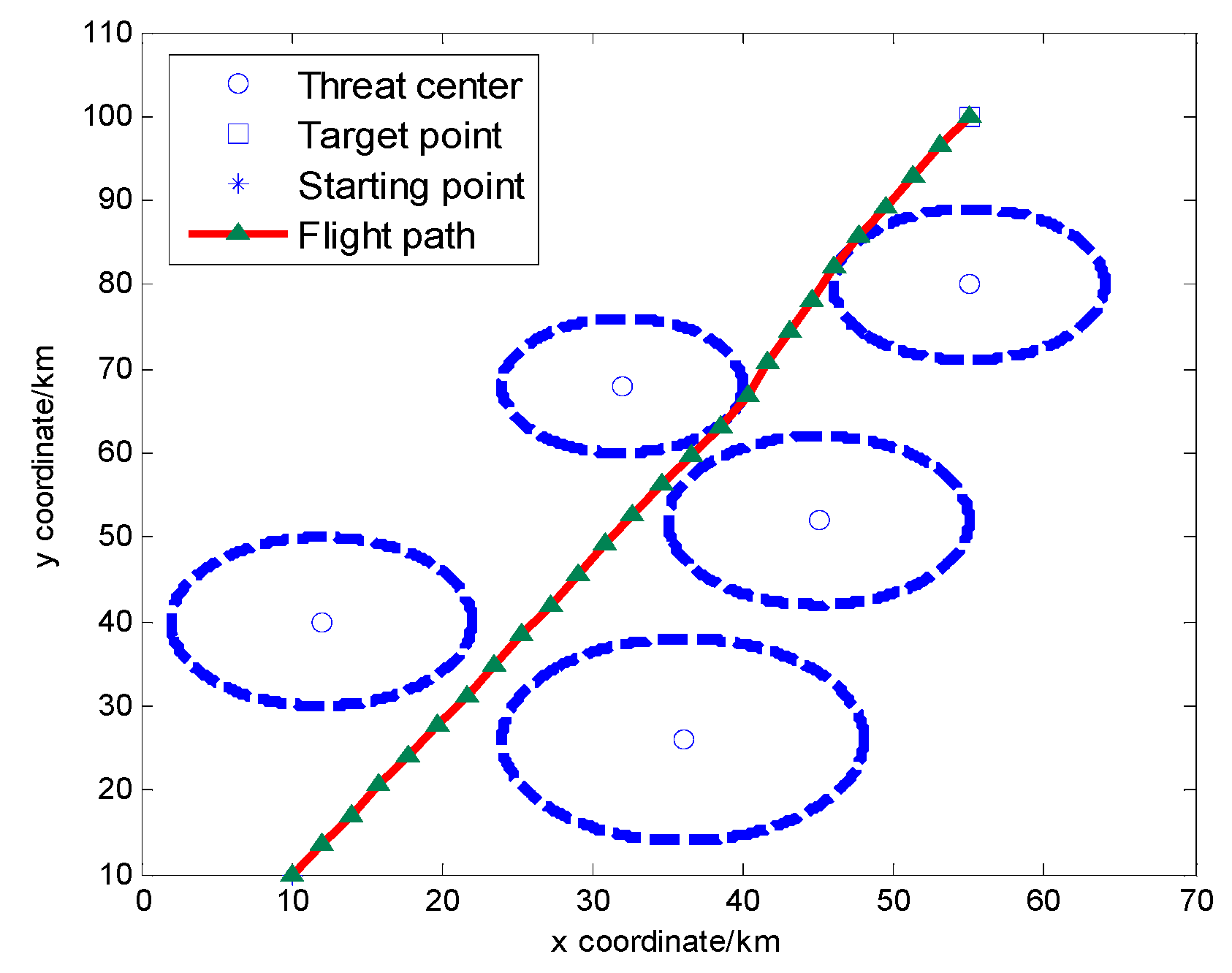
Modeling of threat resources is key for solving the UCAV path-planning problem. In this model, S is defined as the starting point, and T is the target point (Figure 1) [18,19]. There are some threat resources in UCAV battlefield, for example, radars, missiles, and artillery, the effects of which all are shown in the form of a circle. The extent to which UCAV is threatened is proportional to the fourth power of the distance from the threat center. The flight task is to generate an optimal or suboptimal path, so that the UCAV can avoid the threat area from starting point S to the destination T.

Figure 1. Typical Unmanned combat air vehicle (UCAV) Battle Field Model.

Figure 1. Typical Unmanned combat air vehicle (UCAV) Battle Field Model.

There are three main steps in the path planning. First, connect the starting point S and the target point T into a line segment ST. Second, divide the line segment ST into D + 1 equal parts. At each segment point, draw the vertical line of ST, denoted as L₁, L₂,…,L_k,…L_D. Third, take a discrete point in each vertical section L_k, these points constitute a collection of discrete points [19,20] $C=\{S,L_1(x(1),y(1)),L_2(x(2),y(2)),\dots ,L_k(x(k),y(k)),\dots L_D(x(D),y(D)),T\}$. Fourth, connect these discrete points in order to form a path. In this way, the path-planning problem is transformed into the optimal orthogonal coordinate system to achieve the optimization of the objective function.

In order to speed up the search speed of the algorithm, we can take line segment ST as the x-axis and carry on the coordinate transformation on each discrete point (x(k),y(k)) according to Equation (1), where θ is the angle between the original x-axis and the line segment ST, while (x_s,y_s) represents the coordinates of the original coordinate system.

$$\left[\begin{array}{l}x\prime (k)\\ y\prime (k)\end{array}\right]=\left[\begin{array}{l}\cos \mathsf{\theta }\sin \mathsf{\theta }\\ -\sin \mathsf{\theta }\cos \mathsf{\theta }\end{array}\right]\left[\begin{array}{l}x(k)-x_s\\ y(k)-y_s\end{array}\right]$$

(1)

Thus, the x coordinates of each discrete point can be calculated by a simple formula $x\prime (k)=\frac{\left|ST\right|}{D+1}\cdot k$. The set of discrete points C can be simplified to C′ = {0,L₁(y)′(1)),L₂(y′(2)),…,L_k(y′(k)),…L_D(y′(D)),0}, which can greatly reduce the cost of computation.

2.2. Evaluation Function

Evaluation of path planning for UCAV mainly consists of the threat cost J_t and the fuel cost J_f, the formula for calculation is as follows:

$$J_t={\displaystyle \underset{0}{\overset{L}{\int }}{w}_{t}dl}$$

(2)

$$J_f={\displaystyle \underset{0}{\overset{L}{\int }}{w}_{f}dl}$$

(3)

where w_t is the threat cost of each point on the flight path, w_f is the fuel cost for each point on the route, and L is the total length of the route.

In order to improve the computational efficiency, a more accurate approximation strategy can be used. In this work, the threat cost of the route between two discrete points was calculated. It is approximately equal to the sum of the threat cost of five points, as shown in Figure 2 [18,19].

Figure 2. Computation for Threat Cost.

Figure 2. Computation for Threat Cost.

If the i th edge is within the effect range, the calculation formula of the threat cost is as follows:

$$w_{t,L_i}=\frac{L_i}{5}\cdot {\displaystyle \sum _{k=1}^{N_t}{t}_k}\cdot (\frac{1}{d_{0.1,i,k}^4}+\frac{1}{d_{0.3,i,k}^4}+\frac{1}{d_{0.5,i,k}^4}+\frac{1}{d_{0.7,i,k}^4}+\frac{1}{d_{0.9,i,k}^4})$$

(4)

where, N_t is the number of threatening areas, L_i is the i th sub-path length, d_0.1,i,k is the distance from the 1/10 point on the i th edge to the k th threat, and t_k is the threat level of k th threat.

Assuming the speed of a UCAV is a constant, the fuel cost J_f can be equivalent to the total length L of the flight path.

Therefore, the total cost comes from a weighted sum of the threat and fuel cost. It can be defined as Equation (5).

$$J=\text{λ}{J}_t+(1-\text{λ})J_f$$

(5)

where λ is a variable between 0 and 1, which is the balance between safety and fuel performance. If flight security is highly important to this task, we will select a larger λ, while if the speed is vital to the flight task, we will choose a smaller λ. In this paper, λ is equal to 0.5.

3. The Basic Wind Driven Optimization

The inspiration of the proposed WDO derives from the atmosphere. In the atmosphere, wind blows from high-pressure areas to low-pressure areas until the air pressure is balanced. The beginning of WDO algorithm is Newton’s second law of motion [21,22].

$$\mathsf{\rho }\overrightarrow{\omega }={\displaystyle \sum {\overrightarrow{F}}_i}$$

(6)

where, $\overrightarrow{\omega }$ is the acceleration, ρ is the air density for an infinitesimal air parcel, and ${\overrightarrow{F}}_i$ are all the forces acting on the air parcel.

The cause of the air movement is due to the combination of many forces, mainly including gravitational force (${\overrightarrow{F}}_G$), pressure gradient force (${\overrightarrow{F}}_{PG}$), Coriolis force (${\overrightarrow{F}}_C$) and friction force (${\overrightarrow{F}}_F$). The physical equations of the abovementioned forces are as follows:

$${\overrightarrow{F}}_G=\mathsf{\rho \delta }V\overrightarrow{g}$$

(7)

$${\overrightarrow{F}}_{PG}=-\nabla P\mathsf{\delta }V$$

(8)

$${\overrightarrow{F}}_C=-2\text{Ω}\times \overrightarrow{u}$$

(9)

$${\overrightarrow{F}}_F=-\mathsf{\rho \alpha }\overrightarrow{u}$$

(10)

where δV is finite volume of the air, $\overrightarrow{g}$ represents the gravitational acceleration, $\nabla P$ represents the pressure gradient, Ω is rotation of the earth, $\overrightarrow{u}$ represents the velocity vector of the wind and α is the friction coefficient.

The forces mentioned above can be added to the Equation (6). The equation can be described as Equation (11):

$$\mathsf{\rho }\frac{\Delta \overrightarrow{u}}{\Delta t}=\left(\text{ρδ}V\overrightarrow{g}\right)+\left(-\nabla P\text{δ}V\right)+\left(-2\text{Ω}\times \overrightarrow{u}\right)+\left(-\text{ρα}\overrightarrow{u}\right)$$

(11)

where the acceleration $\overrightarrow{\alpha }$ in Equation (11) is rewritten as $\overrightarrow{\alpha }=\Delta \overrightarrow{u}/\Delta t$. For simplicity, set Δt = 1, for an infinitesimal air parcel and set δV = 1, which simplifies Equation (11) to

$$\mathsf{\rho }\Delta \overrightarrow{u}=\left(\mathsf{\rho }\overrightarrow{g}\right)+\left(-\nabla P\right)+\left(-2\text{Ω}\times \overrightarrow{u}\right)+\left(-\text{ρα}\overrightarrow{u}\right)$$

(12)

On the basis of the ideal gas law, Equation (13), the density ρ can be written in terms of the pressure, thus Equation (12) can be rewritten as

$$P=\mathsf{\rho }RT$$

(13)

$$\Delta \overrightarrow{u}=\overrightarrow{g}+\left(-\nabla P\frac{RT}{P_{cur}}\right)+\left(\frac{-2\text{Ω}\times \overrightarrow{u}RT}{P_{cur}}\right)+\left(-\mathsf{\alpha }\overrightarrow{u}\right)$$

(14)

where, P is the pressure, R is the universal gas constant, T is the temperature, and P_cur is the pressure of current location. It is assumed in the WDO algorithm that velocity and position of the air parcel are changing at each iteration. Thus, $\Delta \overrightarrow{u}$ can be written as $\Delta \overrightarrow{u}={\overrightarrow{u}}_{new}-{\overrightarrow{u}}_{cur}$, where ${\overrightarrow{u}}_{new}$ represents the velocity in next iteration and ${\overrightarrow{u}}_{cur}$ is the velocity at the current iteration. $\overrightarrow{g}$ and $\nabla P$ are vectors, they can be broken down in direction and magnitude as $\overrightarrow{g}=\left|g\right|\left(0-x_{cur}\right)$, $-\nabla P=\left|P_{opt}-P_{cur}\right|\left(x_{opt}-x_{cur}\right)$, P_opt is the optimum pressure point that has been found so far, x_opt is the optimum location that has been found so far, and x_cur is the current location, thus updating Equation (14) with the new equations, so that Equation (14) can be rewritten as:

$${\overrightarrow{u}}_{new}=\left(1-\alpha \right){\overrightarrow{u}}_{cur}-g{x}_{cur}+\left(\frac{RT}{P_{cur}}\left|P_{opt}-P_{cur}\right|\left(x_{opt}-x_{cur}\right)\right)+\left(\frac{-2\text{Ω}\times \overrightarrow{u}RT}{P_{cur}}\right)$$

(15)

Finally, there are three additional substitutions needed. First, the influence of the Coriolis force $\left(\text{Ω}\times \overrightarrow{u}\right)$ is replaced by the velocity influence from another dimension ${\overrightarrow{u}}_{cur}^{other\dim }$; second, all the coefficients are combined together, i.e., c = −2RT; and third, in some cases where the pressure is extremely large, the updated velocities are too large to become meaningless, the efficiency of the WDO algorithm will be reduced. Thus, the actual pressure value is replaced by rank among all air parcels based on their pressure values, the resulting equation of updating the velocity can be described as in Equation (16), and the equation of updating the location can be described as in Equation (17).

$${\overrightarrow{u}}_{new}=\left(1-\alpha \right){\overrightarrow{u}}_{cur}-g{x}_{cur}+\left(RT\left|1-\frac{1}{i}\right|\left(x_{opt}-x_{cur}\right)\right)+\left(\frac{c{\overrightarrow{u}}_{cur}^{other\dim }}{i}\right)$$

(16)

$${\overrightarrow{x}}_{new}={\overrightarrow{x}}_{cur}+\left({\overrightarrow{u}}_{new}\times \Delta t\right)$$

(17)

where i is the ranking among all air parcels, ${\overrightarrow{x}}_{new}$ represents the new location for the next iteration.

WDO is similar to other nature-inspired optimization algorithms, but compared to other optimization algorithms, the code of WDO is more simple and easy to implement, as it has less control variables that need to be adjusted.

4. Quantum Computing

In quantum computing, the smallest information unit is a quantum bit, also called a qubit. It uses “0” and “1” to represent the two basic states. The difference between qubit and classical bit is that the qubit not only can be in a state of “0” or “1”, qubit can also be in a state between “0” and “1”. That is, “0” and “1” states exist in a certain probability. The state of a qubit can be described as [23].

$$|\text{Ψ}⟩=\mathsf{\alpha }|0⟩+\mathsf{\beta }|1⟩$$

(18)

where, α and β are a pair of complex numbers. They are called the probability amplitude of qubit. α² and β² represent the probability that the quantum bits are in “0” and “1”, respectively, and satisfy the equation ${\left|\mathsf{\alpha }\right|}^2+{\left|\mathsf{\beta }\right|}^2=1$. $|x⟩$ represents a quantum state.

An n-qubits representation can be defined as

$$\left[\begin{array}{l}{\mathsf{\alpha }}_1\\ {\mathsf{\beta }}_1\end{array}|\begin{array}{l}{\mathsf{\alpha }}_2\\ {\mathsf{\beta }}_2\end{array}|\begin{array}{l}\dots \\ \cdots \end{array}|\begin{array}{l}{\mathsf{\alpha }}_k\\ {\mathsf{\beta }}_k\end{array}|\begin{array}{l}\dots \\ \cdots \end{array}|\begin{array}{l}{\mathsf{\alpha }}_n\\ {\mathsf{\beta }}_n\end{array}|\right]$$

(19)

5. Quantum Wind Driven Optimization

This paper proposed a new quantum-inspired meta-heuristic algorithm, namely quantum wind driven optimization (QWDO). The QWDO uses probability amplitude of qubit to represent the particle’s position. The movement of position can be realized by the quantum rotation gate strategy. Position realizes the mutation using quantum non-gate strategy. This operation can improve the population diversity and avoid premature convergence. Because each qubit has two probability amplitudes, each particle can also represent the two positions of the optimization space. In the case of the same number of particles, the search process can be accelerated.

5.1. Generate Initial Population

Because the probability amplitude satisfies the equation ${\left|\mathsf{\alpha }\right|}^2+{\left|\mathsf{\beta }\right|}^2=1$, we let $\mathsf{\alpha }=\cos (\mathsf{\theta })$, and $\mathsf{\beta }=\sin (\mathsf{\theta })$ [17]. Where, □ is a rotation angle. The coding scheme is as following:

$$P=\left[\begin{array}{l}cos({\mathsf{\theta }}_{i1})\\ sin({\mathsf{\theta }}_{i1})\end{array}|\begin{array}{l}cos({\mathsf{\theta }}_{i2})\\ sin({\mathsf{\theta }}_{i2})\end{array}|\begin{array}{l}\dots \\ \cdots \end{array}|\begin{array}{l}cos({\mathsf{\theta }}_{ik})\\ sin({\mathsf{\theta }}_{ik})\end{array}|\begin{array}{l}\dots \\ \cdots \end{array}|\begin{array}{l}cos({\mathsf{\theta }}_{in})\\ sin({\mathsf{\theta }}_{in})\end{array}|\right]$$

(20)

where, □_ij = 2π × rand, rand is a random number between 0 and 1, i = 1,2,…,m; j = 1,2,…,n; m is the size of the population, and n is the space dimension. Each individual corresponds to the two position of the problem space. That is, the probability amplitude of quantum state $|0⟩$ and $|1⟩$:

$$P_{ic}=(cos({\mathsf{\theta }}_{i1}),cos({\mathsf{\theta }}_{i2}),\dots ,cos({\mathsf{\theta }}_{in}))$$

(21)

$$P_{is}=(\sin ({\mathsf{\theta }}_{i1}),\sin ({\mathsf{\theta }}_{i2}),\dots ,\sin ({\mathsf{\theta }}_{in}))$$

(22)

where P_ic is a cosine position and P_is is a sinusoidal position.

5.2. Transformation of the Solution Space

In order to calculate the current position of the particle, there is a need to carry out the transformation of the space. We need to map the two positions of the particles from the unit space $I={\left[-1,1\right]}^n$ to the solution space of the optimization problem. The variables of solution space are as follows:

$$X_{ic}^j=\frac{1}{2}[X_{\max }(1+{\mathsf{\alpha }}_i^j)+X_{\min }(1-{\mathsf{\alpha }}_i^j)]$$

(23)

$$X_{is}^j=\frac{1}{2}[X_{\max }(1+{\mathsf{\beta }}_i^j)+X_{\min }(1-{\mathsf{\beta }}_i^j)]$$

(24)

where, $X_{ic}^j$ is calculated by the probability amplitude ${\alpha }_i^j$ of quantum state $|0⟩$ and $X_{is}^j$ is calculated by the probability amplitude ${\mathsf{\beta }}_i^j$ of quantum state $|1⟩$.

5.3. Updating Process

In order to prevent the algorithm from falling into local optimum, in this paper, two quantum gate strategies are applied. The movement of position can be realized by the quantum rotation gate strategy, and position realizes the mutation using quantum non-gate strategy.

5.3.1. Updating Formulas of Phase Angle Increment and Phase Angle

In quantum wind driven optimization (QWDO), updating formulas of phase angle increment and phase angle are as following:

$$\begin{array}{l}\Delta {\mathsf{\theta }}_{ij}(t+1)=\left(1-\mathsf{\alpha }\right)\ast \Delta {\mathsf{\theta }}_{ij}(t)-g\ast \cos \left(\Delta {\mathsf{\theta }}_{ij}(t)\right)+\\ \left[\left|1-\frac{1}{r}\right|RT\ast \left(\cos \left(\Delta {\mathsf{\theta }}_{opt}(t)\right)-\cos \left(\Delta {\mathsf{\theta }}_{ij}(t)\right)\right)\right]+\frac{c\ast \Delta {\mathsf{\theta }}_{rand}(t)}{r}\end{array}$$

(25)

$${\mathsf{\theta }}_{ij}(t+1)={\mathsf{\theta }}_{ij}(t)+\Delta {\mathsf{\theta }}_{ij}(t+1)$$

(26)

where, Δθ_ij and θ_ij are the j th dimension of the i th phase angle increment and phase angle, respectively.

5.3.2. Quantum Rotation Gate Strategy

This paper uses quantum rotation gate strategy to update the probability amplitude.

$$\left[\begin{array}{l}\cos ({\mathsf{\theta }}_{ij}(t+1))\\ \sin ({\mathsf{\theta }}_{ij}(t+1))\end{array}\right]=\left[\begin{array}{l}\cos (\Delta {\mathsf{\theta }}_{ij}(t+1))-\sin (\Delta {\mathsf{\theta }}_{ij}(t+1))\\ \sin (\Delta {\mathsf{\theta }}_{ij}(t+1))\cos (\Delta {\mathsf{\theta }}_{ij}(t+1))\end{array}\right]\left[\begin{array}{l}\cos ({\mathsf{\theta }}_{ij}(t))\\ \sin ({\mathsf{\theta }}_{ij}(t))\end{array}\right]=\left[\begin{array}{l}\cos ({\mathsf{\theta }}_{ij}(t)+\Delta {\mathsf{\theta }}_{ij}(t+1))\\ \sin ({\mathsf{\theta }}_{ij}(t))+\Delta {\mathsf{\theta }}_{ij}(t+1)\end{array}\right]$$

(27)

Two updated positions are as follows:

$$\widetilde{P_{ic}}=(\cos ({\mathsf{\theta }}_{ij}(t)+\Delta {\mathsf{\theta }}_{ij}(t+1)),\dots ,\cos ({\mathsf{\theta }}_{ij}(t)+\Delta {\mathsf{\theta }}_{ij}(t+1)))$$

(28)

$$\widetilde{P_{is}}=(\sin ({\mathsf{\theta }}_{ij}(t))+\Delta {\mathsf{\theta }}_{ij}(t+1),\dots ,\sin ({\mathsf{\theta }}_{ij}(t))+\Delta {\mathsf{\theta }}_{ij}(t+1))$$

(29)

5.3.3. Quantum Non-Gate Strategy

This paper uses quantum non-gate strategy to make the position mutation. This operation can increase the population diversity and avoid premature convergence. rand_i is a random number between 0 and 1. If rand_i < P_m, where P_m is the mutation rate, it will exchange two probability amplitudes. The exchange formula is as follows:

$$\left[\begin{array}{l}01\\ 10\end{array}\right]\left[\begin{array}{l}\cos ({\mathsf{\theta }}_{ij})\\ \sin ({\mathsf{\theta }}_{ij})\end{array}\right]=\left[\begin{array}{l}\sin ({\mathsf{\theta }}_{ij})\\ \cos ({\mathsf{\theta }}_{ij})\end{array}\right]=\left[\begin{array}{l}\cos ({\mathsf{\theta }}_{ij}+\frac{\pi }{2})\\ \sin ({\mathsf{\theta }}_{ij}+\frac{\pi }{2})\end{array}\right]$$

(30)

5.4. The Flow Chart of QWDO

Algorithm 1. Quantum Wind Driven Optimization (QWDO) Algorithm.

Step 1. Initialize parameters. N (Population size); G (Max number of generations); RT (RT coefficient); α (The friction coefficient); g (Gravitational constant); c (Constant in the update equation); max V (Maximum allowed speed); Pm (Mutation scale factor). Step 2. Generate Initial Population. Step 3. Transform the solution space according to Equations (23) and (24). Step 4. Evaluate fitness of each air parcel. Step 5. Identify the best solution among all air parcels. Step 6. While stopping criterion is not satisfied Step 6.1. Update phase angle increment and phase angle by Equations (25) and (26) Step 6.2. Update the probability amplitude by using quantum rotation gate strategy according to Equation (27). Step 6.3. If rand Pm then Implement quantum non-gate strategy by Equation (30). End if Step 6.4. Transform the solution space according to Equations (23) and (24). Step 6.5. Evaluate fitness of each air parcel. Step 6.6.Identify the best solution among all air parcels. Step 6.7.Increment the generation count G = G + 1. Step 7. End while

5.5. The Flow Chart of QWDO for UCAV Path Planning

Algorithm 2. QWDO for UCAV Path Planning Algorithm.

Step 1. Initialize parameters. N (Population size); G (Max number of generations); RT (RT coefficient); α (The friction coefficient); g (Gravitational constant); c (Constant in the update equation); Pm (Mutation scale factor). Step 2. Build the UCAV battlefield model. Step 3. Transform coordinate system according to Equation (1). Step 4. Generate Initial Population according to Equation (20). Step 5. Transform the solution space according to Equations (23) and (24). Step 6. Evaluate the cost of each flight path by Equation (5). Step 7. Get the best path. Step 8. While stopping criterion is not satisfied Step 8.1. Update phase angle increment and phase angle by Equation (25) and (26). Step 8.2. Update the probability amplitude by using quantum rotation gate strategy according to Equation (27). Step 8.3. If rand < Pm then Implement quantum non-gate strategy by Equation (30). End if Step 8.4. Transform the solution space according to Equations (23) and (24). Step 8.5. Evaluate the cost of each flight path by Equation (5). Step 8.6. Get the best path. Step 8.7. Increment the generation count G = G + 1. Step 9. End while

6. Experimental Results

6.1. Experimental Setup

All algorithms are implemented in MATLAB R2012a (MathWorks, New York, USA, 2012), and experiments are performed on a Pentium 3.00 GHz Processor (Intel, New York, NY, USA, 2004), with 4.0 GB of memory, Windows 7 operating system.

6.2. Parameters Setting

In this section, the parameters setting are presented. Table 1, Table 2, Table 3, Table 4, Table 5, Table 6 and Table 7 represent the necessary parameters used for QWDO, QBA, QPSO, WDO, BA, PSO and DE algorithms, respectively. Bayraktar et al. did a lot of research for the parameters setting of WDO algorithm [10]. The parameters for the set of quantum algorithms are the same as the original algorithm. The parameters set for some algorithms are based on the practical experience to take the appropriate value. In all trials, the population size is 30 (Popsize = 30).

Table 1. The parameters setting of quantum wind driven optimization (QWDO).

Parameters	Value
RT coefficient	1
Constants in the update equation	0.8
Maximum allowed speed	0.3
Gravitational constant	0.6
Coriolis effect	0.7
The range of phase angle	[−π,π]

Table 1. The parameters setting of quantum wind driven optimization (QWDO).

Parameters	Value
RT coefficient	1
Constants in the update equation	0.8
Maximum allowed speed	0.3
Gravitational constant	0.6
Coriolis effect	0.7
The range of phase angle	[−π,π]

Table 2. The parameters setting of quantum bat algorithm (QBA).

Parameters	Value
Pulse frequency range	[0,2]
Maximum pulse emission	0.5
The maximum loudness	0.5
Attenuation coefficient of loudness	0.95
Increasing coefficient of pulse emission	0.05
The range of phase angle	[−π,π]

Table 2. The parameters setting of quantum bat algorithm (QBA).

Parameters	Value
Pulse frequency range	[0,2]
Maximum pulse emission	0.5
The maximum loudness	0.5
Attenuation coefficient of loudness	0.95
Increasing coefficient of pulse emission	0.05
The range of phase angle	[−π,π]

Table 3. The parameters setting of quantum particle swarm optimization (QPSO).

Parameters	Value
Constant inertia	0.7298
The first acceleration coefficients	1.4962
The second Acceleration coefficients	1.4962
The range of phase angle	[−π,π]

Table 3. The parameters setting of quantum particle swarm optimization (QPSO).

Parameters	Value
Constant inertia	0.7298
The first acceleration coefficients	1.4962
The second Acceleration coefficients	1.4962
The range of phase angle	[−π,π]

Table 4. The parameters setting of wind driven optimization (WDO).

Parameters	Value
RT coefficient	1
Constants in the update equation	0.8
Maximum allowed speed	0.3
Gravitational constant	0.6
Coriolis effect	0.7

Table 4. The parameters setting of wind driven optimization (WDO).

Parameters	Value
RT coefficient	1
Constants in the update equation	0.8
Maximum allowed speed	0.3
Gravitational constant	0.6
Coriolis effect	0.7

Table 5. The parameters setting of bat algorithm (BA).

Parameters	Value
Pulse frequency range	[0,2]
Maximum pulse emission	0.5
The maximum loudness	0.5
Attenuation coefficient of loudness	0.95
Increasing coefficient of pulse emission	0.05

Table 5. The parameters setting of bat algorithm (BA).

Parameters	Value
Pulse frequency range	[0,2]
Maximum pulse emission	0.5
The maximum loudness	0.5
Attenuation coefficient of loudness	0.95
Increasing coefficient of pulse emission	0.05

Table 6. The parameters setting of particle swarm optimization (PSO).

Parameters	Value
Constant inertia	0.7298
The first acceleration coefficients	1.4962
The second Acceleration coefficients	1.4962

Table 6. The parameters setting of particle swarm optimization (PSO).

Parameters	Value
Constant inertia	0.7298
The first acceleration coefficients	1.4962
The second Acceleration coefficients	1.4962

Table 7. The parameters setting of difference evolution (DE).

Parameters	Value
Mutation scale factor	0.2
Crossover probability	0.03

Table 7. The parameters setting of difference evolution (DE).

Parameters	Value
Mutation scale factor	0.2
Crossover probability	0.03

6.3. Experimental Results

This section is mainly to test the performance of the QWDO algorithm for solving the problem of UCAV path planning. In this section, a total of two test instances were carried out. In the simulation experiment, the dimension D and the maximum number of iterations Maxgen are used as the two control variables. We look at the performance of QWDO algorithm as compared with other optimization algorithms, for instance, quantum bat algorithm (QBA) [24], quantum particle swarm optimization (QPSO) [25], wind driven optimization (WDO), bat algorithm (BA), particle swarm optimization (PSO), and differential evolution (DE). All of the test cases are carried out with 50 independent experiments.

We use the battlefield environment parameters described in [5]. UCAV starts at (10,10) and the destination is (55,100). In this battlefield environment, there are five threat centers. Table 8 presents information about known threats for the first test instance.

Table 8. Information about known threats for the first test instance.

Threat Center (km)	(45,50)	(12,40)	(32,68)	(36,26)	(55,80)
Threat radius (km)	10	10	8	12	9
Threat grade	2	10	1	2	3

Table 8. Information about known threats for the first test instance.

Threat Center (km)	(45,50)	(12,40)	(32,68)	(36,26)	(55,80)
Threat radius (km)	10	10	8	12	9
Threat grade	2	10	1	2	3

Unmanned combat air vehicle (UCAV) path planning aims to calculate the optimal or suboptimal flight path. When the dimension of the algorithm is not the same, the results will be different. Table 9 shows the mean results, the best fitness value and the worst fitness value between the algorithms of 50 independent runs. In the following tables, bold results indicate that the algorithm performed the best.

From Table 9, we see that the mean normalized optimization results of DE algorithm performed the best in D = 5 and D = 10. In the rest of the cases, the mean normalized optimization results of QWDO algorithm performed best. We can see that the best-normalized optimization results of DE algorithm performed the best in D = 5, and in the rest of the cases, the best normalized optimization results of QWDO algorithm performed best. As can be seen in Table 9, the worst normalized optimization results of QWDO algorithm is the best, except in D = 15 and D = 25. In summary, the performance of QWDO algorithm is better than other optimization algorithms.

Table 9. Experimental results for the first test instance in different D.

Popsize	Maxgen	D	Result	DE	PSO	BA	WDO	QPSO	QBA	QWDO
30	200	5	Mean	59.47631887	69.69789792	79.69109684	71.34530853	63.43087561	68.98614459	68.96129066
			Best	53.50706462	53.78972474	53.65716479	69.87539134	53.51528812	53.71340066	57.98320586
			Worst	69.41083451	122.5251479	153.561503	74.74310818	69.65781726	69.70146844	69.34914343
30	200	10	Mean	51.65071551	51.46197291	51.63995084	52.22163684	51.09958359	51.09603877	50.7143172
			Best	50.71342237	50.76572646	50.75929951	51.70051826	50.73093318	50.74767855	50.7133255
			Worst	56.58333938	54.59093708	63.46628192	52.82754363	53.39086949	53.84706658	50.7210475
30	200	15	Mean	50.66037482	51.5051898	51.87380989	52.44224824	50.76853918	50.89080424	50.58231653
			Best	50.44414089	50.71382405	50.50789696	51.60523312	50.48866711	50.49293993	50.44266169
			Worst	53.13768683	55.0444921	60.46255447	53.11065178	53.31076469	53.69423022	54.54535767
30	200	20	Mean	50.72261529	51.45672198	53.35967758	52.97445056	51.07754398	51.0110708	50.99002665
			Best	50.44379211	50.80930764	50.63331206	52.06541936	50.48490215	50.54761522	50.39488366
			Worst	53.01708277	53.35679952	62.1522776	54.06882944	53.41618848	53.19280513	52.87373122
30	200	25	Mean	51.28794992	51.7891286	53.92302186	53.73746145	52.16273619	52.02298198	50.91502774
			Best	50.48966734	50.99255379	50.80805259	51.49756894	50.92275235	50.67574917	50.38774681
			Worst	57.87611595	54.01746732	58.78868887	54.84758084	54.91448413	54.12956224	55.70310267

DE: difference evolution; PSO: particle swarm optimization; BA: bat algorithm; WDO: wind driven optimization; QPSO: quantum particle swarm optimization; QBA: quantum bat algorithm; QWDO: quantum wind driven optimization.

Table 9. Experimental results for the first test instance in different D.

Popsize	Maxgen	D	Result	DE	PSO	BA	WDO	QPSO	QBA	QWDO
30	200	5	Mean	59.47631887	69.69789792	79.69109684	71.34530853	63.43087561	68.98614459	68.96129066
			Best	53.50706462	53.78972474	53.65716479	69.87539134	53.51528812	53.71340066	57.98320586
			Worst	69.41083451	122.5251479	153.561503	74.74310818	69.65781726	69.70146844	69.34914343
30	200	10	Mean	51.65071551	51.46197291	51.63995084	52.22163684	51.09958359	51.09603877	50.7143172
			Best	50.71342237	50.76572646	50.75929951	51.70051826	50.73093318	50.74767855	50.7133255
			Worst	56.58333938	54.59093708	63.46628192	52.82754363	53.39086949	53.84706658	50.7210475
30	200	15	Mean	50.66037482	51.5051898	51.87380989	52.44224824	50.76853918	50.89080424	50.58231653
			Best	50.44414089	50.71382405	50.50789696	51.60523312	50.48866711	50.49293993	50.44266169
			Worst	53.13768683	55.0444921	60.46255447	53.11065178	53.31076469	53.69423022	54.54535767
30	200	20	Mean	50.72261529	51.45672198	53.35967758	52.97445056	51.07754398	51.0110708	50.99002665
			Best	50.44379211	50.80930764	50.63331206	52.06541936	50.48490215	50.54761522	50.39488366
			Worst	53.01708277	53.35679952	62.1522776	54.06882944	53.41618848	53.19280513	52.87373122
30	200	25	Mean	51.28794992	51.7891286	53.92302186	53.73746145	52.16273619	52.02298198	50.91502774
			Best	50.48966734	50.99255379	50.80805259	51.49756894	50.92275235	50.67574917	50.38774681
			Worst	57.87611595	54.01746732	58.78868887	54.84758084	54.91448413	54.12956224	55.70310267

DE: difference evolution; PSO: particle swarm optimization; BA: bat algorithm; WDO: wind driven optimization; QPSO: quantum particle swarm optimization; QBA: quantum bat algorithm; QWDO: quantum wind driven optimization.

Figure 3, Figure 4, Figure 5, Figure 6 and Figure 7 show the UCAV flight path obtained by the QWDO algorithm testing the first test instance on different D. We can find that the flight path is composed of D equal parts. For all cases in the first instance, the QWDO algorithm can find the flight path that avoids the threat areas with the smallest threat cost.

Figure 3. Result of the first instance for D = 5.

Figure 3. Result of the first instance for D = 5.

Figure 4. Result of the first instance for D = 10.

Figure 4. Result of the first instance for D = 10.

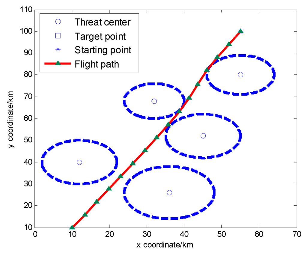
Figure 5. Result of the first instance for D = 15.

Figure 5. Result of the first instance for D = 15.

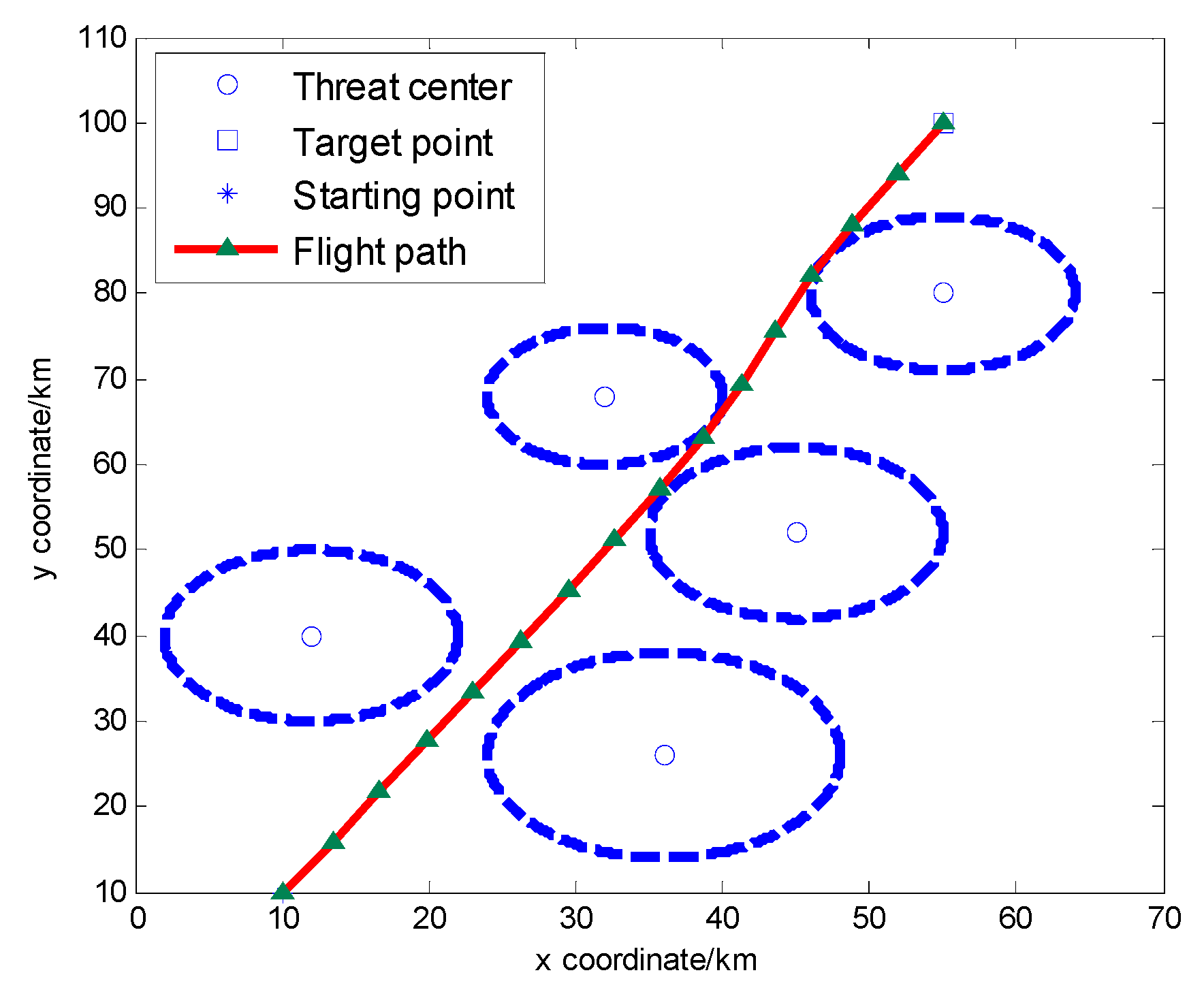
Figure 6. Result of the first instance for D = 20.

Figure 6. Result of the first instance for D = 20.

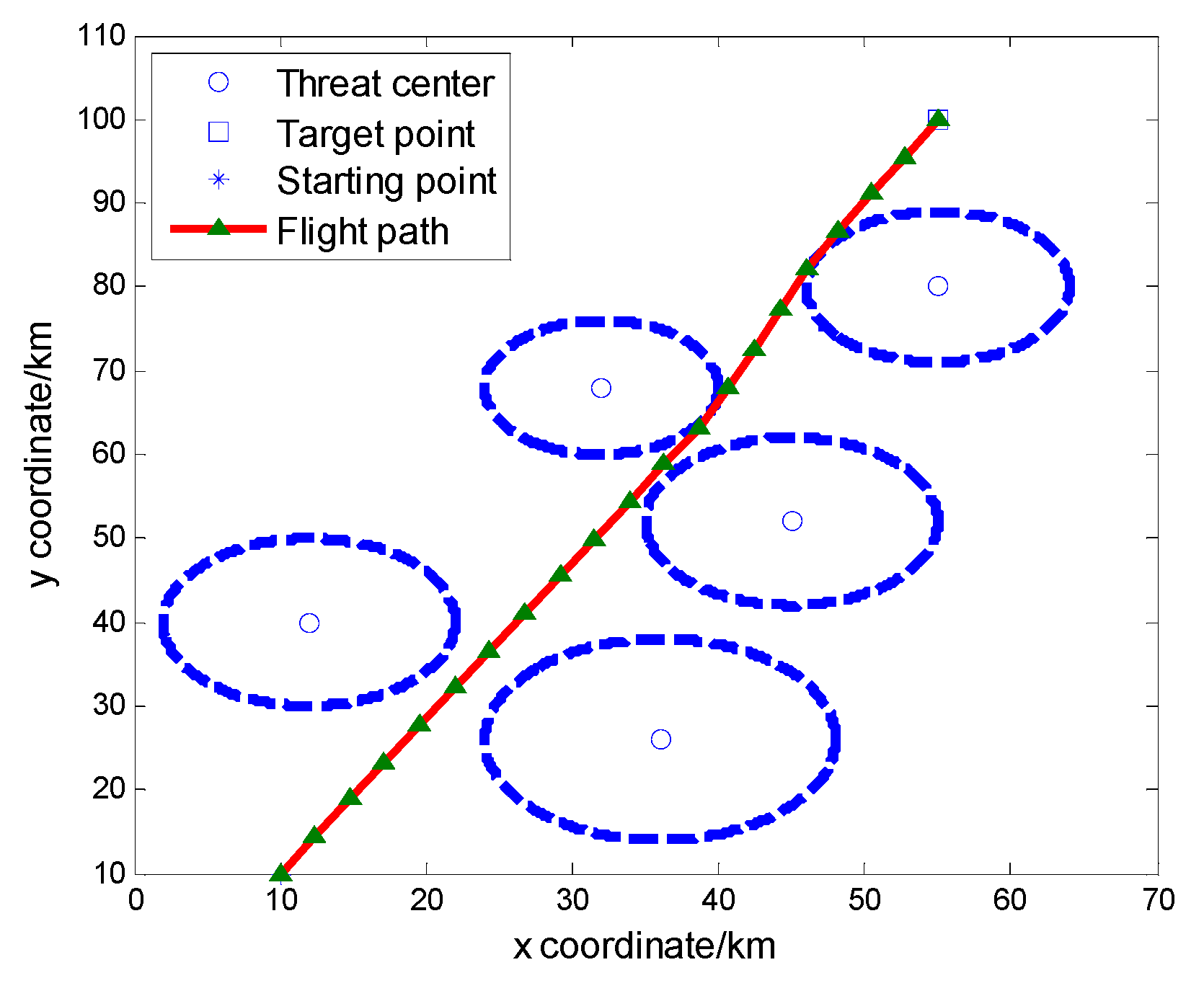
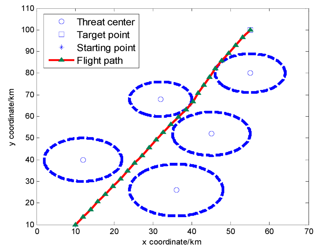
Figure 7. Result of the first instance for D = 25.

Figure 7. Result of the first instance for D = 25.

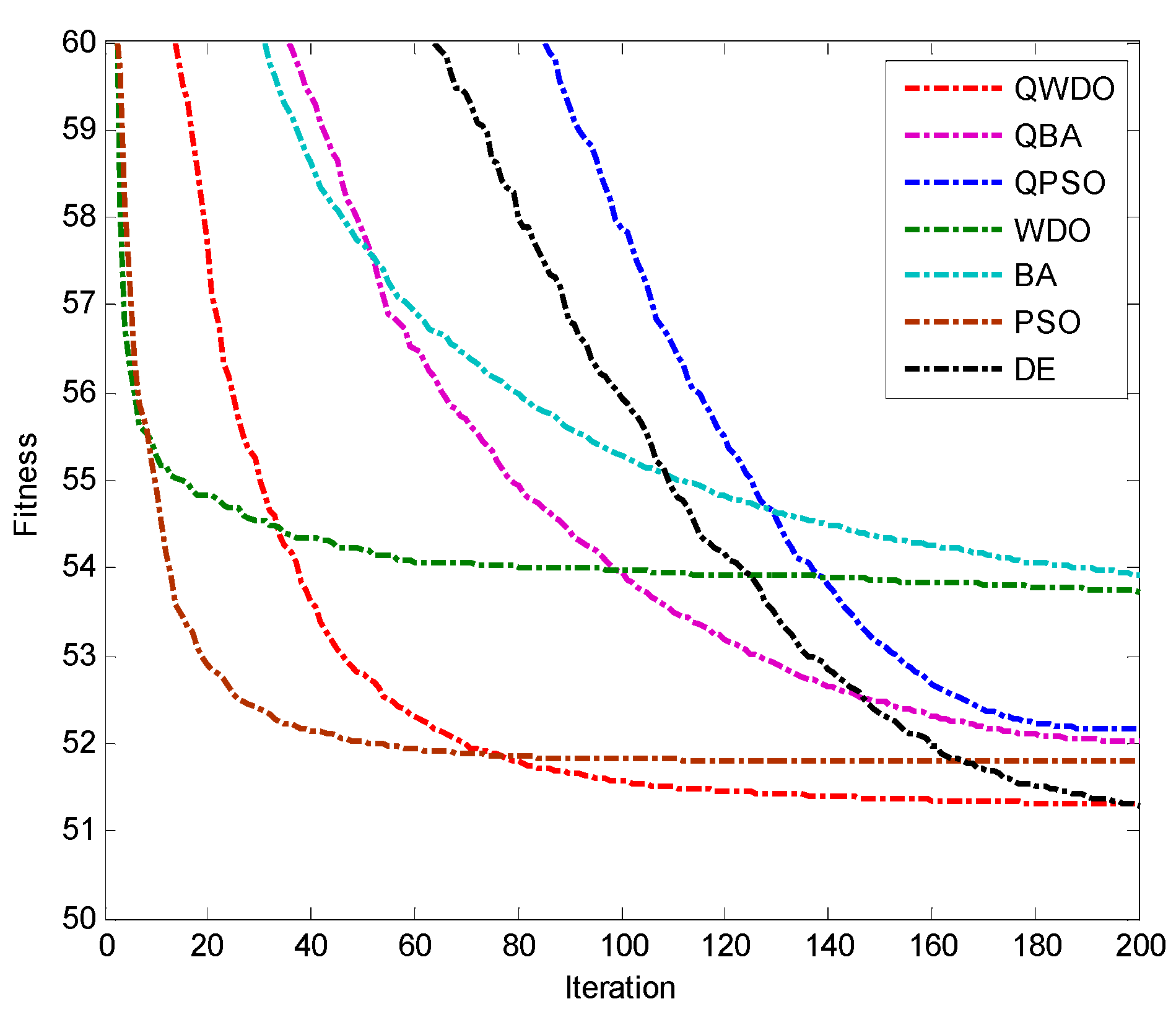
Meanwhile, Figure 8, Figure 9, Figure 10, Figure 11 and Figure 12 have shown evolutionary process of fitness value on different D. In Figure 8, Figure 9, Figure 10, Figure 11 and Figure 12, we can see that QWDO algorithm has a faster global convergence speed and higher convergence precision, except D = 5 and D = 20.

When the maximum number of iterations is not the same, the results will also be different. Table 10 shows the mean results, the best fitness value and the worst fitness value between the algorithms of 50 independent runs. In the following tables, bold results indicate that the algorithm performed the best.

Figure 8. Fitness of the first instance for D = 5.

Figure 8. Fitness of the first instance for D = 5.

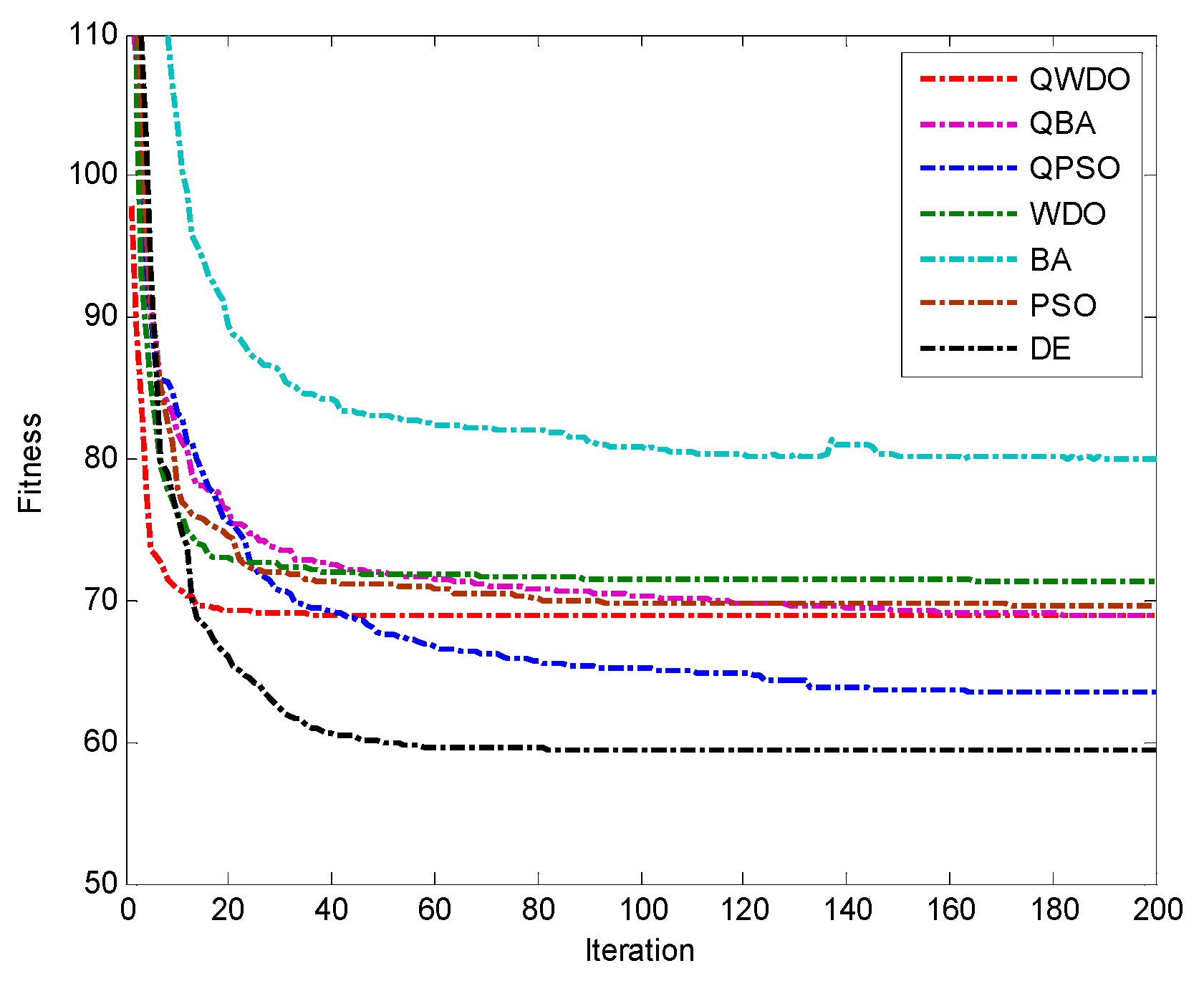
Figure 9. Fitness of the first instance for D = 10.

Figure 9. Fitness of the first instance for D = 10.

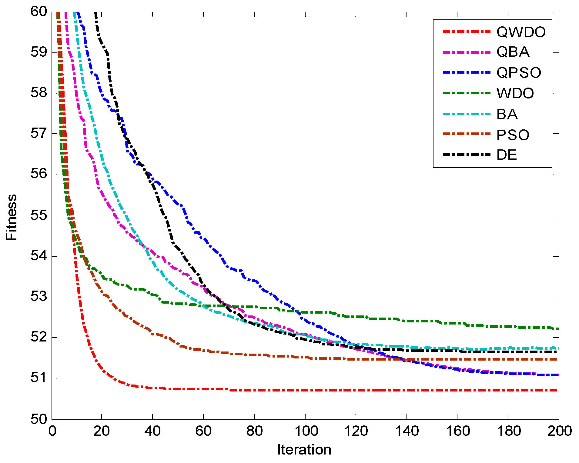
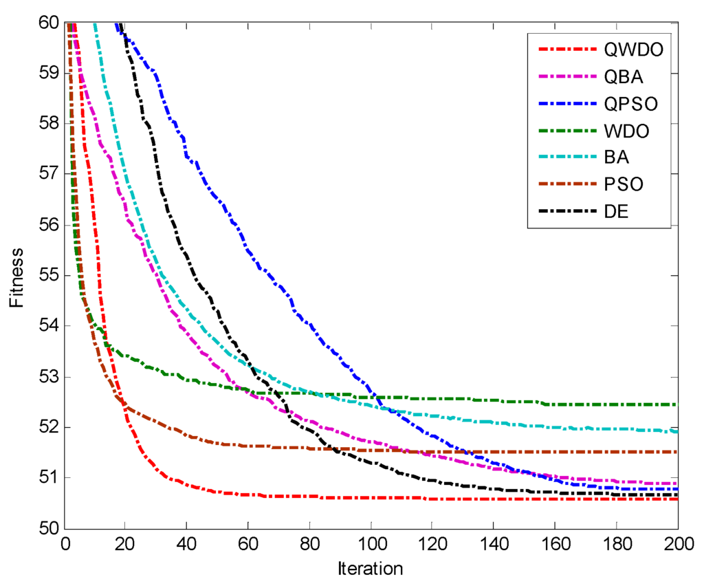
Figure 10. Fitness of the first instance for D = 15.

Figure 10. Fitness of the first instance for D = 15.

In Table 10, we can see that the mean normalized optimization results of QWDO algorithm on UCAV path planning problem performs the best, except in Maxgen = 250. We can see in Table 10, in all different Maxgen, the best-normalized optimization results of QWDO algorithm on UCAV path planning problem are the best. As can be seen in the Table 10, although the worst normalized optimization results of QWDO algorithm in Maxgen = 50 and Maxgen = 100 is not the best, in the rest of the cases, QWDO algorithm performed best. Through the above data we can find QWDO algorithm is very efficient in solving the UCAV path-planning problem. The performance of QWDO is better than other optimization algorithms.

The experimental results of the first test instance show that the QWDO algorithm has fast convergence rate, high convergence precision, and it is an effective and feasible solution in solving the UCAV path-planning problem.

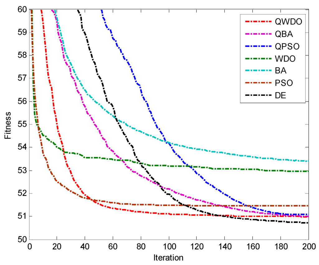
Figure 11. Fitness of the first instance for D = 20.

Figure 11. Fitness of the first instance for D = 20.

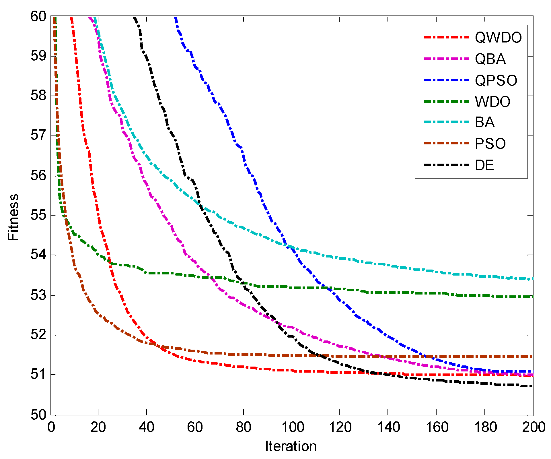
Figure 12. Fitness of the first instance for D = 25.

Figure 12. Fitness of the first instance for D = 25.

In order to verify the performance of the QWDO algorithm for solving the problem of UCAV path planning more fully, in this section, all the algorithms are applied to the second test instance. Similarly, the dimension D and the maximum number of iterations Maxgen are used as the two control variables. We look at the performance of QWDO algorithm as compared with other optimization algorithms, such as, quantum bat algorithm (QBA), quantum particle swarm optimization (QPSO), wind driven optimization (WDO), bat algorithm (BA), particle swarm optimization (PSO), and differential evolution (DE).

In the second test instance, UCAV starts at (10,15) and finishes at (80,75). In this battlefield environment, there are eight threat centers. Table 11 shows information about known threats for the second test instance.

Table 10. Experimental results for the first test instance in different Maxgen.

Popsize	Maxgen	D	Result	DE	PSO	BA	WDO	QPSO	QBA	QWDO
30	50	20	Mean	51.55066072	57.49611763	55.52925757	53.37244656	55.06247744	53.26816353	51.0384824
			Best	50.86230831	52.4021891	50.8335776	51.63208235	52.87505334	51.2628276	50.56417883
			Worst	52.97970342	67.05488964	63.29522516	54.20131962	61.773734	58.6281585	53.31025066
30	100	20	Mean	51.51743739	52.44222368	53.18924498	53.40007277	52.13986363	51.53347574	51.04911419
			Best	50.98301911	50.68878829	51.00545315	51.88063479	51.22499096	50.67123961	50.39932388
			Worst	52.51570068	59.61227827	58.92518468	54.23101102	54.12993175	55.38455421	52.93418088
30	150	20	Mean	51.93773208	50.91881032	53.00666682	53.14375161	51.37913337	51.48087993	50.76428055
			Best	50.76460097	50.41768377	50.6384468	51.90565475	50.63851986	50.61691071	50.39664491
			Worst	59.1205155	53.27343125	61.22625354	54.01364469	55.1714668	54.98546674	52.91230338
30	200	20	Mean	50.73461503	51.67395413	53.26005394	53.15550115	51.39219052	51.02583378	50.58751325
			Best	50.4160651	50.91067104	50.62680554	52.15259159	50.51985597	50.5578439	50.39570371
			Worst	53.33085477	54.17616743	61.10842324	54.17028213	53.93215589	53.50379863	52.86341706
30	250	20	Mean	51.46928513	50.7031705	52.63088516	52.89985245	50.88980761	51.34376512	50.91479454
			Best	50.78648292	50.42161575	50.5392192	51.96380792	50.49328732	50.49715669	50.39447178
			Worst	54.08790265	53.06705989	60.68415725	53.67059243	53.42973728	57.02850459	52.8744808

Table 10. Experimental results for the first test instance in different Maxgen.

Popsize	Maxgen	D	Result	DE	PSO	BA	WDO	QPSO	QBA	QWDO
30	50	20	Mean	51.55066072	57.49611763	55.52925757	53.37244656	55.06247744	53.26816353	51.0384824
			Best	50.86230831	52.4021891	50.8335776	51.63208235	52.87505334	51.2628276	50.56417883
			Worst	52.97970342	67.05488964	63.29522516	54.20131962	61.773734	58.6281585	53.31025066
30	100	20	Mean	51.51743739	52.44222368	53.18924498	53.40007277	52.13986363	51.53347574	51.04911419
			Best	50.98301911	50.68878829	51.00545315	51.88063479	51.22499096	50.67123961	50.39932388
			Worst	52.51570068	59.61227827	58.92518468	54.23101102	54.12993175	55.38455421	52.93418088
30	150	20	Mean	51.93773208	50.91881032	53.00666682	53.14375161	51.37913337	51.48087993	50.76428055
			Best	50.76460097	50.41768377	50.6384468	51.90565475	50.63851986	50.61691071	50.39664491
			Worst	59.1205155	53.27343125	61.22625354	54.01364469	55.1714668	54.98546674	52.91230338
30	200	20	Mean	50.73461503	51.67395413	53.26005394	53.15550115	51.39219052	51.02583378	50.58751325
			Best	50.4160651	50.91067104	50.62680554	52.15259159	50.51985597	50.5578439	50.39570371
			Worst	53.33085477	54.17616743	61.10842324	54.17028213	53.93215589	53.50379863	52.86341706
30	250	20	Mean	51.46928513	50.7031705	52.63088516	52.89985245	50.88980761	51.34376512	50.91479454
			Best	50.78648292	50.42161575	50.5392192	51.96380792	50.49328732	50.49715669	50.39447178
			Worst	54.08790265	53.06705989	60.68415725	53.67059243	53.42973728	57.02850459	52.8744808

Table 11. Information about known threats for the second test instance.

Threat Center	(59,52)	(55,80)	(27,58)	(24,33)	(12,48)	(70,65)	(70,34)	(30,70)
Threat radius	10	9	9	9	12	7	12	10
Threat level	9	7	3	12	1	5	13	2

Table 11. Information about known threats for the second test instance.

Threat Center	(59,52)	(55,80)	(27,58)	(24,33)	(12,48)	(70,65)	(70,34)	(30,70)
Threat radius	10	9	9	9	12	7	12	10
Threat level	9	7	3	12	1	5	13	2

First, the performance of each algorithm is tested in different D. The mean results, the best fitness value and the worst fitness value between the algorithms of 50 independent runs are shown in Table 12. In the following table, bold results indicate that the algorithm performed the best.

According to Table 12, we can see that the mean normalized optimization results of QPSO algorithm on UCAV path planning problem is the best in D = 5 and D = 10. However, in the rest of the cases, QWDO algorithm performed best. We can see that the best-normalized optimization results of QWDO algorithm on UCAV path planning problem are all the best. What is more, the worst normalized optimization results of QWDO algorithm are all the best. As we can see from Table 12, in all cases, the presented global optimization algorithm QWDO algorithm is better than the original WDO algorithm. It shows that the QWDO algorithm is effective in improving the WDO algorithm.

When the maximum number of iterations is different, the results will also be different. Second, the performance of each algorithm is tested in different Maxgen, and the results of the simulation experiment are shown in Table 13. In the following table, bold results indicate that the algorithm performed the best.

From Table 13, we can see that the mean normalized optimization results of QWDO algorithm on the UCAV path-planning problem is always the best. In all different Maxgen cases, the best-normalized optimization results of QWDO algorithm on the UCAV path-planning problem are also the best. As can be seen in Table 13, the worst normalized optimization results of QWDO algorithm also performed best. Through the above data we can find QWDO algorithm is better than other intelligent algorithms in global search and local search. QWDO algorithm is very efficient in solving the UCAV path-planning problem.

Figure 13, Figure 14, Figure 15, Figure 16 and Figure 17 show the UCAV flight path obtained by the QWDO algorithm testing the second test instance on different Maxgen. For all cases in the second test instance, the QWDO algorithm can find the flight path that avoids the threat areas with the smallest threat cost.

Figure 18, Figure 19, Figure 20, Figure 21 and Figure 22 show the evolutionary process of fitness value on different Maxgen. As can be seen in Figure 18, Figure 19, Figure 20, Figure 21 and Figure 22, QWDO algorithm has the fastest convergence speed and the highest convergence precision in all of these tests. It shows the QWDO algorithm has a strong ability to find the optimal solutions.

Figure 13. Result of the second instance for Maxgen = 50.

Figure 13. Result of the second instance for Maxgen = 50.

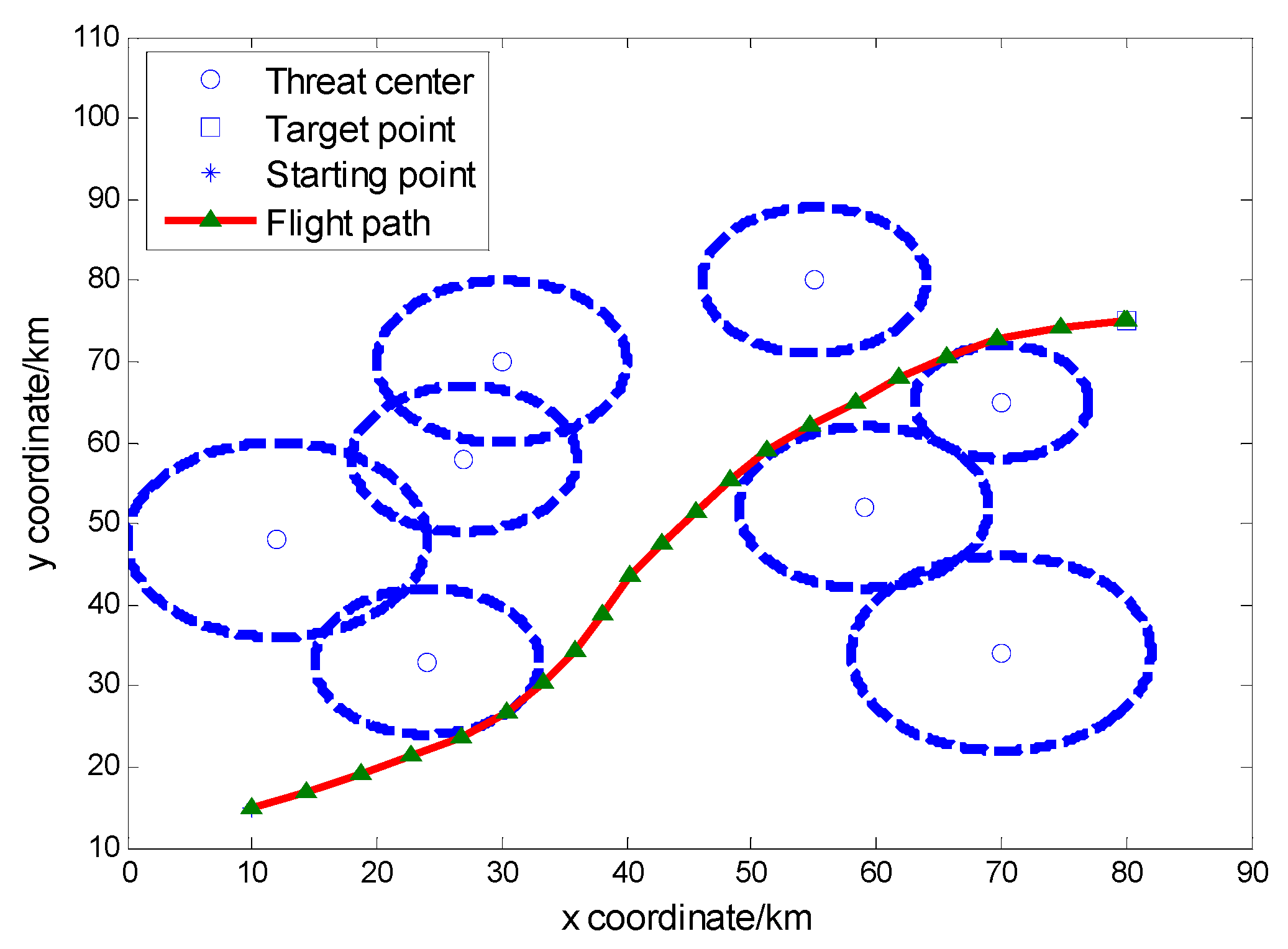
Table 12. Experimental results for the second test instance in different D.

Popsize	Maxgen	D	Result	DE	PSO	BA	WDO	QPSO	QBA	QWDO
30	200	5	Mean	108.4500391	76.32274731	217.8576809	158.6365421	58.55026343	224.8713213	86.06651884
			Best	51.51154424	51.51285958	51.62725599	53.3969487	51.52283974	51.56102341	51.51142514
			Worst	257.7693771	259.3727002	262.6262155	779.1292284	258.96214051	263.0166854	257.7692998
30	200	10	Mean	51.69531753	59.62698855	56.56107653	66.95686144	51.28710941	56.49182092	52.58309128
			Best	48.21839521	48.60012275	48.31096493	51.14078655	48.2522368	48.30357221	48.21752061
			Worst	60.65282489	71.23964789	63.92306031	102.9043651	61.60174489	66.80983521	60.56959953
30	200	15	Mean	50.073766	53.86901522	50.86134423	66.95568288	49.52489924	50.95870139	49.50373784
			Best	47.93535622	50.43482837	48.06959155	57.01360885	48.01888001	48.13432924	47.86853465
			Worst	51.57555205	59.96256435	52.76505672	74.82060029	51.6348462	56.00698594	50.82801702
30	200	20	Mean	49.84233544	51.48149235	50.90193378	66.66824246	49.67928022	50.07122862	48.81483482
			Best	48.12672661	49.24653359	48.16350755	58.430756	48.39737111	48.33316163	47.80715661
			Worst	52.11021304	54.24689277	67.44172011	75.96794054	51.30798995	53.42378109	49.74939729
30	200	25	Mean	50.66805474	50.95517305	51.34776811	71.70637996	50.83847029	50.60934221	48.59295541
			Best	48.70720514	49.54338148	48.79658763	59.14948465	48.75545861	48.39299019	47.83424938
			Worst	55.79533973	53.49953637	64.50598736	80.26246808	53.58558572	53.91518696	49.45543938

Table 12. Experimental results for the second test instance in different D.

Popsize	Maxgen	D	Result	DE	PSO	BA	WDO	QPSO	QBA	QWDO
30	200	5	Mean	108.4500391	76.32274731	217.8576809	158.6365421	58.55026343	224.8713213	86.06651884
			Best	51.51154424	51.51285958	51.62725599	53.3969487	51.52283974	51.56102341	51.51142514
			Worst	257.7693771	259.3727002	262.6262155	779.1292284	258.96214051	263.0166854	257.7692998
30	200	10	Mean	51.69531753	59.62698855	56.56107653	66.95686144	51.28710941	56.49182092	52.58309128
			Best	48.21839521	48.60012275	48.31096493	51.14078655	48.2522368	48.30357221	48.21752061
			Worst	60.65282489	71.23964789	63.92306031	102.9043651	61.60174489	66.80983521	60.56959953
30	200	15	Mean	50.073766	53.86901522	50.86134423	66.95568288	49.52489924	50.95870139	49.50373784
			Best	47.93535622	50.43482837	48.06959155	57.01360885	48.01888001	48.13432924	47.86853465
			Worst	51.57555205	59.96256435	52.76505672	74.82060029	51.6348462	56.00698594	50.82801702
30	200	20	Mean	49.84233544	51.48149235	50.90193378	66.66824246	49.67928022	50.07122862	48.81483482
			Best	48.12672661	49.24653359	48.16350755	58.430756	48.39737111	48.33316163	47.80715661
			Worst	52.11021304	54.24689277	67.44172011	75.96794054	51.30798995	53.42378109	49.74939729
30	200	25	Mean	50.66805474	50.95517305	51.34776811	71.70637996	50.83847029	50.60934221	48.59295541
			Best	48.70720514	49.54338148	48.79658763	59.14948465	48.75545861	48.39299019	47.83424938
			Worst	55.79533973	53.49953637	64.50598736	80.26246808	53.58558572	53.91518696	49.45543938

Table 13. Experimental results for the second test instance in different Maxgen.

Popsize	Maxgen	D	Result	DE	PSO	BA	WDO	QPSO	QBA	QWDO
30	50	20	Mean	60.11210553	52.10944247	54.69506882	75.33956531	54.98617763	53.48694368	50.04535423
			Best	54.63302708	49.63615429	49.15087344	64.96697732	51.63957205	49.77944089	48.06638554
			Worst	68.85463056	55.49586702	68.94866149	96.58202587	61.59178853	57.49410513	54.18169722
30	100	20	Mean	53.83836816	51.36653616	53.14143773	70.57187552	51.38397481	50.46414355	49.02122905
			Best	48.33976811	49.07513681	48.69510082	57.67068514	48.99505905	48.42088512	47.86003025
			Worst	60.13601866	53.46121189	75.25004292	83.08842351	55.59578695	54.24391665	50.15146747
30	150	20	Mean	51.05336892	51.57677078	50.84575891	70.54479972	50.45391734	50.39693696	48.72957492
			Best	49.40096571	49.67670378	48.62648502	62.80958025	48.41389406	48.52347097	47.82128972
			Worst	55.88497818	54.28141398	61.23851396	76.00858334	52.69768873	53.3014373	49.54581499
30	200	20	Mean	49.9035051	51.5013683	50.16504165	69.76739786	49.73289806	49.82207652	48.67284272
			Best	48.39387138	49.74179751	48.44930632	62.87834457	48.17837129	48.31338872	47.80987825
			Worst	50.94635705	54.31102253	61.2292916	76.48909998	51.56006612	52.70993366	49.85033671
30	250	20	Mean	49.6679397	51.96561739	50.3002217	67.90792328	49.25710679	49.76274007	48.78279719
			Best	47.94541607	50.42009286	48.23889332	60.92844125	48.12683235	48.16417909	47.80721825
			Worst	52.17249675	55.53271834	61.53309025	77.23621705	50.74799695	52.16236524	49.51742143

Table 13. Experimental results for the second test instance in different Maxgen.

Popsize	Maxgen	D	Result	DE	PSO	BA	WDO	QPSO	QBA	QWDO
30	50	20	Mean	60.11210553	52.10944247	54.69506882	75.33956531	54.98617763	53.48694368	50.04535423
			Best	54.63302708	49.63615429	49.15087344	64.96697732	51.63957205	49.77944089	48.06638554
			Worst	68.85463056	55.49586702	68.94866149	96.58202587	61.59178853	57.49410513	54.18169722
30	100	20	Mean	53.83836816	51.36653616	53.14143773	70.57187552	51.38397481	50.46414355	49.02122905
			Best	48.33976811	49.07513681	48.69510082	57.67068514	48.99505905	48.42088512	47.86003025
			Worst	60.13601866	53.46121189	75.25004292	83.08842351	55.59578695	54.24391665	50.15146747
30	150	20	Mean	51.05336892	51.57677078	50.84575891	70.54479972	50.45391734	50.39693696	48.72957492
			Best	49.40096571	49.67670378	48.62648502	62.80958025	48.41389406	48.52347097	47.82128972
			Worst	55.88497818	54.28141398	61.23851396	76.00858334	52.69768873	53.3014373	49.54581499
30	200	20	Mean	49.9035051	51.5013683	50.16504165	69.76739786	49.73289806	49.82207652	48.67284272
			Best	48.39387138	49.74179751	48.44930632	62.87834457	48.17837129	48.31338872	47.80987825
			Worst	50.94635705	54.31102253	61.2292916	76.48909998	51.56006612	52.70993366	49.85033671
30	250	20	Mean	49.6679397	51.96561739	50.3002217	67.90792328	49.25710679	49.76274007	48.78279719
			Best	47.94541607	50.42009286	48.23889332	60.92844125	48.12683235	48.16417909	47.80721825
			Worst	52.17249675	55.53271834	61.53309025	77.23621705	50.74799695	52.16236524	49.51742143

Figure 14. Result of the second instance for Maxgen = 100.

Figure 14. Result of the second instance for Maxgen = 100.

Figure 15. Result of the second instance for Maxgen = 150.

Figure 15. Result of the second instance for Maxgen = 150.

Figure 16. Result of the second instance for Maxgen = 200.

Figure 16. Result of the second instance for Maxgen = 200.

Figure 17. Result of the second instance for Maxgen = 250.

Figure 17. Result of the second instance for Maxgen = 250.

Figure 18. Fitness of the second instance for Maxgen = 50.

Figure 18. Fitness of the second instance for Maxgen = 50.

Figure 19. Fitness of the second instance for Maxgen = 100.

Figure 19. Fitness of the second instance for Maxgen = 100.

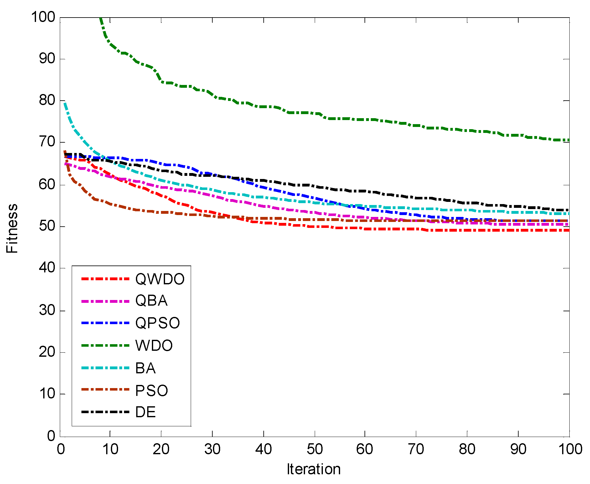
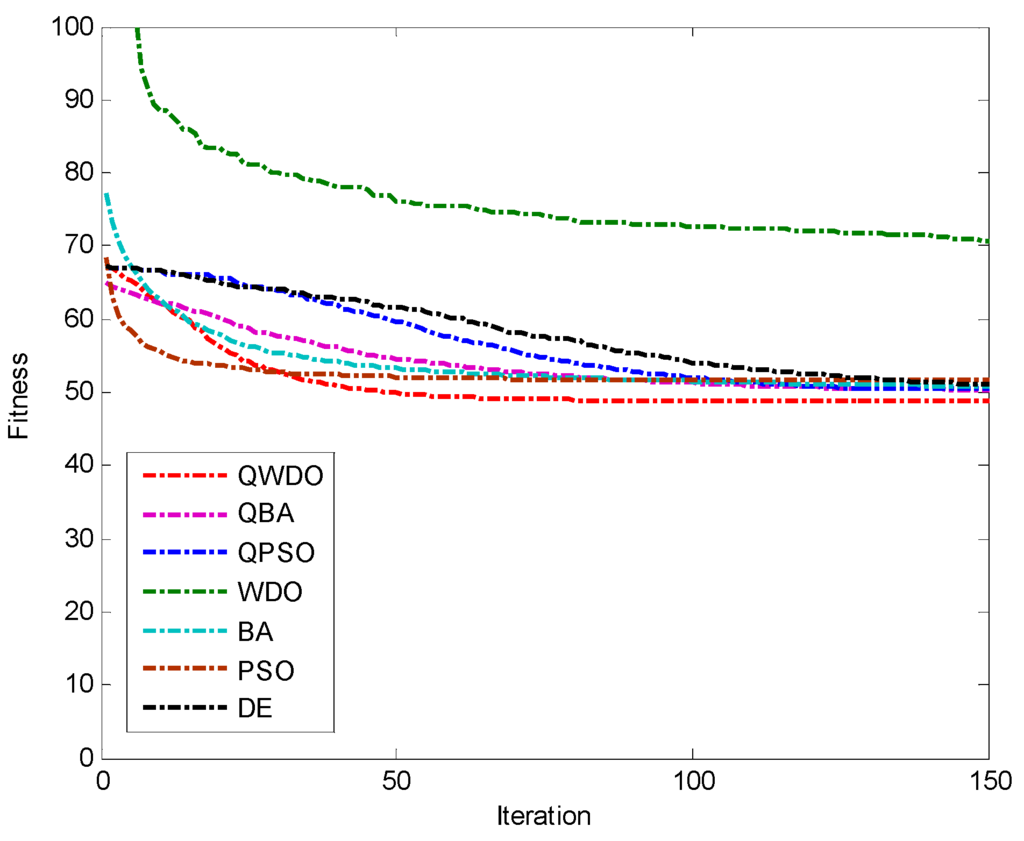
Figure 20. Fitness of the second instance for Maxgen = 150.

Figure 20. Fitness of the second instance for Maxgen = 150.

Figure 21. Fitness of the second instance for Maxgen = 200.

Figure 21. Fitness of the second instance for Maxgen = 200.

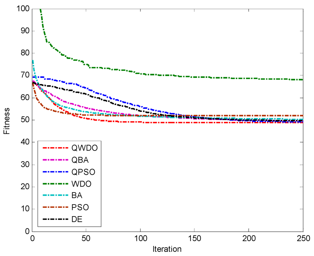
Figure 22. Fitness of the second instance for Maxgen = 250.

Figure 22. Fitness of the second instance for Maxgen = 250.

7. Conclusion and Future Research

In this paper, we present a new global optimization algorithm called quantum wind driven optimization (QWDO), which is based on the wind driven optimization (WDO) and quantum behavior for solving optimization problems. In order to evaluate the performance of the QWDO algorithm for solving the UCAV path-planning problem, we choose two test instances for testing. The simulation results show that the QWDO algorithm has a faster convergence rate and higher convergence precision in most cases. In comparison with QBA, QPSO, WDO, BA, PSO and DE algorithms, the QWDO algorithm is more effective in finding better solutions. QWDO is a reliable and feasible solution in solving the UCAV path-planning problem.

In this paper, the proposed QWDO algorithm was only implemented for the UCAV path-planning problem in two-dimensional space. Thus, our future work will concentrate on applying the QWDO algorithm in solving the UCAV path-planning problem in three-dimensional space. In the field of optimization, there are still many aspects worthy of study. In the future, we want to apply this algorithm to practical applications in other fields.

References

- Ma, Q.; Lei, X. Application of improved particle swarm optimization algorithm in UCAV path planning. Artif. Intell. Computat. Intell. 2009, 5855, 206–214. [Google Scholar]
- Ma, Q.; Lei, X. Application of artificial fish school algorithm in UCAV path planning. In Proceeding of the 2010 IEEE Fifth International Conference on Bio-Inspired Computing: Theories and Applications (BIC-TA), Changsha, China, 23–26 September 2010; pp. 555–559.
- Duan, H.B.; Zhang, X.Y.; Xu, C.F. Bio-Inspired Computing; Science Press: Beijing, China, 2011. [Google Scholar]
- Wang, G.; Guo, L.; Duan, H.; Liu, L.; Wang, H. A bat algorithm with mutation for UCAV path planning. Sci. World J. 2012, 2012. [Google Scholar] [CrossRef]
- Wang, G.; Guo, L.; Duan, H.; Liu, L.; Wang, H. A modified firefly algorithm for UCAV path planning. Int. J. Hybrid Inf. Technol. 2012, 5, 123–144. [Google Scholar]
- Li, B.; Gong, L.; Yang, W. An improved artificial bee colony algorithm based on balance-evolution strategy for unmanned combat aerial vehicle path planning. Sci. World J. 2014, 2014. [Google Scholar] [CrossRef] [PubMed]
- Zhou, Q.; Zhou, Y.; Chen, X. A Wolf Colony Search Algorithm Based on the Complex Method for Unmanned Combat Air Vehicle Path Planning. Int. J. Hybrid Inf. Technol. 2014, 7, 183–200. [Google Scholar] [CrossRef]
- Zhu, W.; Duan, H. Chaotic predator-prey biogeography-based optimization approach for UCAV path planning. Aerosp. Sci. Technol. 2014, 32, 153–161. [Google Scholar] [CrossRef]
- Bayraktar, Z.; Komurcu, M.; Werner, D.H. Wind Driven Optimization (WDO): A novel nature-inspired optimization algorithm and its application to electromagnetics. In Proceeding of the Antennas and Propagation Society International Symposium (APSURSI), Toronto, ON, Canada, 11–17 July 2010; pp. 1–4.
- Bayraktar, Z.; Komurcu, M.; Bossard, J.A.; Werner, D. The wind driven optimization technique and its application in electromagnetics. IEEE Trans. Antennas Propag. 2013, 61, 2745–2757. [Google Scholar] [CrossRef]
- Bhandari, A.K.; Singh, V.K.; Kumar, A.; Singh, G. Cuckoo search algorithm and wind driven optimization based study of satellite image segmentation for multilevel thresholding using Kapur’s entropy. Expert Syst. Appl. 2014, 41, 3538–3560. [Google Scholar] [CrossRef]
- Sun, J.; Wang, X.; Huang, M.; Gao, C. A Cloud Resource Allocation Scheme Based on Microeconomics and Wind Driven Optimization. In Proceeding of the 2013 8th Conference on ChinaGrid Annual Conference (ChinaGrid), Changchun, China, 22–23 August 2013; pp. 34–39.
- Boulesnane, A.; Meshoul, S. A new multi-region modified wind driven optimization algorithm with collision avoidance for dynamic environments. Adv. Swarm Intell. Springer Int. Publ. 2014, 8795, 412–421. [Google Scholar]
- Kuldeep, B.; Singh, V.K.; Kumar, A.; Singh, G.K. Design of two-channel filter bank using nature inspired optimization based fractional derivative constraints. ISA Trans. 2015, 54, 101–116. [Google Scholar] [CrossRef] [PubMed]
- Mahto, S.K.; Choubey, A.; Suman, S. Linear array synthesis with minimum side lobe level and null control using wind driven optimization. In proceeding of the 2015 International Conference on Signal Processing And Communication Engineering Systems (SPACES), Guntur, India, 2–3 January 2015; pp. 191–195.
- Yang, X.S. Nature-Inspired Optimization Algorithms; Elsevier: San Francisco, CA, USA, 2014. [Google Scholar]
- Li, S.Y.; Li, P.C. Quantum particle swarms algorithm for continuous space optimization. Chin. J. Quantum Electron. 2007, 24, 569–574. (In Chinese) [Google Scholar]
- Duan, H.; Li, P. Bio-Inspired Computation in Unmanned Aerial Vehicles; Springer Berlin Heidelberg: Berlin, Germany, 2014. [Google Scholar]
- Xu, C.; Duan, H.; Liu, F. Chaotic artificial bee colony approach to Unmanned Combat Air Vehicle (UCAV) path planning. Aerosp. Sci. Technol. 2010, 14, 535–541. [Google Scholar] [CrossRef]
- Li, P.; Duan, H.B. Path planning of unmanned aerial vehicle based on improved gravitational search algorithm. Sci. China Technol. Sci. 2012, 55, 2712–2719. [Google Scholar] [CrossRef]
- Riehl, H. Introduction to the Atmosphere; McGraw Hill: New York, NY, USA, 1978. [Google Scholar]
- Ahrens, C.D. Meteorology Today: An Introduction to Weather, Climate, and the Environment, 7th ed.; Thomson-Brook/Cole: Belmont, CA, USA, 2003. [Google Scholar]
- Hey, T. Quantum computing: An introduction. Comput. Control Eng. J. 1999, 10, 105–112. [Google Scholar] [CrossRef]
- Li, Z.Y.; Ma, L.; Zhang, H.Z. Quantum bat algorithm for function optimization. J. Syst. Manag. 2014, 21, 717–722. (In Chinese) [Google Scholar]
- Soares, J.; Silva, M.; Vale, Z.; de Moura Oliveira, P.B. Quantum-based PSO applied to hour-ahead scheduling in the context of smart grid management. In proceeding of the 2015 IEEE Eindhoven on PowerTech, Eindhoven, Dutch, 29 June–2 July 2015; pp. 1–6.
© 2015 by the authors; licensee MDPI, Basel, Switzerland. This article is an open access article distributed under the terms and conditions of the Creative Commons Attribution license (http://creativecommons.org/licenses/by/4.0/).