A Novel Classification Optimization Approach Integrating Class Adaptive MRF and Fuzzy Local Information for High Spatial Resolution Multispectral Imagery

Abstract

This paper develops a novel classification optimization approach integrating class adaptive Markov Random Field (MRF) and fuzzy local information (CAMRF-FLI) for high spatial resolution multispectral imagery (HSRMI). Firstly, the raw classification results, including initial fuzzy memberships and class labels of every pixel, are achieved by a pixel-wise classification method for a given image. Secondly, the class adaptive MRF-based data energy function is developed to integrate class spatial dependency information. Thirdly, a novel spatial energy function integrating fuzzy local information is constructed. Finally, based on the total of data and spatial energies, the raw classification map is regularized by a global minimization of the energy function using its iterated conditional modes (ICM). The effectiveness of CAMRF-FLI is performed by two data sets. The results indicate it can refine the classification map in homogeneous areas, meanwhile, reduce most of the edge blurring artifact, and improve the classification accuracy compared with some conventional approaches.

1. Introduction

Land cover information extracting from high spatial resolution multispectral imagery (HSRMI), such as WorldView, QuickBird, IKONOS image, etc., is an important remote sensing application. HSRMI can provide more detailed ground cover information. At the same time, increased spatial resolution always gives rise to spectral similarity, which in turn reduces the spectral statistical separability of different classes [1]. The conventional spectral pixel-wise classification methods, such as support vector machines (SVMs), maximum likelihood classifier (MLC), etc., are inadequate for HSRMI classification. While the abundant spatial information contained in the HSRMI may help for accurate classification. So a lot of spectral–spatial classification methods have been developed and proved to be successful in improving the classification accuracy [2].

Generally, two main strategies are utilized to include spatial information to the classification. One is preprocessing, in which the spatial information is exploited and combined in a feature vector of every pixel for the pixel-wise classification methods [3,4,5]. Another is the classification postprocessing (CPP), in which spatial dependences are considered in the decision rule [6,7,8,9]. In this paper, we focus on CPP algorithms. Several CPP methods have been investigated and confirmed effective in enhancing classification result [10]. Among them, the Majority voting (MV) filter is the simplest and most widely CPP method, in which the class of central pixel is classified as the majority class in a sliding window. Unfortunately, high accuracies are obtained at the cost of oversmooth losing image details [11]. Gaussian filter (GS) was proposed to improve MV, in which, the class of the central pixel is determined by weighted class fuzzy memberships based on the Gaussian distance in a local window [12]. However this method neglects the centered pixel’s own features. Thus, it may produce oversmoothed results. The object-based voting (OBV) method aims to refine the raw classification result by conducting the MV based on the boundary derived from the image segmentation [13]. However, the effectiveness of OBV depends on performance of segmentation. MRF is a classic CPP method, in which the raw classification map is smoothed through the dependence among neighboring pixels [14,15]. While the traditional MRF often leads to oversmoothed solutions for the equal weighted neighbor’ influences and fixed coefficient β. To overcome this defect, some enhanced MRF were proposed and proved to be effective in preserving image details to a certain extent [16,17,18]. These works had developed more complex spatial priori models to suppress the smoothness effect. And the models can effectively preserve boundaries. Unfortunately, these MRF models involving local discontinuities still exist unexpected and isolated class labels around object boundaries. Besides, the selection of the penalty coefficient β is difficult and time-consuming in these methods. From above discussion, we can find that most of CPP methods can obtain correct classification result in homogenous regions, while a lot of errors frequently occur on boundaries. A more efficient method should be developed to deal with such boundary pixels issues.

This paper presents a novel classification optimization approach integrating class adaptive Markov Random Field (MRF) and fuzzy local information (CAMRF-FLI) approach for HSRMI classification. The aim is to provide a proper trade-off between oversmooth and spatial regularization to produce homogeneous regions while preserving image details. The CAMRF-FLI is validated through two experiments. Results showed that the CAMRF-FLI was effective in improving classification accuracy.

2. Methodology

In this section, we first briefly introduce class adaptive MRF for integrating the class spatial dependency information. Then, a novel local similarity measure is developed to incorporate fuzzy local information. Last, the proposed approach is described in details.

2.1. Class Adaptive MRF

Considering an image $\mathbf{X}=\left\{{\mathit{x}}_1,{\mathit{x}}_2,\cdots {\mathit{x}}_i,\cdots ,{\mathit{x}}_n\right\}$, $x_i\in R_B$, represents a dataset in the B-dimensional vector space, $n$ is the number of pixels, and $c$ is the number of classes ($2\le c<n$) in the image.

The MRF is widely used to incorporate spatial contextual information into image classification by the dependence among neighboring pixels [10]. In which the prior probability serves as an operator for directly exploiting the contextual information. According to the Harmmersley–Clifford theorem and Gibbs theory [4], for pixel $x_i$, the prior probability is described as

$$P_k(x_i)=\frac{\exp (-\beta E_k(x_i))}{{\displaystyle \sum _{k^{\prime }=1}^c\exp (-\beta E_{k^{\prime }}(x_i))}}$$

(1)

where $\beta$ is a smoothing parameter that reflects the interaction between two neighboring pixels, $E_k(x_i)$ is the energy function of pixel $x_i$ belongs to the kth class, it is defined as

$$E_k(x_i)={\displaystyle \sum _{j\in N_i}(1-\delta (k(x_i),k(x_j))})$$

(2)

where $N_i$ is the neighbors of pixel $x_i$, $i\notin N_i$, often defined as a second order neighboring system (8-neighborhood connectivity) in the traditional MRF, $k(x_i)$ and $k(x_j)$ denotes the label of pixel $x_i$ and its neighboring pixel $x_j$, respectively. $\delta (k(x_i),k(x_j))$ is the Kronechker’s delta function.

$$\delta (k(x_i),k(x_j))=\{\begin{array}{cc}1& k(x_i)=k(x_j)\\ 0& \mathrm{otherwise}\end{array}$$

(3)

In the MRF, $\beta$ is a very important coefficient which controls the effect between two pixels, while its selection is difficult and time-consuming in practice. In the traditional MRF, equal influences are put on the central pixel $x_i$ from the neighboring pixels without considering the local image statistics characteristics and whether the neighboring pixel is an edge pixel or not. As a result, it performs well in homogeneous areas, while edge pixels are at the risk of oversmooth. Besides, $\beta$ is fixed for all neighbor windows for the whole image and the local image information may be overlooked. To address above problems, we propose a new class adaptive coefficient ${\beta }^{*}$.

$${\beta }^{*}=\frac{1}{N_R}\sqrt{{\displaystyle \sum _{j\in N_i}{(u_k(x_i)-u_k(x_j))}^2}}$$

(4)

where $N_R$ is its cardinality, $u_k(x_i)$ and $u_k(x_j)$ denotes the fuzzy memberships of pixels $x_i$ and $x_j$ belongs to the kth class, respectively. Based on the above-mentioned discussion, a novel prior probability function $P_k^{*}(x_i)$ is proposed as

$$P_k^{*}(x_i)=\frac{\exp (-{\beta }^{*}{E}_k(x_i))}{{\displaystyle \sum _{k^{\prime }=1}^c\exp (-{\beta }^{*}{E}_{k^{\prime }}(x_i))}}$$

(5)

here, the shape of local window ($N_i$) is square, but other shape windows can also be used, and the neighborhood size is not just only 8-neighborhood, other more big window size can also be used.

As seen from Equations (4) and (5), there are no experimental parameters. The determination of ${\beta }^{*}$ is based on fuzzy memberships differences between two pixels, and it is adaptive to classes and anisotropic in the neighborhood, which is consistent with the fact the image is anisotropic, thus it can preserve more details than using the fixed one.

2.2. A Novel Local Similarity Measure

In this paper, the local similarity measure comprises the spatial distance factor and the intensity distance factor. For one pixel, the spatial constraint reflects the damping extent of the neighbors by the distance from the central pixel and is represented as

$$w_{\mathrm{d}}=\frac{1}{d(x_i,x_j)}$$

(6)

here $x_i$ is the central pixel in the neighborhood $N_i$, and $x_j$ represents the neighbor of $x_i$. $d(x_i,x_j)$ represents the Euclidean distance between pixel $x_i$ and pixel $x_j$. Seen from Equation (6), we can find $w_{\mathrm{d}}$ is determined by the distance between the centered pixel and its neighbors, as a result, more local context information can be exploited.

But it is not enough to show the damping extent of the neighborhood by the distance alone. Here, the intensity distance is introduced to consider local grey level statistics. The intensity distance $w_{\mathrm{u}}(k)$ between two pixels is defined as

$$w_{\mathrm{u}}(k)=u_k(x_i)\times u_k(x_j)$$

(7)

From equation (7), we can find that the class similarity between two pixels is proportional to the $w_{\mathrm{u}}(k)$, a high value means that there is a high probability that the pixels $x_i$ and $x_j$ belong to the same class, and vice versa.

Therefore, the similarity measure $w_{ij}(k)$ between pixels $x_i$ and $x_j$ can be defined as

$$w_{ij}(k)=w_d\times w_u$$

(8)

Obviously, no experimental parameters are needed in the similarity measure, and the pixel is affected by its neighboring pixels and itself simultaneously, and the local similarity measure is also adaptive to classes and anisotropic in the neighborhood, which is useful for remaining boundary pixels and image details when performing spatial regularization.

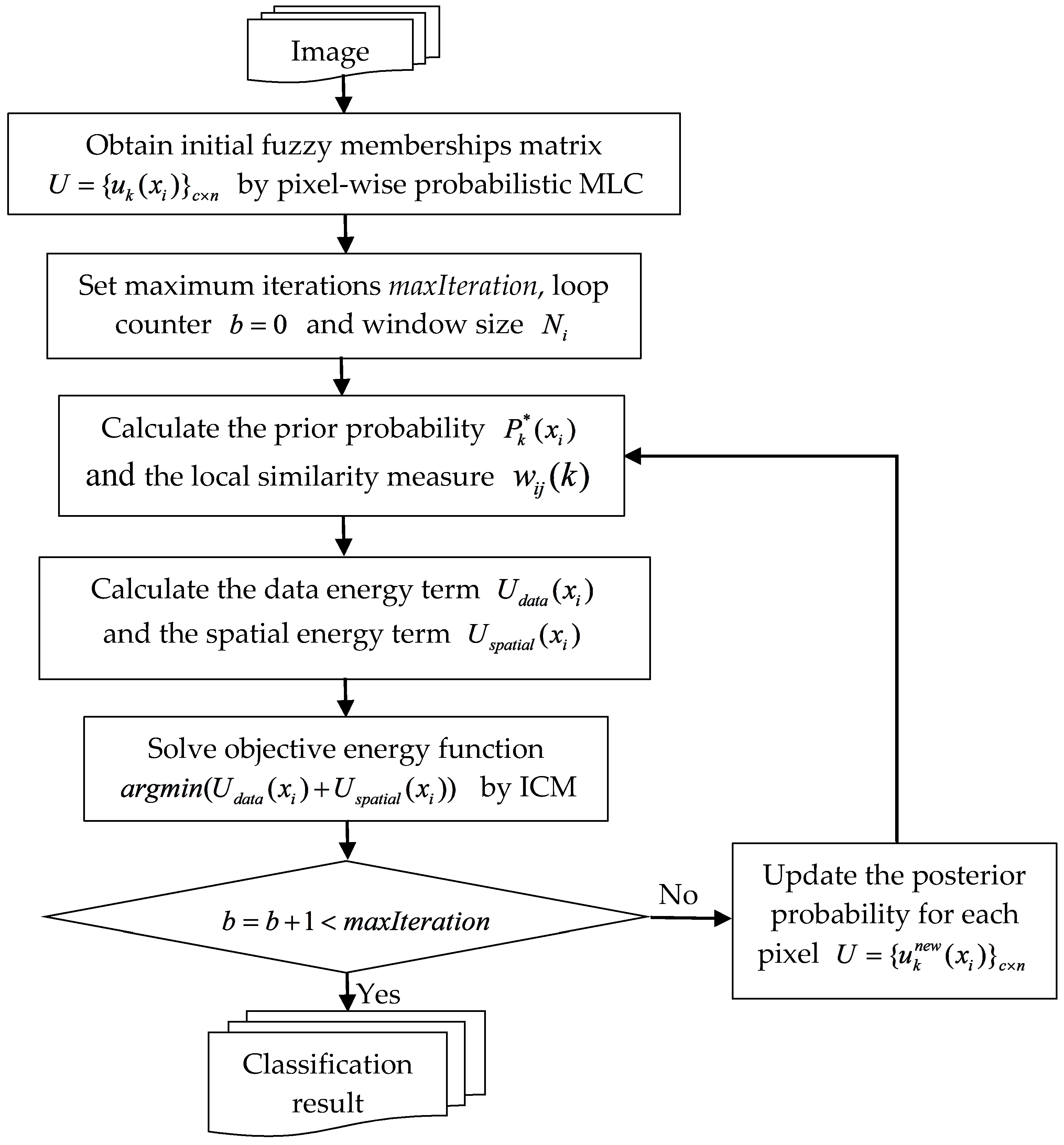
2.3. Proposed Method

Following the MRF-based image classification algorithm, the CAMRF-FLI is proposed by incorporating the prior probability function and local similarity measure. We perform the regularization of classification map in the MAP-MRF framework. The framework is based on the interpixel class dependence assumption that neighboring pixels tend to belong to the same class. Based on the Bayesian approach, an optimization is formulated as the minimization of the global objective energy in the image by iterative minimization of local energies. Details of the MRF-based classification approach have been introduced previously [10]. The local energy of function for a pixel $x_i$ is represented as

$$U(x_i)=U_{data}(x_i)+U_{spatial}(x_i)$$

(9)

where $U_{data}(x_i)$ is the data energy term, and $U_{spatial}(x_i)$ is the spatial energy term, in the CAMRF-FLI method, considering the class spatial dependency information, by incorporating the prior probability function describe in Equation (5), the data energy function is defined as

$$U_{data}(x_i)=-\ln (u_k(x_i)\times P_k^{*}(x_i))$$

(10)

And considering the class spatial dependency information, by introducing the local similarity measurement described in Equation (8), in the CAMRF-FLI method, the spatial energy term is defined as

$$U_{spatial}(x_i)=-\ln ({\displaystyle \sum _{j\in N_i}{u}_k(x_j)\times w_{ij}(k)})$$

(11)

To minimize the energy function Equation (9), many algorithms have been proposed, such as Simulated Annealing (SA), Maximum a Posterior Margin (MPM), ICM, etc. [4]. Considering computational simplicity, Equation (9) is solved by the ICM method, in addition, at each iteration in the ICM, the fuzzy memberships for each pixel are updated by

$$u_k^{new}(x_i)={\displaystyle \sum _{k^{\prime }=1}^c\left(\frac{u_k(x_i)\times P_k^{*}(x_i)+{\displaystyle \sum _{j\in N_i}{u}_k(x_j)\times w_{ij}(k)}}{u_{k^{\prime }}(x_i)\times P_{k^{\prime }}^{*}(x_i)+{\displaystyle \sum _{j\in N_i}{u}_{k^{\prime }}(x_j)\times w_{ij}(k^{\prime })}}\right)}$$

(12)

The flowchart of proposed CAMRF-FLI approach is shown in Figure 1. The implementation includes the following five steps:

Step 1:

Initialization

The initial fuzzy memberships matrix $U={\{u_k(x_i)\}}_{c\times n}$ is obtained by the pixel-wise probabilistic MLC method, set maximum iterations as maxIteration, loop counter $b=0$ and window size $N_i$

Step 2:

Calculate the prior probability $P_k^{*}(x_i)$ and the local similarity measure $w_{ij}(k)$

$P_k^{*}(x_i)$ and $w_{ij}(k)$ are calculated according to Equations (5) and (8), respectively.

Step 3:

Calculate the data energy term $U_{data}(x_i)$ and the spatial energy term $U_{spatial}(x_i)$

Based on the calculated $P_k^{*}(x_i)$ and $w_{ij}(k)$, $U_{data}(x_i)$ and $U_{spatial}(x_i)$ are calculated according to Equations (10) and (11), respectively.

Step 4:

Solve objective energy function

The objective energy $U(x_i)=U_{data}(x_i)+U_{spatial}(x_i)$ is minimized by the ICM algorithm.

Step 5:

Termination

The iteration will stop when $b=b+1<maxIteration$ is met; otherwise, update the posterior probability for each pixel $U={\{u_k^{new}(x_i)\}}_{c\times n}$ according to Equations (12), and go back to Step 2 and repeat.

The main contributions of CAMRF-FLI are as follows. (1) It is free of any experimentally adjusted parameters. (2) The class spatial dependency information is considered by introducing the class adaptive MRF-based prior probability function. (3) The spectral dissimilarity is taken into account by incorporating the local similarity measurement based fuzzy local information. The identification of centered pixel is determined by the spatial dependency and spectral information of its own and neighbors’ pixels simultaneously, to a certain extent the CAMRF-FLI approach can refine the classification map in homogeneous areas and reduce the boundary pixels classification errors simultaneously.

3. Experimental Results and Discussion

In order to assess the effectiveness of the proposed algorithm, performances of CAMRF-FLI are analyzed and compared with MLC, MV, MRF, OBV, and GS methods through two experiments. In the two experiments, the parameter β for MRF is set as 1, and the iteration is set at 100 for MRF and CAMRF-FLI. For OBV method, eCognition 8.9 software is used to obtain the segmentation map, and the related parameters are scale = 10, wcolor = 0.3. The window sizes for MV, GS, and CAMRF-FLI are changed from 3 × 3 to 19 × 19. The study areas cover grass, water, building, tree, bare soil, road, and shadow. The reference image is acquired by visual interpretation based on the well rectified image, 20% of the reference data is used as the train samples through the stratified random sampling method, and the remainder of the reference data is used as the testing samples. All algorithms were developed in Matlab 2013b. The Producer’s Accuracy, Overall Accuracy (OA), and Kappa coefficient (κ) (based on the confusion matrix) are used to evaluate the classification performance. Considering computational simplicity, MLC is applied to obtain the posterior probability and initial class label for every pixel in experiments. Each algorithm is run ten times and the average classification accuracy, and the optimal classification results are derived.

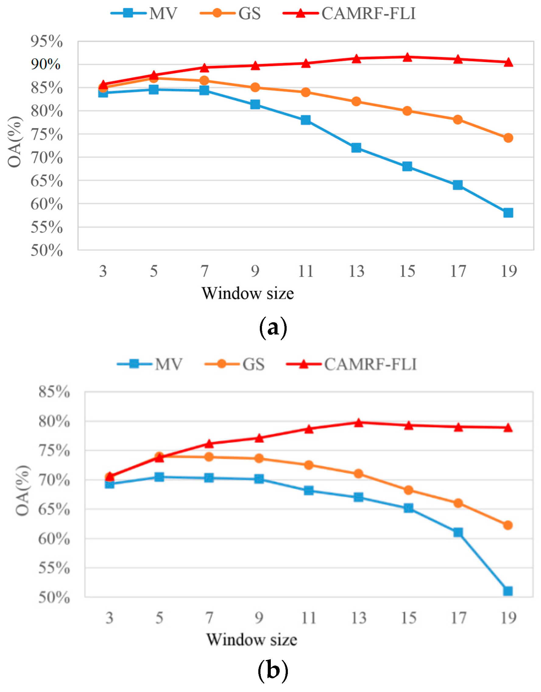
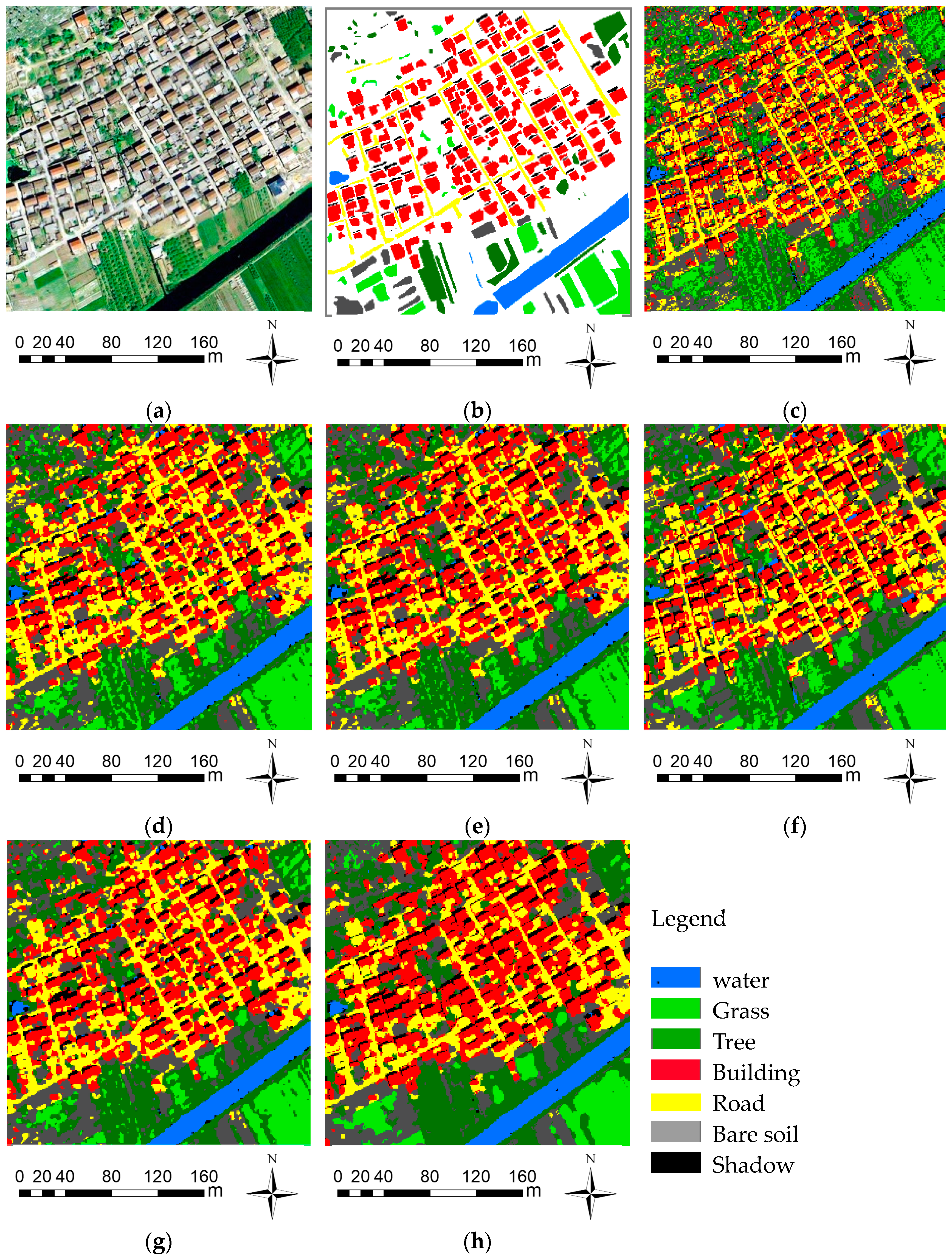
3.1. Experiment on Data Set 1

In this experiment, a portion of a 0.61-m resolution QuickBird (512 × 512 pixels) image including three multispectral bands (red, green, and blue), which was obtained on August, 2005 (Figure 2a), is used. The study area locates in an urban area in Xuzhou City, China. Figure 2b shows the reference image.

Table 1. Number of samples, producer’s accuracy, OA, and κ of the classification in experiment 1.

Class	Training Samples	Testing Samples	MLC	MV (5 × 5)	MRF	OBV	GS (5 × 5)	CAMRF-FLI (15 × 15)
Water	2010	8042	91.93%	96.53%	95.47%	97.28%	96.12%	95.93%
Grass	1047	4187	78.43%	81.01%	77.02%	79.27%	76.84%	81.59%
Tree	1355	5421	53.22%	53.02%	68.48%	62.39%	72.20%	93.65%
Building	7846	31,383	52.52%	55.51%	57.74%	54.50%	58.76%	91.13%
Road	1863	7454	86.73%	91.89%	89.70%	92.54%	90.30%	86.09%
Bare soil	1130	4522	80.09%	86.15%	87.78%	90.15%	89.34%	98.41%
Shadow	1134	4536	70.84%	82.95%	88.60%	96.13%	89.75%	96.19%
OA			80.79%	84.61%	86.11%	85.16%	87.15%	91.60%
κ			0.7494	0.7949	0.8145	0.8028	0.8278	0.8852

describes the training and testing samples in the experiment 1. From Figure 2a, we can find the distributions of road and building are irregular and complex, the spectral similarity between road and building is high, and the same situation for water and shadow, grass and tree, etc., it is difficult to classify the image only using spectral information.

Figure 3a gives the OA curves obtained with different window sizes for MV, GS, and CAMRF-FLI algorithms tested in Experiment 1, respectively. They have similar OA with small window size, while CAMRF-FLI provides a significant advantage over MV and GS in terms of OA with the increase of window size. MV and GS obtain the highest OA with a 5 × 5 window, and CAMRF-FLI has the highest OA with a 15 × 15 window. Figure 2c–h shows the classification results deriving from the MLC, MV (5 × 5), MRF, OBV, GS (5 × 5), and CAMRF-FLI (15 × 15), respectively. As shown in Figure 2c, because many mixed or spectral similar pixels exist, MLC shows a map with “salt and pepper” without incorporating spatial contextual information. Figure 2d–h all give more homogenous regions than MLC, but GS and CAMRF-FLI are more effective in eliminating isolated pixels. GS removes almost of the isolated pixels and obtains satisfactory results, but oversmooth results occur on boundaries and producing large patches. In the CAMRF-FLI results, most of the isolated pixels are eliminated and image details are satisfactorily remained. Seen from Table 1, CAMRF-FLI produces the highest OA and most of the best Producer’s Accuracies. The OA gains of CAMRF-FLI over MLC, MV, MRF, OBV, and GS are 10.81%, 6.99%, 5.49%, 6.44%, and 4.45%, respectively; the classification accuracies are statistically significant at the 5% level of significance.

3.2. Experiment on Data Set 2

In this experiment, a QuickBird image (512 × 512 pixels) including three 0.61-m resolution fused multispectral bands (red, green, and blue) is applied. It locates the suburb area of Xuzhou, China, which was obtained on August, 2005 (Figure 4a). As shown in Figure 4a, the spectral information between road and building is very similar, and the same situation for water and shadow, grass, tree, etc. The road and building staggers distribution, thus, it is difficult to classify the image with spectral information alone. Figure 4b gives the reference image.

Table 2. Number of samples, producer’s accuracy, OA, and κ of the classification in experiment 2.

Class	Training Samples	Testing Samples	MLC	MV (5 × 5)	MRF	OBV	GS (5 × 5)	CAMRF-FLI (13 × 13)
Water	2042	8167	92.49%	96.77%	95.91%	97.55%	96.69%	97.60%
Grass	2468	9874	80.46%	80.86%	77.16%	83.40%	77.08%	80.67%
Tree	2075	8302	52.30%	53.24%	68.94%	59.03%	73.16%	90.35%
Building	9087	36,347	53.47%	56.90%	58.96%	56.53%	60.19%	67.77%
Road	2435	9741	86.30%	91.35%	89.03%	89.84%	89.47%	84.80%
Bare soil	1089	4354	79.28%	85.88%	87.21%	90.86%	89.25%	97.24%
Shadow	982	3930	69.44%	77.86%	85.55%	90.31%	86.31%	98.83%
OA			66.86%	70.23%	72.40%	71.74%	73.66%	79.75%
κ			0.5900	0.6299	0.6558	0.6495	0.6706	0.7419

shows the training and testing samples in the experiment 2.

As shown in Figure 3b, MV, GS, and CAMRF-FLI algorithms also have similar OA with small window size, but CAMRF-FLI shows more robust to the window size than MV and GS in terms of OA. Seen from Figure 3b, MV and GS obtain the highest OA at the 5 × 5 window, and CAMRF-FLI achieves the best OA at the 13 × 13 window. Figure 4c–h shows the classification results provided by MLC, MV (5 × 5), MRF, OBV, GS (5 × 5), and CAMRF-FLI (13 × 13) algorithms, respectively. In Figure 4c, for the spectral similarity, MLC obtains a map with “salt and pepper” noise without incorporating spatial information, road and building and bare soil, tree and grass, and water and shadow are confused in the classification result. Figure 4d–h all obtain more homogenous regions than Figure 4c for incorporating spatial information, while MV, MRF, OBV, and GS show weaker performance than CAMRF-FLI. CAMRF-FLI produces homogeneous areas while preserving more image details. Table 2 gives the quantitative results. In Table 2, MV, MRF, OBV, GS, and CAMRF-FLI achieve higher classification accuracies than MLC. Among them, CAMRF-FLI obtains the highest OA and most of the best Producer’s Accuracies. In terms of OA, CAMRF-FLI achieves a value of 79.75%, with gain of 12.89%, 9.52%, 7.35%, 8.01%, and 6.09% over other algorithms, respectively. According to the results of McNemar’s test, all classification accuracies are statistically significant at the 5% level of significance.

Based on quantitative and qualitative assessments, CAMRF-FLI achieves the best performance for most classes. The reason for this may be that MLC utilizes spectral alone in the classification, thus producing poor results for mixed or spectral similar pixels. For the other methods, MV simply assigns the majority class in a sliding window to the centered pixel without considering different effects on the central pixel from its neighborhood, as a result, high OA is obtained at the cost of oversmooth. The result of OBV mainly depends on the performance of segmentation, while a fine segment result is difficult to obtain, usually producing large patches and removing details. In GS, Gaussian distance function is used to describe different weights on the centered pixel, but the class spatial dependency information between neighboring pixels is not considered, and also neglecting the centered pixel’s own features. Thus, it may produce oversmoothed results. MRF applies the spatial regularization by utilizing neighbor label information to produce homogeneous areas, while neighboring pixels’ influences on the centered pixel are treated equally, β is fixed for all neighbor windows across the whole image, and only 8-neighborhood is considered. As a result, in the homogeneous areas, the classification is enhanced, while some classification errors often happened on the edges of the regions. In contrast, CAMRF-FLI introduces the class spatial dependency information and the local similarity measure based fuzzy local information, thus, it can provide a good trade-off between oversmooth and spatial regularization and, hence, reduces the edge blurring artifacts and preserves small patches when performing spatial regularization.

4. Conclusions

A novel CAMRF-FLI approach for HSRMI classification has been presented in the paper. The proposed method is effective in refining classification map in homogeneous areas and preserving more details simultaneously. The advantage is due to the introduced class spatial dependency information and local similarity measure based fuzzy local information, which can provide a good trade-off between oversmooth and spatial regularization. Two different experiments were used to test the performance of CAMRF-FLI, and compared with MV, OBV, MRF, and GS it obtains the best performance both visually and quantitatively for most classes. Hence, CAMRF-FLI is an effective optimization approach for HSRMI classification.

In next studies, more study will be carried on methods of optimizing the energy function, and the proposed algorithm will be tested on other remote sensing images, etc.

References

1. Fauvel, M.; Tarabalka, Y.; Benediktsson, J.A.; Chanussot, J.; Tilton, J.C. Advances in spectral-spatial classification of hyperspectral Images. Proc. IEEE 2012, 101, 652–675. [Google Scholar] [CrossRef]
2. Huang, X.; Zhang, L. An SVM ensemble approach combining spectral, structural, and semantic features for the classification of high-resolution remotely sensed imagery. IEEE Trans. Geosci. Remote Sens. 2013, 51, 257–272. [Google Scholar] [CrossRef]
3. Huang, X.; Lu, Q.; Zhang, L.; Plaza, A. New postprocessing methods for remote sensing image classification: A systematic study. IEEE Trans. Geosci. Remote Sens. 2014, 11, 7140–7159. [Google Scholar] [CrossRef]
4. Li, S. Markov Random Field Modeling in Image Analysis; Springer: New York, NY, USA, 2010. [Google Scholar]
5. Lu, Q.; Huang, X.; Liu, T.; Zhang, L. A structural similarity-based label-smoothing algorithm for the post-processing of land-cover classification. Remote Sens. Lett. 2016, 7, 437–445. [Google Scholar] [CrossRef]
6. Moser, G.; Sebastiano, B.; Serpico, S.; Benediktsson, J. Land-cover mapping by markov modeling of spatial–contextual information in very-high-resolution remote sensing images. Proc. IEEE 2013, 101, 631–651. [Google Scholar] [CrossRef]
7. Myint, S.W.; Gober, P.; Brazel, A.; Grossman-Clarke, S.; Weng, Q. Per-pixel vs. object-based classification of urban land cover extraction using high spatial resolution imagery. Remote Sens. Environ. 2011, 115, 1145–1161. [Google Scholar] [CrossRef]
8. Schindler, K. An overview and comparison of smooth labeling methods for land-cover classification. IEEE Trans. Geosci. Remote Sens. 2012, 50, 4534–4545. [Google Scholar] [CrossRef]
9. Tarabalka, Y.; Fauvel, M.; Chanussot, J. SVM- and MRF-based method for accurate classification of hyperspectral images. IEEE Geosci. Remote Sens. Lett. 2010, 7, 736–740. [Google Scholar] [CrossRef]
10. Wang, L.; Huang, X.; Zheng, C.; Zhang, Y. A Markov random field integrating spectral dissimilarity and class co-occurrence dependency for remote sensing image classification optimization. ISPRS J. Photogramm. Remote Sens. 2017, 128, 223–239. [Google Scholar] [CrossRef]
11. Zhang, H.; Shi, W.; Wang, Y.; Hao, M.; Miao, Z. Classification of very high spatial resolution imagery based on a new pixel shape feature set. IEEE Geosci. Remote Sens. Lett. 2014, 11, 940–944. [Google Scholar] [CrossRef]
12. Aghighi, H.; Trinder, J.; Tarabalka, Y.; Samsung, L. Dynamic block-basedparameter estimation for MRF classification of high-resolution images. IEEE Geosci. Remote Sens. Lett. 2014, 11, 1687–1691. [Google Scholar] [CrossRef]
13. Büschenfeld, T.; Ostermann, J. Edge preserving land cover classification refinement using mean shift segmentation. In Proceedings of the 4th International Conference on GEographic Object Based Image Analysis, Rio De Janeiro, Brazil, 7–9 May 2012; pp. 242–247. [Google Scholar]
14. Foody, G.M. Thematic map comparison: Evaluating the statistical significance of differences in classification accuracy. Photogramm. Eng. Remote Sens. 2004, 70, 627–633. [Google Scholar] [CrossRef]
15. Kang, X.D.; Li, S.T.; Jon Atli Benediktsson, J.A. Spectral–spatial hyperspectral image classification with edge-preserving filtering. IEEE Trans. Geosci. Remote Sens. 2014, 52, 2666–2677. [Google Scholar] [CrossRef]
16. Zhang, H.; Bruzzone, L.; Shi, W.Z.; Hao, M. Enhanced spatially constrained remotely sensed imagery classification using a fuzzy local double neighborhood information c-means clustering algorithm. IEEE J. Sel. Top. Appl. Earth Obs. Remote Sens. 2018, 11, 2896–2910. [Google Scholar] [CrossRef]
17. Yu, Q.; Clausi, D.A. IRGS: Image segmentation using edge penalties and region growing. IEEE Trans. Pattern Anal. Mach. Intell. 2008, 30, 2126–2139. [Google Scholar] [PubMed]
18. Zhang, G.; Jia, X. Simplified conditional random fields with class boundary constraint for spectral-spatial based remote sensing image classification. IEEE Geosci. Remote Sens. Lett. 2012, 9, 856–858. [Google Scholar] [CrossRef]
Figure 1. Flowchart of the proposed CAMRF-FLI method.
Applsci 08 01792 g001
Figure 2. Dataset and classification results in Experiment 1. (a) QuickBird image of Xuzhou RGB (red, green, blue), center coordinates: [34°10′18.61″ N, 117°12′23.44″ E]. (b) Reference data. (ch) is the classification result using MLC, MV (5 × 5), MRF, OBV, GS (5 × 5), and CAMRF-FLI (15 × 15), respectively.
Applsci 08 01792 g002aApplsci 08 01792 g002b
Figure 3. (a,b) shows the OA obtained with different window sizes for MV, GS, and CAMRF-FLI algorithms tested in experiments 1 and 2, respectively.
Applsci 08 01792 g003
Figure 4. Dataset and classification results in Experiment 2. (a) QuickBird image of Xuzhou RGB (red, green, blue), center coordinates: [34°12′45.80″ N, 117°05′6.94″ E]. (b) Reference data. (ch) is the classification result using MLC, MV (5 × 5), MRF, OBV, GS (5 × 5), and CAMRF-FLI (13 × 13), respectively.
Applsci 08 01792 g004