1. Introduction
With the availability of distributed generation (DG) and energy storage systems (ESSs), the application of advanced information communication and power electronics technologies, and the utilization of demand-side resources, the traditional distribution network is gradually developing into a multicoordinated active distribution network (ADN) [
1]. The important feature of the ADN is openness and interaction. Compared with the past, the power sources, networks, and demand-side loads in the ADN have changed greatly and have strong flexibility. With the cooperation of flexible power sources, the predictability and controllability of various intermittent renewable energy sources have been greatly improved. In terms of loads, flexible loads are increasingly becoming the trend of load development. By combining controllable conventional loads with various energy storage components and demand-side response means, increasing regulation demand of the power system can be adapted. The development of information technology has also facilitated the exchange of information between the source, network, and loads and has enhanced the interactions among the three. In addition, access to various power electronic devices also enhances the controllability of the power grid. All of these new changes provide convenient conditions for the coordinated operation of the source–network–load of the ADN, making it an important development trend in the future.
Measurement devices, communication equipment, and control systems make up the essential backbone of ADN operation. In order to ensure reliable operation of the ADN and effective control of the source–network–load, first it is necessary to ensure reliable monitoring and communication of DGs and ESSs. Reference [
2] proposes a new solution for the remote monitoring and control of DGs and ESSs connected to distribution networks with the function of voltage regulation and power shuttering. Reference [
3] develops a new interface device solution and a proper communication architecture, which allows implementing remote control of DG power production or islanding detection. Reference [
4] proposes a new method considering power lines as an alternative communication medium for remote monitoring applications of smart grids for renewable energy sources. Second, the network side can realize the monitoring, control, and fast fault isolation of a distribution network by means of automated distribution technology. One way to achieve distribution automation is by implementing substation automation systems [
5]. For the demand-side resources, communication technologies such as advanced metering infrastructure (AMI) and supervisory control and data acquisition (SCADA) can acquire the user-side information in time, so as to formulate the corresponding incentive scheme and actively manage the user-side load, which ensures the smooth implementation of demand-side management and demand response [
6].
In view of the optimal scheduling problem of the ADN, relevant research has been carried out from different angles. Aiming at the uncertainties of wind turbine (WT) and photovoltaic (PV) cell output, an energy-optimal scheduling model for an ADN with WTs, PV cells, and ESSs is proposed based on chance constrained programming in reference [
7]. In reference [
8], the optimal scheduling operation of an ADN is considered. However, the optimization object is limited to the active and reactive “source” of the ADN and does not involve flexible topology adjustment of the network and flexible load control. To be part of the network reconfiguration, distributed generation and distribution network reconfiguration are optimized together to minimize total power loss and improve the voltage stability index in [
9].
As user-side resources gradually participate in the demand response (DR), researchers began to study demand response models. The main purpose of the DR is to minimize customers’ electricity payment [
10] or achieve a generally uniform electricity load profile [
11]. During the scheduling process of the ADN, demand response is always applied in combination with DG control. The source-load coordinated optimization scheduling in the distribution network mainly includes minimizing system operation costs [
12], improving the utilization ratio of renewable energy and user satisfaction [
13], smoothing renewable energy outputs [
14], reducing renewable generation curtailment [
15], and selecting the site and size of DGs for the purpose of coordinating multiple interests [
16,
17]. Reference [
18] focuses on the optimal intraday scheduling of a distribution system that includes renewable energy generation, energy storage systems, and thermostatically controlled loads. Reference [
19] proposes a multiobjective dynamic economic scheduling model considering the EVs and uncertainties of wind power to minimize the total fuel cost and pollutant emissions. Reference [
20] uses multiscene technology to deal with the uncertainty of intermittent DGs and loads, and a two-step optimal scheduling model of ADN considering day-ahead and real time is established. Reference [
21] proposes a multi-timescale cost-effective power management algorithm for islanded microgrid operation targeting generation, storage, and demand management. However, in our study, the DR is implemented with responsive loads that consider the uncertainty of the load participation. Moreover, the satisfaction of users participating in the demand response is modeled.
With the gradual application of ESSs, the management of demand-side loads also becomes possible [
22]. In Reference [
23], to minimize the cost of power loss, robust optimization is used to deal with the uncertainty of electricity price and the day-ahead scheduling problem of ESSs and responsive loads. Reference [
24] comprehensively considers a variety of adjustable resources in the ADN, such as DGs, ESSs, voltage regulators, switchable capacitor banks, and interruptible loads, to minimize the total operating cost of the system in the scheduling cycle. To reduce curtailment from renewable distributed generation, reference [
25] chooses minimum storage sizes at multiple locations in distribution networks. Considering the space-time relationship between ESSs and flexible loads as well as the influence of power flow, a multiobjective ADN optimization scheduling model is constructed in reference [
26], and the synergy is quantified by setting the priority of the scheduling units of each generation unit.
When it comes to research on optimal scheduling of source–network–load coordination, the single objective of the system operating cost is mainly considered. In order to realize the optimal control of DGs, networks, and demand-side loads, a smart distribution network optimization model with the minimum operating cost is proposed in reference [
27]. Reference [
28] proposes a comprehensive operational scheduling model to determine optimal decisions on active elements of the network, DGs, and responsive loads, seeking to minimize the day-ahead composite economic cost. Reference [
29] presents a mixed-integer dynamic optimization model for the optimal scheduling of ADNs with the objective of minimizing the daily costs of electricity purchased from distribution substations. Reference [
30] develops a framework for operational scheduling of distribution systems with dynamic reconfiguration considering coordinated integration of energy storage systems and demand response programs to minimize the total costs, including cost of total loss, switching cost, cost of bilateral contract with power generation owners and responsive loads, and cost of exchanging power with the wholesale market. Reference [
31] introduces a multiagent system and multilayer electricity price response mechanism to construct an optimization model of the distribution network layer, direct coordination source–load layer, and indirect coordination microgrid layer. Reference [
32] proposes an optimal scheduling model aiming to find the lowest operating cost of a complete scheduling period, and taking controllable DGs and tie switches as control means. The impact of electricity price and the adjustment of tie switches on the operating cost is considered, and the energy conservation and capacity constraints of the ESSs throughout the scheduling period are guaranteed. Reference [
33] proposes a source–network–load coordinated economic scheduling method in an ADN considering the electricity purchase cost, power loss cost, and demand-side management cost and taking DGs, ESSs, flexible network topologies, interruptible loads, and transferable loads as the control means.
To summarize, in the present research on optimal ADN scheduling, there are mainly the following problems:
The abundant controllable resources and diverse scheduling means are not fully considered, which is mainly limited to some aspect of source–network–load, such as the source–load interaction.
The scheduling model tends to aim for economic optimization while ignoring the uncertainty of WTs, PV cells, and loads.
The scheduling model has only one objective and fails to fully consider the interaction between the source–network–load, which cannot guarantee that multiple aspects will be simultaneously optimal.
This paper comprehensively utilizes the controllable elements of DGs, ESSs, switches, and interruptible loads in the ADN, fully considers the uncertainties of renewable energy and demand-side load response, and establishes a multiobjective scheduling model with coordinated source–network–load, which aims at finding the lowest operating cost, the highest renewable energy utilization rate, and the highest user satisfaction in the scheduling cycle. The NSGA3 algorithm is used to solve the three-objective scheduling model, and the performance of the algorithm is compared with another algorithm. The main contributions of the paper include the following:
Considering the deficiency of control measures for existing scheduling strategies, the proposed method fully considers the controllable resources of the source–network–load, including the DGs, switches, responsive loads, and storage systems. The specific control method includes DG control, network reconfiguration, and demand-side management.
Different from previous single-objective models, a three-objective scheduling model with coordinated source–network–load is proposed, considering the lowest operating cost, the highest renewable energy utilization rate, and the highest user satisfaction
Different from the method of transforming three objectives into one single objective by weight coefficients, this paper uses the NSGA3 algorithm to calculate the Pareto solution set of the optimization model and uses a fuzzy decision-making method to filter the solution set.
The remainder of this work is organized as follows. In
Section 2, we propose the scheduling strategy of source–network–load in the ADN. In
Section 3, we analyze the uncertainty of scheduling in the ADN. In
Section 4, we establish the multiobjective optimization scheduling model of the ADN. In
Section 5, we introduce the reference point–based many-objective evolutionary algorithm (NSGA3). Results are presented in
Section 6, and conclusions are drawn in
Section 7.
2. Scheduling Strategy of Source–Network–Load in the ADN
The ADN has a source–network–load ternary structure: “source” refers to all kinds of DGs and ESSs in the ADN, with DGs divided into controllable and intermittent types. Common controllable DGs include microturbines (MTs), diesel generators, fuel cells, etc., and intermittent DGs include WTs, PV cells, etc.; the “network” mainly includes transformers, lines, switches, and other power equipment, whose important function is to manage the power flow through a flexible network topology; “load” refers to various types of load resources on the demand side, including conventional loads, interruptible loads, etc. The control elements of ADN optimization scheduling in this paper include controllable DGs, ESSs, switches, and load resources. From the perspective of source–network–load, the ADN is a distribution system that can coordinate various types of DGs and ESSs, optimize the power flow based on the flexible topology, actively manage demand-side resources, promote the absorption of renewable energy generation, and ensure the safe and economic operation of the distribution network on the basis of meeting users’ electricity demands.
The specific scheduling strategy is shown in
Figure 1. The ADN dispatching center uses the corresponding communication devices to collect information of source–network–load three-terminal equipment and then figures out the corresponding dispatching scheme based on the proposed strategy. Finally, the control system controls the three source–network–load aspects to achieve the scheduling goals.
5. Solving Strategy Based on NSGA3
The above model is a nonlinear, multiperiod, and multiobjective optimization problem. In a multiobjective optimization problem, the relationship between optimal solutions is usually nondominated, and there are a few cases where one optimal solution dominates all other feasible solutions. Therefore, the optimal solution of the optimization problem is usually a set of solutions, called the nondominated solution set or the Pareto optimal solution set.
In the two-objective optimization problem, the nondominated sorting genetic algorithm 2 (NSGA2) with the crowding distance strategy is usually adopted [
42,
43,
44]. However, in the face of multiobjective optimization problems of three or more objectives, if we continue to use the crowding distance of NSGA2, the convergence and diversity of the algorithm will be problematic, such as an uneven distribution of the Pareto solution on the nondominated layer, resulting in the algorithm falling into a local optimum. Therefore, the reference point–based many-objective evolutionary algorithm (NSGA3) is proposed. The framework of the NSGA3 is basically the same as that of the NSGA2, except that the selection mechanism is different. The NSGA2 uses crowding distances to select individuals with the same nondominated level, while the NSGA3 uses a reference point–based approach [
45,
46] to select individuals.
5.1. The Basic Process of NSGA3
NSGA3 randomly generates the initial population containing N individuals, and then starts to iterate. In the tth generation, the algorithm generates the offspring population Qt by random selection, simulated binary crossover (SBX), and polynomial variation on the basis of the current population Pt. Both Pt and Qt are N in size. Then the two populations Pt and Qt are combined to form a new population Rt with a population size of 2N.
5.1.1. Population Classification into Nondominated Levels
In order to select the best N solutions from population Rt into the next generation, Rt is first divided into several different nondomination levels using a nondominated sorting method. Then, a new population St is constructed by adding the solutions of each nondomination level to St from level 1 until the size of St is equal to or greater than N for the first time. Assuming that the last acceptable nondomination level is level L, the solutions in level L + 1 are discarded, and the solution FL in level L is selected as the solution in the next population Pt+1. The remaining individuals in Pt+1 need to be selected from FL.
In the original NSGA2, a solution with a large crowding distance in FL is preferentially selected. However, the crowding distance is not suitable for solving multiobjective optimization problems of three or more objectives. Therefore, the NSGA3 no longer uses the crowding distance but adopts a new selection mechanism, which analyzes the individuals in St more systematically through the provided reference points and selects partial solutions in FL into Pt+1.
5.1.2. Reference Point Determination on a Hyperplane
The reference points of NSGA3 are critical, and the number of generated reference points depends on the dimension
m of the object vector and another positive integer
H.
The number of solutions of the equation can be calculated as follows:
Assume that
is the
jth solution of the equation, then reference point
λj can be obtained by Equation (27):
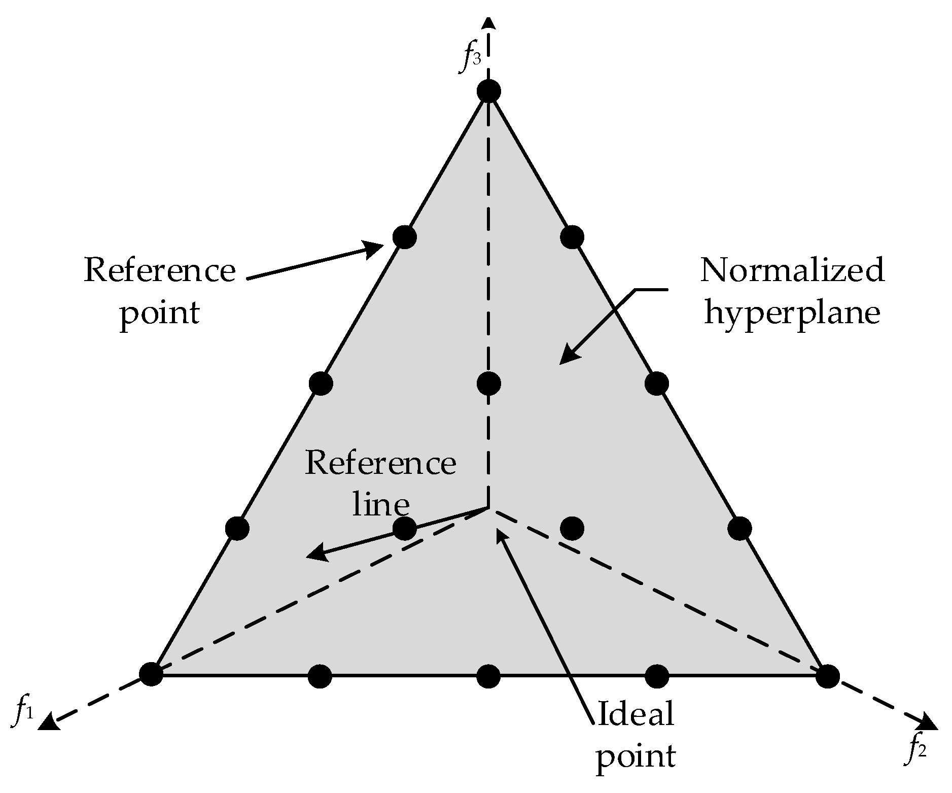
Geometrically speaking, reference points
are all located in the hyperplane, as shown in
Figure 3, and
H is the number of divisions along each objective axis.
5.1.3. Population Adaptive Normalization
First, the minimum value of each dimension i of M objective functions needs to be calculated. Assume that the acquired corresponding minimum value on the ith objective is zi, and the set of zi is the ideal point set mentioned in the NSGA3 algorithm.
Then use Equation (28) to translate objectives:
To find the extreme points, the achievement scalarizing function (ASF) as Equation (29) is used:
where
and satisfies that if
,
, else
; for
, a small value of 10
−6 is used to replace it.
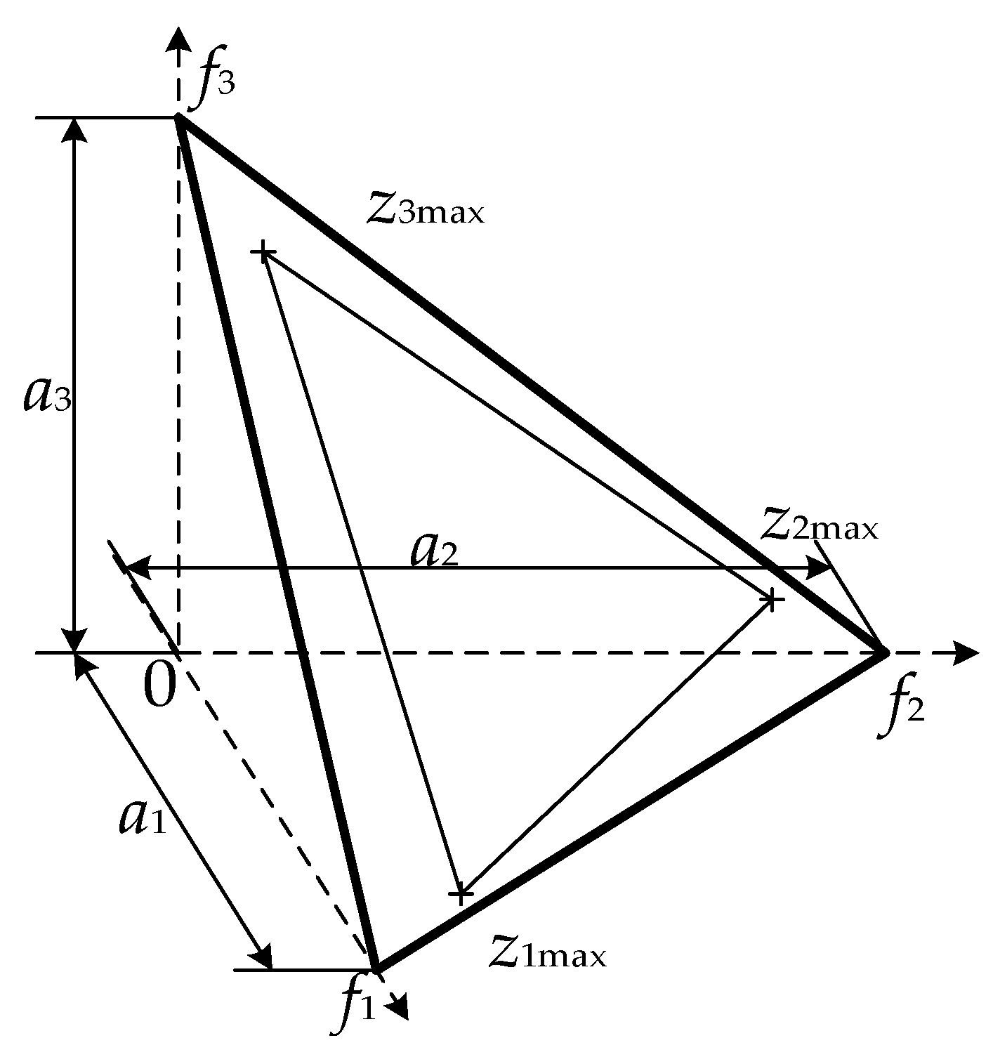
Traverse each function to find the individuals with the lowest ASF values, which are extreme points. These points and the origin (the ideal point) consist of three lines, which can form a hyperplane, as shown in
Figure 4. The intersections
between this surface and the three axes are the final intercepts. After finding the intercepts, normalization is carried out through Equation (30):
5.1.4. Association Operation
After normalization, the individuals need to be associated with the reference points. Use the line formed by the reference point and the origin as the reference line. For each individual, traverse all reference lines to find the nearest reference line to each population individual and record the information of the corresponding reference point and the shortest distance. The distance from the individual population to the reference line will be described by the perpendicular distance.
As shown in
Figure 5, suppose
u is the projection of
f(
x) on reference line L,
dj,1(
x) is the distance between the origin and
u, and
dj,2(
x) is the perpendicular distance from
f(
x) to line L. The distance can be calculated as follows [
47]:
After the association, each reference point will have the individual number ρj associated with it.
5.1.5. Niche-Preservation Operation
A reference point may have one or more population individuals associated with it or no individual population associated with it. Denote the niche count as ρj for the jth reference point and select the reference point j with minimum ρj.
If ρj = 0, this indicates that there are no solutions in the current population associated with this reference point. If there is a solution from the nondomination level that has the smallest distance to reference point j, the solution will be selected. Otherwise, the reference point is removed from the current population.
If ρj > 1, a solution associated with the reference point from the nondomination level will be randomly selected to add to the population.
5.1.6. Genetic Operations to Create Offspring Population
In NSGA3, after Pt+1 is formed, the offspring population Qt+1 is created by randomly selecting the parents from Pt+1 using conventional genetic operators (crossover and mutation).
5.1.7. Selection of Optimal Compromise Solution
In this paper, the fuzzy decision method [
48] is used to select the optimal compromise solution from the Pareto optimal solution set. The membership function
uij of the
jth objective value of the
ith Pareto solution
fij is:
For the
ith Pareto solution, its normalized membership function
ui is:
5.2. Probabilistic Power Flow Based on Monte Carlo Sampling
The power flow calculation is the basis for the optimization analysis of the ADN in this paper; due to the probability property of renewable energy and the load response, the power flow is uncertain. To deal with the problem, probabilistic power flow based on Monte Carlo sampling is used.
Use Monte Carlo sampling to generate lots of deterministic scenarios based on the probability distribution characteristics and the limits of renewable distributed power generation and controllable load response. Assume the number of sampling times is set to
k times. The random vectors of each controllable load and renewable power supply are obtained as Equation (34):
A large number of random sampling samples are obtained under certain constraints, and then deterministic power flow calculation is carried out to obtain the probability characteristics of the node voltage and branch power flow.
The estimation probability is expressed by the large number theorem; that is, the chance constraint condition, such as (17) and (18), holds if and only if the probability condition is satisfied.
Assume the number that satisfies the chance constraint condition is k’. The more Monte Carlo simulation scenarios are generated, the closer the estimated probability k’/k is to the probability that the actual chance constraints are satisfied.
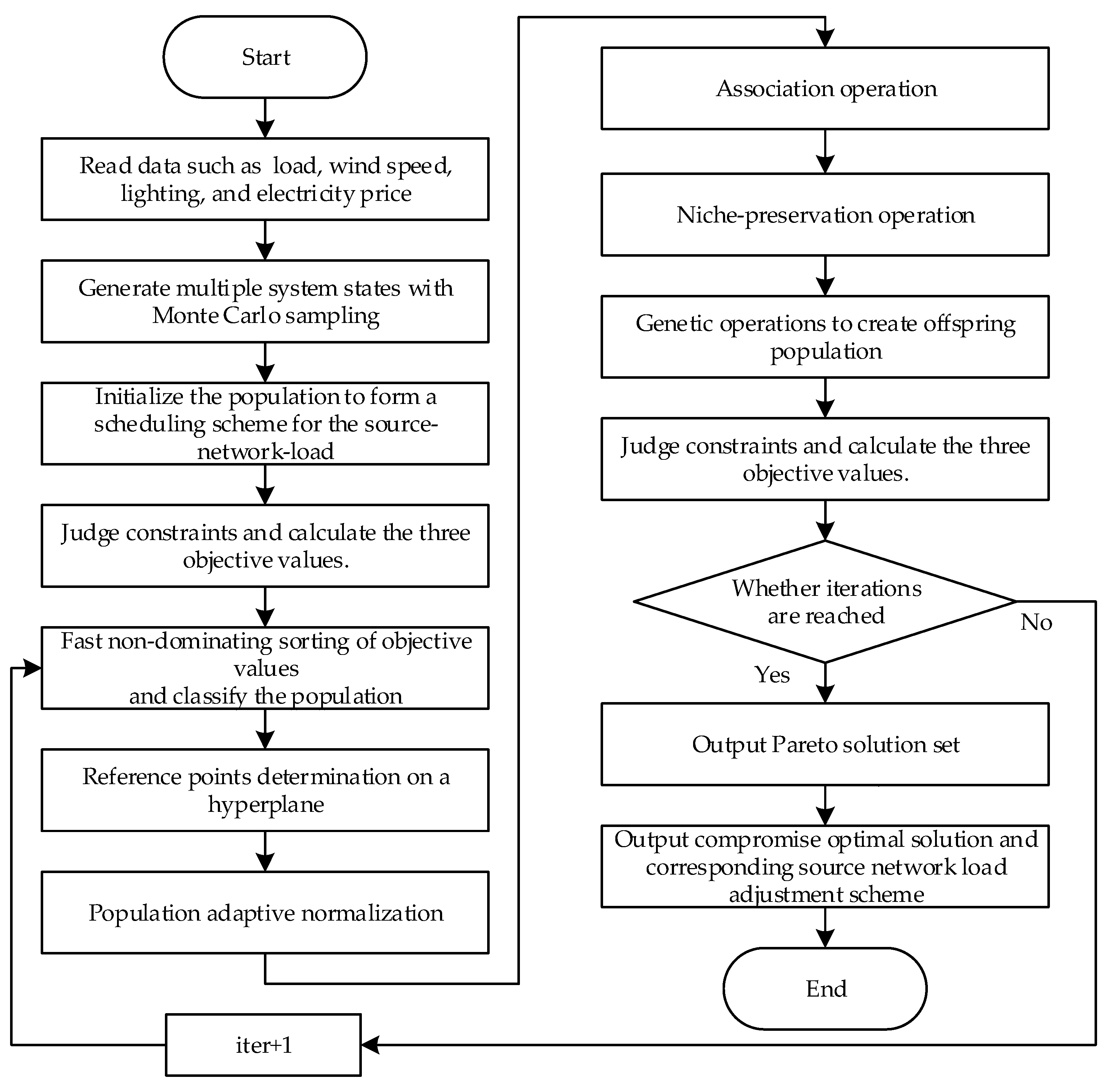
A flowchart of multiobjective optimal scheduling of the ADN based on the NSGA3 algorithm is shown in
Figure 6.
6. Discussion
The modified IEEE 33-bus distribution system as shown in
Figure 7 is used in this paper to carry out the analysis. Assume the loads from buses 22 to 32 will participate in demand-side management, which can reduce the load ratio by 10%, and the schedulable time is from 08:00 to 20:00. Two PV cells of 500 kW are installed at buses 9 and 17. Two WTs of 600 kW are installed at buses 4 and 32. Two MTs of 500 kW are installed at buses 8 and 15. Two 500 kW ESSs are installed at 17 and 32, whose SOC is 5%–95% [
49]. Assume the on-grid price of WTs is 0.30 CNY/kWh, the on-grid price of PV cells is 0.50 CNY/kWh, and the on-grid price of MTs is 0.40 CNY/kWh. Other specific parameters are shown in
Table A1. The time-of-use price and daily forecasting curve of loads, WTs, and PV cells are shown in
Figure 8 [
50].
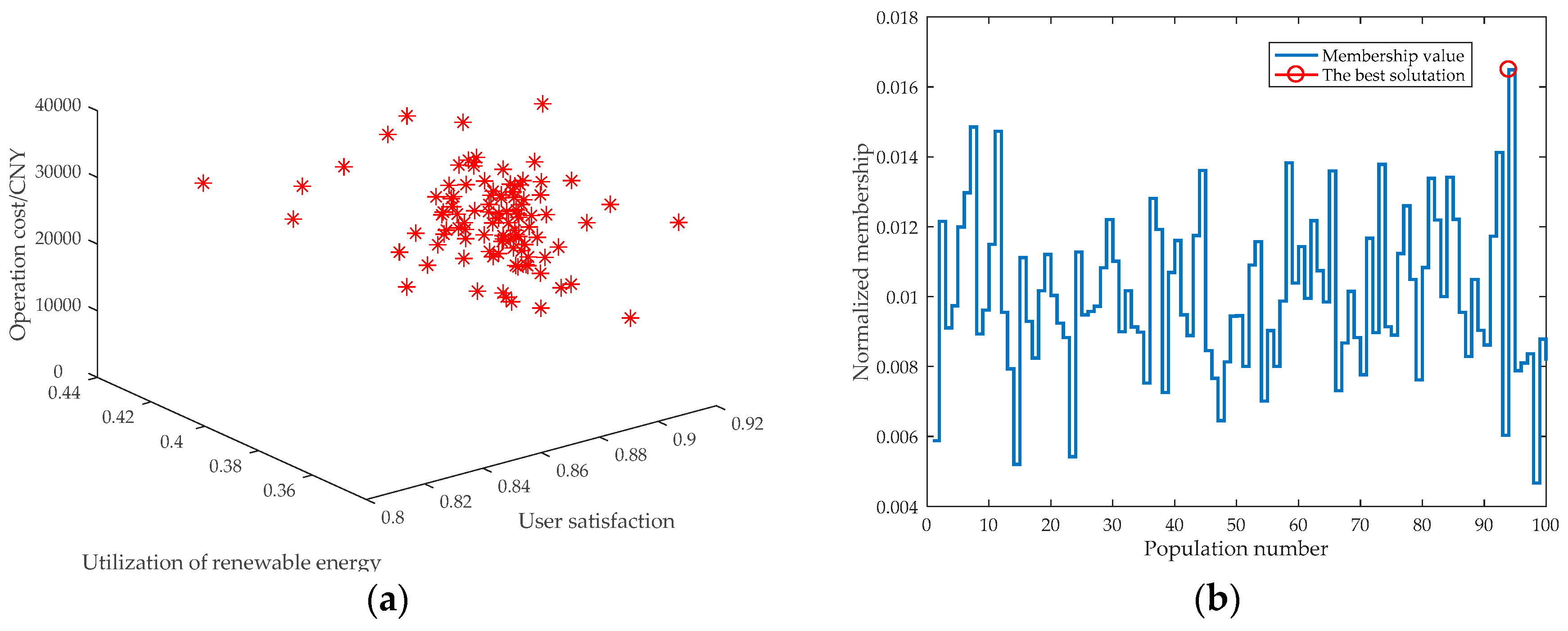
To reveal the coordination role of the source network load in the scheduling, the Pareto front solution set is simulated and analyzed according to the scheduling model proposed in this paper. The solution set is shown in
Figure 9, which consists of optimal solutions. In practice, the decision-makers can choose the final best solution according to the specific expectations of the distribution network. In this paper, the fuzzy decision method is used to analyze the optimization results. The solution with the largest membership function value is chosen as the final best solution, as shown in
Figure 9. This solution contains not only the information of the decision variables including the DG output power, the switch number, and the incentive price for the responsive load but also the information of objective values. The corresponding operating cost is 36811.14 CNY, the renewable energy utilization rate is 0.3909, and the user satisfaction is 0.8917.
The active power output plan of the MT and ESSs of the best solution is shown in
Figure 10. ESS1 is the energy storage of the PV bus and ESS2 is the energy storage of the WT bus. The MT is used when the load is heavy. On the one hand, the local power supply can reduce the power loss; on the other hand, it can save the electricity purchase cost during the peak period of high electricity price. The charge and discharge scheduling plans of ESSs are those that are charging during the daytime when the renewable DGs output is large, discharging at the peak of high electricity price in the evening, and charging at the low electricity price valley in the early morning. In this way, the ESS can smooth the fluctuation of renewable DG sources, clip peaks and fill valleys, and provide strong support for the economic and safe operation of the ADN.
The daily plan for load reduction and network topology adjustment is shown in
Table A2. Load reduction will bring additional demand-side management costs, so the scheduling plan only performs a small amount of load reduction at peak electricity prices. The flexible topology of the ADN is beneficial to reduce network loss, improve voltage quality, and reduce system uncertainty.
Figure 11 depicts the voltage uncertainty range of the network at various times. It can be seen from the figure that after adopting the optimized scheduling scheme, the voltage level of all periods is within the acceptable range and the uncertain range is acceptable.
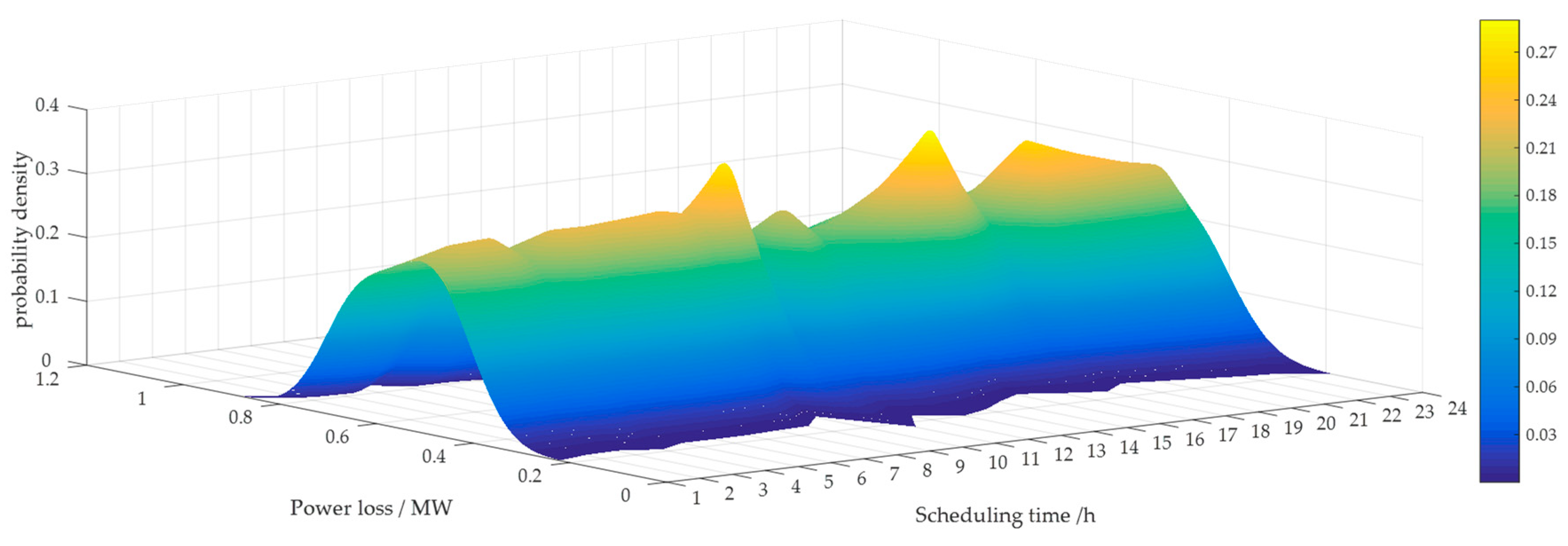
Figure 12 shows the probability density curve of power loss under the influence of uncertainty for 24 hours in the ADN. It can be seen that through source–network–load scheduling, power loss is at a lower level in a day and fluctuation is small.
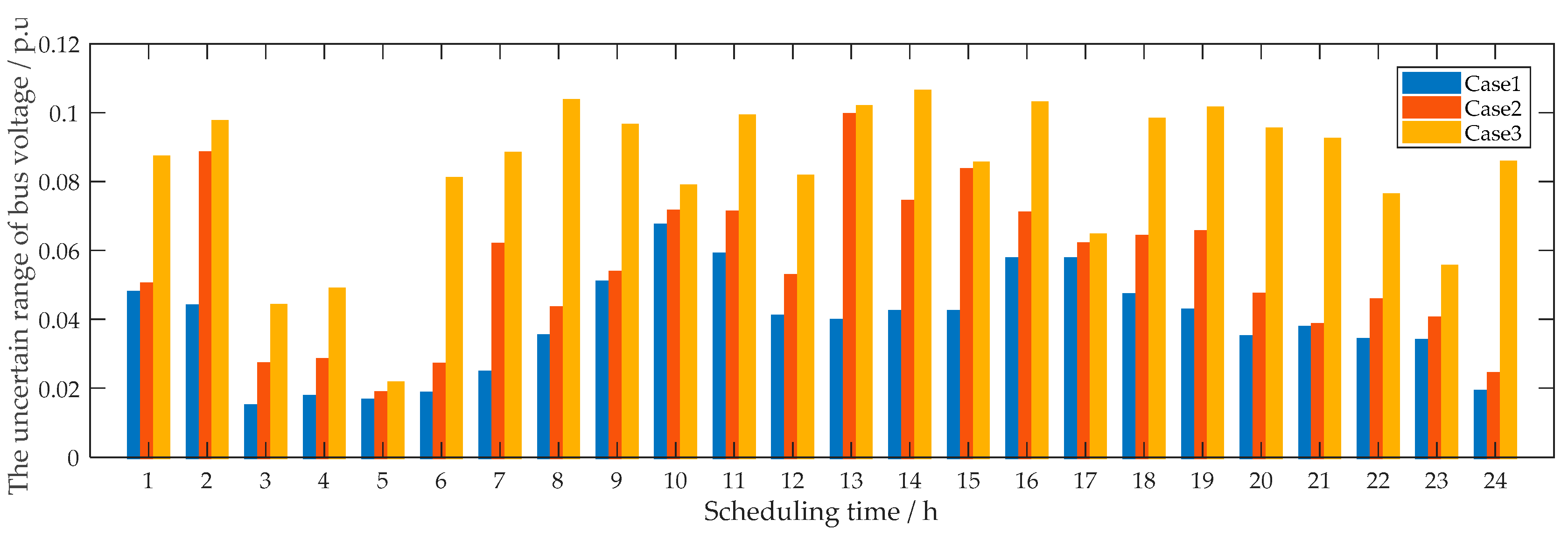
To reveal the coordinated role of source–network–load control in ADN scheduling, the following three scenarios in
Table 1 are simulated and analyzed according to the proposed scheduling model. The obtained objective function values are listed in
Table 2. The optimization results are contrasted from three aspects: minimum bus voltage, bus voltage uncertain range, and maximum power loss, shown in
Figure 13,
Figure 14 and
Figure 15.
From
Table 2, the operating cost of case 1 is the lowest due to the reasonable source–network–load scheduling. In case 2, the source–load control will require more controllable DGs and responsive load to participate in scheduling, thus reducing renewable energy utilization and user satisfaction. In case 3, no source–network–load control will lead to a high operating cost, and without the management of DGs and demand-side loads, renewable energy utilization will be at a high level and user satisfaction will not be affected.
Moreover, it can be seen from the results that in cases 2 and 3, when the load is heavy, there will be a certain risk of voltage violation, such as at 13:00, and the source–network load scheduling scheme significantly improves this phenomenon. In addition, the voltage uncertainty range of case 1 is also lower than the other two cases. Moreover, the total power loss of case 1 is reduced by 30.72% compared with case 3 and by 16.80% compared with case 2. On the whole, under the condition of coordinated scheduling of source–network–load, the minimum voltage profile, the range of voltage uncertainty, and the maximum power loss in 24 hours have advantages over the other two cases, which shows that the operation state of the active distribution network can be effectively improved by coordinated control of the source–network–load, and it also shows the effectiveness of the proposed method.
The effectiveness of the algorithm is verified by comparing it with NSGA2. By calculating the above example, a compromise optimal solution can be obtained by the fuzzy decision method, and the corresponding voltage variation can be acquired, as shown in
Table 3 and
Figure 16. The results show that the reference point–based NSGA3 algorithm performs better than the crowding distance–based NSGA2 when dealing with the three-objective optimization model.


