Abstract
Configuration techniques have been used in several fields, such as the design of business process models. Sometimes these models depend on the data dependencies, being easier to describe what has to be done instead of how. Configuration models enable to use a declarative representation of business processes, deciding the most appropriate work-flow in each case. Unfortunately, data dependencies among the activities and how they can affect the correct execution of the process, has been overlooked in the declarative specifications and configurable systems found in the literature. In order to find the best process configuration for optimizing the execution time of processes according to data dependencies, we propose the use of Constraint Programming paradigm with the aim of obtaining an adaptable imperative model in function of the data dependencies of the activities described declarative.
1. Introduction
A business process, henceforth referred to as BP, consists of a set of activities that are executed in coordination within an organizational and technical environment. These activities jointly attain a business goal [1]. Several languages propose an imperative representation of business processes, whose specification allows business experts to describe an explicit order of execution between activities, and to transform the process into an executable model (for example, that activities A, B and C are executed sequentially, or activities D and E are executed in parallel) [2,3,4,5,6]. Sometimes the order of the activities is therefore derived from the data dependencies, since these dependencies allow different configurations. In those cases, the imperative languages fail in the consideration of the data dependencies between activities. Configurable work-flows permit to include a degree of freedom about how the activities are related according to their data dependencies.
Configurable models tend to use a declarative representation of the configurable aspects. Although the imperative process models are significantly more understandable than declarative models [7,8], it is sometimes very difficult or even impossible to describe a problem in an imperative way [9,10]. One of the cases in business processes, where this difficulty can be found, is when the data relation can determine different activities order. The variation of the model is the reason several authors have proposed languages for the definition of BPs as declarative models [11,12,13,14]. Unfortunately, the data dependencies and its relation with declarative description has not been faced up.
This paper develops two ideas: (1) propose a declarative description of the activities that form a BP, including the data dependencies between them; (2) based on this declarative model, the declarative BP is automatically transformed into an imperative model where the work-flow is defined to minimize the execution time of the instances when the process is executed, and keeping the data dependencies relations. To obtain the imperative model, we propose the use of Constraint Programming, an Artificial Intelligence technique.
The analysis of the data interchanged during the process execution can affect to two aspects to optimize a BP: (i) attainment of a better business product, for example, by reducing the costs or satisfying customers’ preferences; and, (ii) the reduction of the execution time of the instances. The problem of determining the best product in terms of the input and output data of the activities is presented in [15]. In these studies only the first type of aspect is solved, specifically, the way in which the input data can influence the successful execution of a process is analyzed in order to find an optimized product. On the other hand, in the proposal presented in this paper, these previous works are extended to include the second aspect, the optimization of the execution of the instances regarding the data dependencies. How to order the activities by considering these data dependencies in an imperative representation is a hard and difficult task. It is a hard task because it requires an exhaustive analysis of the data dependencies, and it is a difficult task because the graphical representation of the process is not simple, being able to become a “spaghetti” process [16]. To support business experts in the design task, we propose an automatic transformation from the declarative model into an optimal imperative model where the execution time is minimized. The main reason of transforming declarative model into an imperative model is that imperative models are easier to implement in commercial Business Process Management Systems (BPMS).
Therefore, the aim of this article is to present a framework capable of obtaining the model configuration of the imperative description from a declarative specification based on data dependencies using Constraint Programming. This configurable system must also be able to detect errors and omissions in the declarative model, and to reason and validate the models through the different stages of the transformations. To the best of our knowledge, there are no proposals of declarative specification focused on data management, that create optimal executable BP using techniques of configuration.
The rest of the paper is organized as follows: Section 2 presents the example used in the paper to set out the proposal. Section 3 describes related work. Section 4 presents the Conf-BP Framework. Each individual component of the framework is then described in detail. Section 4.1 formalizes the declarative specification and applies it to the example. Section 4.2 proposes the automatic transformation of the declarative configurable model into a imperative BP. Section 4.3 defines the configurable system in charge of the transformation from declarative to imperative modelling using Constraint Programming, and applies it to the example. Results are presented by applying the automatic transformation to the example in Section 5. Finally, conclusions are drawn and future work is proposed in Section 6.
2. Detailing an Example
One clear example, where the fundamental aspect is the successful execution of a BP, arises in the form of the organization of a trip. Generally, the customer searches by hand on the Internet for the cheapest combination of flight and hotel, for specific dates and cities. In addition, if the results obtained remain unsatisfactory, then other dates are sought until a convenient combination is found. Moreover, if necessary and also cheaper, a car can be rented in order to drive to another city to take a flight from another airport, thereby expanding the range of cities of departure and arrival.
To obviate the search of several combinations by hand, it is possible to combine the activities that represent the three providers (Hotel, Flight, and Car Rental Providers) into a single BP. The question becomes how to configure the activities in a business process since the input and output are related between them. Therefore, the model of the BP implies two difficulties:
- To find the input of the activities that optimize the trip by means of minimizing the price: The process has to provide customers with various possibilities of trips with flights, hotel and car rental (if necessary), while taking into account the existing combinations between a set of possible dates and airports. In addition, there is an objective function to optimize which selects only one of all the possible combinations obtained by the process. An evaluation and a proposal of this part of the problem is analyzed in [15].
- To obtain an imperative model that minimizes the execution time of the BP taking into account the data dependencies: Although the activities to enjoy during the trip are: “take a car to go to the airport”, “catch the flight” and “arrive to the hotel”, the process of booking each part of the trip does not have to follow the same sequence. If the input data of each activity were known, all the activities related to the provider could be executed in parallel. The problem arises when certain activity inputs are related to other activity outputs, or when the activities are executed or not depending on the information obtained from activities executed previously. The objective of this paper is the use of Artificial Intelligence techniques based on Constraint Programming in order to create an imperative model where the data dependencies are taken into account to minimize the execution time of each instance. For example, it is possible for a flight to arrive at its destination on a different day to when it takes off (overseas route), and therefore the check-in date in the hotel cannot be determined until this information is known. The question is: how to configure a business process formed by these activities to minimize the execution time of the instances? This implies the analysis of every combination of activities and to select the control flow gates that relate them.
3. Related Work
The configuration problems have been used in various industrial application fields, such as computer networks, electrical engineering, telecommunication, data centers [17], financial services, or surveillance [18]. Furthermore, configuration has long been part of the field of Artificial Intelligence. Certain attempts to formalize configuration have been proposed in [19,20]. Many studies relate the term “configuration” to the setting of parameters [21,22]. For instance, Czarnecki et al. in [23] describes a configuration consisting of the features that are selected according to the group and the feature cardinalities defined by a feature diagram. They include a translation from the feature model into a context-free grammar. On the other hand, Gottschalk et al. in [24] include configurable elements in order to enable the modification of the behaviour of the work-flow. The configurable elements permit to activated, blocked, and hidden components of the work-flow with the aim of deriving individual work-flow variant from a more general model. The configuration to determine the actions that should be performed to obtain an individualized model is presented in [25]. In this case, a set of questionnaire models are analyzed to detect circular dependencies and to ensure the consistency of domain constraints. Moon et al. in [26] describes an approach for examining the variability of a BP. The proposed tool enables to define an overall scheme and the concept of variability in a BP, and transform it into a specific variation of the BP. Reijers et al. in [27] propose an extension of event-driven process chains to describe in a single model a set of similar processes. Their proposal includes a unique aggregated process model which consists of a common part with the commonalities of the aggregated processes, and the non-common elements of the aggregated processes. Kumar and Yao [28] configure flexible processes by associating business rules with a process template. They build a process tree representation to facilitate the process configuration. Finally, Baran et al. in [29] establish the configuration of various processes through the hierarchization. The aim is to reuse the similar parts of the model by encapsulating it in different levels. However, we focus on the definition of configuration which consists of finding sets of specific objects that satisfy the properties of a given model, such as in [30,31,32].
In this paper, we propose the application of the configuration techniques based on Artificial Intelligence to business process models. These techniques apply declarative knowledge representation and reasoning methods based on Constraint Satisfaction Problems [33]. Unfortunately, BPs are not typical configuration problems oriented to execute simple tasks [34]. This lack of simplicity is due to the fact that different control flow patterns must be combined in an unknown way taking into account the possible instances that will be executed at runtime.
Several perspectives can be analyzed in configuration area [35]. There is quite a long history of research dedicated to the development of configuration knowledge representation language [24]. Configuration in Business Processes [36] deals with the problem of managing families of business processes, i.e., business processes that are similar to one another in many ways, yet differ in some other ways from one organization, project or industry to another. This problem arises for example in the context of multinational companies that need to localize their business processes to different legislation, compliance regulations, quality requirements, etc. It also manifests itself in the context of acquisition projects, where an organization needs to merge their own processes with the ones of the acquired organization [37]. In the case of the data relation, implies the possibility to create business process models only modifying the data input and output relation and keeping the rest of information. On the other hand, Vanderfeesten et al. in [38,39] define a product-based workflow support to create an optimized process based on a set of recommendations. They firstly analyze the data elements to combine them into a product data model. Then, they select a strategy and configure a product-based workflow system. However, the resulting product model does not make any choice about the ordering of activities.
The transformation from declarative to imperative models with data dependencies has never been studied as a configuration problem. However, some papers in the literature can be found about the transformation between models in BPs. Kulza and Honkisz in [40] transform a Semantic of Business Vocabulary and Rules (SBVR) [41] into a BPMN model. The work is oriented to the transformation of business rules rather than to the dependencies between data. In [42], Natschläger et al. extend BPMN with Deontic Logic. The extension aims to improve the readability and the overall structural complexity, and avoid duplication. The extension proves that a transformation by applying graphs is trusted. In [43], Wiśniewski et al. develop an approach by providing a method for business process modelling. The proposal consists of collecting data coming from different participants and merging it into one declarative specification of performed tasks. Based on this semi-formal description, authors generate synthetic logs which are then used to obtain the BPMN model. Although their BPMN composition is also based on graphs, the main difference with our proposal lies in that they do not take into account data dependencies for the process modeling.
Regarding the definition of logical dependencies between different branches in a graph-based structure, several studies are presented. Borrego et al. in [44] diagnose the correctness of semantic workflow models based on graph-theory and Artificial Intelligence techniques. Vanhatalo et al. in [45] present various techniques for automatic workflow graph refactoring and completion. Finally, Hasanov in [46] analyses the OR gateways in the context of conformance checking.
Although a certain number of these papers are focused on defining the interaction between various participants in order to achieve business goals, none of them deals with the type of problems presented in this work: the creation of an imperative model to minimize the BP execution time according to data dependencies.
4. Conf-BP Framework: A Configurable System to Create Imperative BP
To generate an imperative model, we propose a framework, called Conf-BP (Configuration of Activities in Business Processes). Conf-BP creates automatically an imperative model from its data declarative description. Therefore, the main objective of Conf-BP is to analyze the data dependencies since a business expert knows what is required (since the specification of the problem is given), but not the specific work-flow to know how to obtain it in an optimal way. The configurable model specifies the activities involved and the data relation between them. The relation between the activities is provided through the relationships and constraints of the data dependencies. Once all these features are specified, the framework is used to analyze the relationships between the activities, and to create the work-flow for an imperative model. The standard Business Process Model and Notation (BPMN) is used to represent the imperative model, since it can be enacted in any of the existing commercial BPMSs.
As shown in Figure 1, Conf-BP Declarative Specification (ConfD-BP) represents the highest level of abstraction, where the experts specify the model. The second stage consists of a configuration system in charge of the transformation from the declarative specification into a specific model for a particular imperative language, BPMN in our case. This transformation is performed in two steps: (1) the definition of a Constraint Optimization Problem which obtains the time interval relations between the activities; and (2) the application of an algorithm that builds the work-flow model. This algorithm creates the work-flow that minimizes the execution time of the process. Finally, Conf-BP Imperative Modelling (ConfM-BP) completes the third stage, by deploying this configuration into a BPMS. A more detailed description of the Conf-BP stages is presented below.
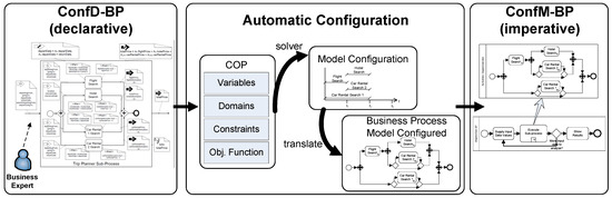
Figure 1.
Conf-BP Architecture.
4.1. Conf-BP Declarative Specification (ConfD-BP). A Formalization of the Language
The first stage of the framework is the specification of the configurable model in a declarative way. The declarative language and the grammar used in this step is DOOPT-DEC [15]. With the aim of better understand the type of problems solved in this article, the parts of the configurable declarative model are detailed in this section. The elements are shown in Figure 2, and they are described following. As the configurable system can be combined with other elements in a more complex work-flow, we provide the way to include the configurable description into a sub-process.
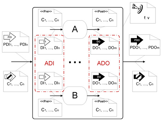
Figure 2.
Parts of the Configurable Declarative Description [15].
To introduce the formalization of the data provided and combined (see Figure 2), the different descriptions to include are divided into: (i) Sub-process description, including the descriptions of the components associated with the activities of the imperative part, detailed in Section 4.1.1; and (ii) Sub-process relationships, which is the declarative description of the relationships between the components through the data-flow (), addressed in Section 4.1.2.
4.1.1. Sub-Process Description
The sub-process description includes the components associated with the activities, gateways, and control-flow which are known and can be represented in an imperative way. Taking as the finite set of activities {, …, , …, } contained in a determined BP, the following definitions are introduced.
Definition 1.
and represent the sets containing, respectively, all the input data and output data involved in the execution of all the activities.
Within the set , containing all the input (output) variables, it is possible to identify the input (output) variables of each activity, defined as follows.
Definition 2.
and describe the set of input and output data of an activity involved in the sub-process, respectively, so that
Since various activities can share the same data input (or output), then it is also possible that:
The union of all the sets and all the sets of all the activities, constitute the sets and respectively, with non-repetitive elements.
Likewise, the specific variables that are inputs or outputs of the overall sub-process can be distinguished. They represent the information that flows from the customer to the sub-process and vice versa:
Definition 3.
is the set of input variables of the sub-process, which determines the information provided and defined by the customer. is composed of a subset of variables of .
Definition 4.
is the set of output variables of the sub-process. is composed of a subset of variables of .
4.1.2. Sub-Process Relationships
There exist different relationships between the data inputs and data outputs defined in the sub-process description. Those relationships are expressed as constraints, both at activity and at process level, giving rise to the sub-process relationships, with the following definitions:
Definition 5.
is the set of constraints that limits the specific values of the that must be satisfied to execute activity . Likewise, is the set of constraints that limits the specific values of the that must be satisfied after the execution of activity .
Definition 6.
() relates the values of variables of with variables of can take according to the values in each instance, and the possible values between the input and output of the activities.
Definition 7.
is an optimization function defined in terms of the data output of the activities ().
The objective of this optimization function is either to maximize or to minimize some of the output data that represents the business product, which constitutes the outcome of the process.
The result of this optimization problem is a set of input values that satisfies the objective function, the pre and post-conditions of the activities, and also satisfies the input and output constraints.
The set of input values that optimizes the output is found at runtime. The role of the constraints is to determine the possible values that this input and output data can take. All the constraints (, , , and ) are always defined at design time by a business expert who is familiar with the problem, although they are solved for each instance at runtime. Among every possible tuples of solutions that satisfy the constraints, the outcome of the sub-process will be the one which optimizes the variable defined in the optimization function.
4.1.3. Grammar
The elements used in the declarative description, describe the data relationship by means of numerical constraints. These constraints are defined by the following grammar, which is an extension of the grammar included in [15], where Variable and Constant, which represent the constant value for the variables, can be defined using Integer, Natural, Float, or String domains. On the other hand, Set can be defined as a set of Constant values of a specific Variable. The IF-THEN constraints have been included to DOOPT-DEC grammar [15], which are equivalent to the implication logic operator (→). IF-THEN constraints are used to represent that the relation of values between some data is conditioned to the value of others. The grammar of constraints is the following:
Constraint := ’IF’ General_Constraint’THEN’ General_Constraint| General_ConstraintGeneral_Constraint :_ Atomic_Constraint BOOL_OP General_Constraint| Atomic_Constraint| ‘¬’ Constraint| Variable SET_FUNCTION SetBOOL_OP:= ‘∨’ | ‘∧’SET_FUNCTION:= ‘∈’ | ‘∉’Atomic_Constraint:= function PREDICATE functionfunction:= Variable FUNCTION_SYMBOL function| Variable| ConstantPREDICATE:= ‘=’ | ‘≠’ | ‘<’ | ‘≤’ | ‘>’ | ‘≥’{For the String domain only ‘=’ and ‘≠’ are allowed }FUNCTION_SYMBOL:= ‘+’ | ‘−’ | ‘*’ | ‘/’{These operators are only applicable to Numerical variables}
4.1.4. Specification Applied to the Trip Planner Example
In the trip planner example, the activities involved in the model share some data, being necessary to create a work-flow aware data input and output. Figure 3 shows the trip example following the formalization detailed in the previous section and the notation described in [15].
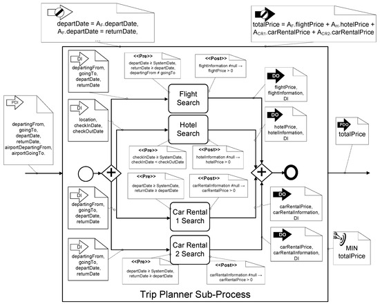
Figure 3.
Example of Trip Planner Formalization using DOOPT-DEC [15].
Hence, there are eight whose values are given by the customer:
- departingFrom: city from where the customer departs.
- goingTo: destination city.
- departDate: the day that the customer prefers to depart.
- returnDate: the day that the customer prefers to return.
- airportDepartingFrom: the departure airport to catch the flight.
- airportGoingTo: the arrival airport for the flight.
Four different activities are combined in order to perform the package trip offered to customers. This package trip is composed of flights, hotel rooms and, if necessary, the renting of a car to drive to an alternative departure airport, or from the arrival airport to the destination city. Each activity calculates the price as output of the activities for each data input. For the example, the activities () and their are:
- Flight Search Activity () returns the price of flights for a tuple of values for the data input.= {departingFrom, goingTo, departDate, returnDate}= {flightPrice, flightInformation, } where flightInformation = {outwardArrivalDate, returnArrivalDate, seat, number, …}The pre- and post-conditions of the activity A are:==
- Hotel Search Activity () is employed to ascertain the cost of booking a hotel room.= {location, checkInDate, checkOutDate}= {hotelPrice, hotelInformation, }The pre- and post-conditions of the activity A are:==
- Car Rental Search Activities ( and ) are employed to determine the price of renting a car. Two cars can be rented during the trip, one at the source () and another at the destination (). Nevertheless, the price of renting both cars is represented by , where , depends on these entries:= {departingFrom, goingTo, departDate, returnDate}= {carRentalPrice, carRentalInformation, }The pre- and post-conditions of the activity A are:==
Therefore, the output of the process, , are the outputs of the activities, which contain the information about the various components of the trip, as well as the total price of the trip ().
The customer only provides data to the sub-process: the eight . Then, each search activity only uses the necessary data, as detailed in its specification, for the searching. On the one hand, the sub-process can have input data that is not used by some search activity: for example, the Flight Search Activity takes the possible dates and cities given by the customer to the sub-process, meanwhile, the Hotel Search Activity takes the possible dates, the destination city and the preferences. The constraints between the input data of the sub-process and the activities are specified as the set of at design time. In the same way, the sub-process returns different data with respect to those returned by the activities, and it is necessary to define, at design time, how these data are calculated and related with the output data of the activities. Therefore, the set of define these relationships between the output data of the activities and the data returned by the sub-process to the customer. Although in the experimental evaluation all the constraints have been included, only the most representative constraints have been formulated in this section. Regarding the relationships between the data input and output that belong to the sub-process and the activities, the most representatives and are detailed below:
There are several numerical constraints that relate data input and output belonging to the process and the activities. Some of the constraints are defined below:
- :
- -
- The constraints that establish the values of departure date () and return date () of the flights have to coincide with the input data proposed by the customer.
- -
- The constraints that describe the values of the departure airport () and arrival airport () of the flight have to coincide with the input data proposed by the customer.
- -
- The date of check-in into the hotel should coincide with the arrival date of the outward flight ().
- -
- If the flight does not depart from the departure location (), then the rental of a car () is necessary.
- -
- If the flight arrives at the destination city , then it is not necessary to rent a car at the destination city.
- -
- If the flight does not depart from the departure location (), then the rental of a car () is necessary.
- :
- -
- The total price is the sum of all the prices returned by the activities, as presented in constraint ().
In this example, the optimization involves the minimization of the total price of the trip, which is composed of the cost of buying flight tickets, staying in a hotel room, and renting cars for the departure and arrival cities.
4.2. Conf-BP Imperative Modelling (ConfM-BP)
Once the declarative model is described, it can be possible to obtain an imperative model that satisfies the data dependencies. Between the different options, we propose the most optimal, according to the execution time of the instances of the process. To model the BP work-flow in an imperative way, the standard BPMN [47] is chosen, since it is supported by several commercial BPMS. The activities will be combined in a sub-process that starts and ends with the corresponding events. The various order combination of the activities will be represented with a sequence or by means of the control flows: parallel, exclusive or inclusive execution.
Figure 4 shows how the imperative configuration obtained from the declarative description is included in a business process model. The activity “Supply Input Data Values” provides the input data values used during the process execution. As was commented before, sometimes the most appropriate input data to optimize the business product are unknown at design time, since it depends on each instance. The used example, the trip planner, has these characteristics, since the dates and city airport must be found, as detailed in [15]. The sub-process “Execute sub-process” represents the imperative model that should be created according to the data dependencies described and detailed in the following sections. This sub-process is formed of the set of activities involved in the declarative model by means of the BPMN connections and gateways as detailed in Section 4.3. Several possible imperative models exist that satisfy the data dependencies, but our objective is to find the optimal model with respect to execution time of any instantiation of the BP.
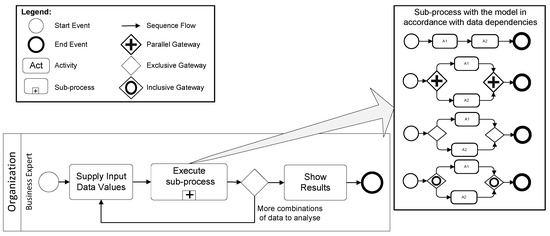
Figure 4.
Imperative Representation of the Declarative Model.
A simplification of the possibilities of the problem are shown in Figure 5, where only the activities “Flight Search” and “Car Rental 1 Search” are considered for the modelling configuration. Analyzing the five possibilities we can find out that: (a) and (b) describe a sequence relation between two activities that can mean that one of the activities has priority order over the another activity, for the example it will be used if ‘Car Rental 1’ cannot be executed until ‘Flight Search’ ends or vice versa, and; (c), (d) and (e) represent the execution of one (XOR gateway), more than one (or gateway), or every activities at the same time. For the example it will be used if there not exists an order dependency between the activities. Therefore, which is the best model option to satisfy our trip problem?
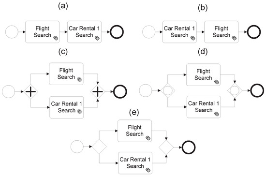
Figure 5.
“Flight Search” and “Car Rental 1 Search” Model Possibilities.
This modelling combination and analysis increase considerably as soon as the number of activities grows. Hitherto, this configuration has been made by human experts, we propose obtain it automatically in the Conf-BP Framework. Therefore, in order to transform this declarative model into an imperative model that supports any value of input variables of the process by considering the data dependencies, we propose the use of the Constraint Programming paradigm, as explained in Section 4.3.
4.3. Automatic Transformation from Declarative to Imperative Model
The transformation from the declarative description into an imperative model is a difficult and hard task, since it implies the analysis of every possible configuration to obtain at design time the most optimal model at runtime. The difficulty lies in establishing the order of the activities and the control flow components that combine the activities, taking into account the data dependencies. To perform the optimal transformation, we propose the three steps shown in Figure 6.
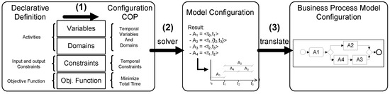
Figure 6.
Configuration problem Transformation.
- Create a Constraint Optimization Problem using the declarative Model: As explained in detail in Section 4.3.1, we used Constraint Satisfaction Problems (CSPs) [48] to solve the configuration problem.CSPs represent a reasoning methodology consisting of the representation of a problem by means of a set of variables, domains and constraints. CSPs have also a declarative description, then very similar to the Declarative Specification of ConfD-BP. CSPs are a widely used model-based knowledge representation formalism. In a formal way, it is defined as a tuple ⟨X, D, C⟩, where {, , …, } is a finite set of variables, {, , …, } is a set of domains of the values of the variables, and {, , …, } is a set of constraints. A constraint specifies the possible values of the variables in that simultaneously satisfy . Let {, , …, } be a subset of X, and an l-tuple (, , …, ) from , , …, can therefore be called an instantiation of the variables in . An instantiation is a solution if and only if it satisfies the constraints C. If an objective function is included in the CSP, it is called a Constraint Optimization Problem (COP). It is necessary to highlight that CSP and COP specifications are very similar to the process models proposed here, since both are declarative models which define the problem but do not solve it. A solver of CSPs or COPs tries to find a possible tuple of values for the variables that satisfy the constraints defined in the domain.
- Solve the COP: To solve the COP created in the second step, it is necessary to analyze the possible values of the variables to find the satisfied tuples. To avoid the analysis of every possibilities of values of variables, the solvers use a combination of search and consistency techniques [49] reducing drastically the complexity and time consuming. The consistency techniques remove inconsistent values from the domains of the variables during or before the search. Several local consistency and optimization techniques have been proposed as ways of improving the efficiency of search algorithms. There are several commercial constraint problem solvers. The main difference between them is the programming language that they use, and the types of constraints that can be included. For the proof of concept to validate the configuration problem, we have used JsolverTM [50], although any of the existing CSP solvers could be used, since the constraints that we need to include (explained in Section 4.3.1) are very common and supported by every commercial solvers. The resolution of the COP will obtain a set of time intervals, each of them associated with an activity, representing the moment when each activity can start and end.
- Translate the COP solution into a BPMN Model: As explained in detail in Section 4.3.2, by using the results obtained from the COP, the imperative model can be created. This result has to be interpreted as gateways that relate the activities. For example, if the COP allows that two activities A and B could start at the same instant of time, perhaps there is a constraint which states that only one activity can be executed in each instance. In that case, there can be an exclusive or inclusive gateway relating the two activities. The decision between the possible gateways between the various activities is based on: (a) the study of the domains of the data related in the declarative problem description, and; (b) the data obtained from the resolution of the COP as it is explained in Section 4.3.2.
4.3.1. Configuration of a BP Model: Creating a COP from the Declarative Model
The relation between the input and output of the activities determines their relational order. For the same declarative model, it is possible to find several configurations of activities that satisfy the requirements and description. To find the best configuration, we propose the use of an intelligent system to find the optimal BP model that maximizes the parallelism of the activities, with the aim of minimizing the execution time. To determine this configuration, we suggest the transformation of the declarative model into a COP, to analyze the possible instant when the activities can start and end their executions, according to data dependency.
Firstly, and before to explain how to create the COP, it is necessary as a previous step to ascertain the data relation, especially when they are included in the IF-THEN constraints of the description of the problem. The definition of Tuple of Condition-Relation in order to introduce this relation is introduced.
Definition 8.
A Tuple of Condition-Relation is a tuple formed of , where represents under which condition is executed after . Therefore, the value in the implies that is always executed after , or, in the case when the contains an expression, is executed after if and only if the expression is met.
These tuples are built analyzing the data relations found in the set of and that describe the declarative model. For each constraint where the output of an activity is related to the input of an activity , a tuple is created. If the input-output relation appears in an IF-THEN constraint with a c condition, the tuple will be ⟨c, , ⟩, and ⟨, , ⟩ otherwise.
With the list of intervals and the list of tuples of data relations, the following COP is created:
- Variables: The possible instants when each activity can be executed, are defined as the tuple of variables , where is the instant of time in which the activity begins, and is the instant of time in which the activity finishes. For each activity , the COP will include a couple of variables . To represent the execution time of the whole process, the variable T is included, that represents the of the last activity executed. If every activities is executed in parallel, T will be the maximum value of , but if every activities are executed sequentially, the value of T will be the summation of every .
- Domain: The domain of the and variables is related to the execution time of each activity. If we suppose that each activity spends units of time, then the domain of each variable is:
- -
- : 0..
- -
- : ..
- -
- T: max()..
- Constraints: The necessary constraint to model the COP are:
- -
- It is mandatory that for every activity , ≤
- -
- T has to be the greatest value of t, then T ≥ for every A.
- -
- For each element of the list of tuples building by using the data relations, a numerical constraint is included in the COP. Each relation between data input and output in the way ⟨c, , ⟩ is translated into the constraint ≥ . For example, in the trip planner, the constraint is translated into . Therefore, all the activities could start at the same instant unless there exists a relationship requiring one activity to start after another.
- Objective: The optimization function of the COP is the minimization of the total time, it implies to minimize the value of T (minimization(T)).
Table 1 gives a summary of the equivalence of the elements of the formalization and the COP built.

Table 1.
Declarative model and COP elements relationship.
The solving of the COP will obtain a pair of start and end instants of time for each activity that minimizes any instantiation time (T) for the model. As mentioned earlier, the minimum execution time of an activity is modelled as a units of time. But it is possible to obtain the same value of (T), where the execution time is minimized, with different and for the same problem. Suppose activities (, , and ) that last a unit of time, where the input data of depends on the output of , and the input data of depends on the output of . Figure 7 depicts two possible configurations (a) and (b) that minimize the theoretical execution time (). However, there exist more variations, since can be executed in a parallel way with any of the other activities.
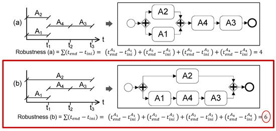
Figure 7.
Flexibility of the BP in terms of the execution time of the Activities.
Although both options (a) or (b) are optimal according time consuming, the model of Figure 7b is better than the model of Figure 7a, since it supports an unexpected delay of executing, not increasing the total execution time ().
To make the imperative model more robust to unexpected delays, we propose to modify the proposed COP to find the most paralleled process. To this end, the COP must find the greatest value of for each . It is obtained including the variables as a goal in the COP, and leaving the domain of open during the search. Then, the variables will be instantiated during the propagation phase, while all the possible values of the domains of variables will be obtained as solutions of the COP for each value of . The greatest value of the domain is the most appropriate value to build an imperative robust business process model.
Algorithm 1 describes the creation of the COP from a declarative specification as explained before.
| Algorithm 1 Creation of a COP from a Declarative Specification. |
|
4.3.2. Transformation of the COP results into a BP Imperative Model
The list of time intervals, obtained from the COP, with the most appropriate values for and for each activity, has to be translated into an imperative BP model. For the example of Figure 7b, the obtained list is: {, , , }. There exist various imperative models in business processes, but the most widely used standard language is BPMN [47]. Although the model in the standard is represented by means of an XML file, to facilitate the understanding of the algorithm that obtains the imperative model, we propose the use of a BPMN-Graph. As explained in [1], BPMN is a graph-oriented language in which control and action nodes can be connected. Therefore, we propose to model the BPMN using a directed graph as defined in [51].
The problem is solved in two steps: firstly, the BPMN-Graph is built not specifying the type of gateways, only including which are splits and joins, and; secondly, the uncertain about the gateways is solved analyzing the list of tuples created in function of the IF-THEN constraints of the model, that related the activity execution on function of the value of other variables.
Step 1: Building BPMN-Graph
The proposed BPMN-Graph is a direct graph composed of: (i) vertices, which represent the activities and the gateways; and (ii) edges, which represent the sequence flows that join the various vertices. Firstly, the idea of the algorithm is explained by means of a trace, after which the algorithm is detailed. Analyzing the and of each activity, it is possible to discover the activities that have parallel or sequential relation between them. The main idea of the algorithm is to detect these relations by building sub-graphs, that will be combined in a sequential or parallel way. An example of the trace of the algorithm is shown in Figure 8. The initial is formed by a set of activities , associated with a time interval , and a list of tuples that describe the condition about the activities order dependencies. The algorithm divides the problem in function of the sequential points and the parallel subsets. Both definitions are introduced:
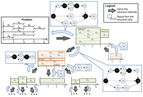
Figure 8.
Trace example of the Algorithm to create a BPMN-Graph using the COP results.
Definition 9.
Sequential point (List of Time Intervals): For a List of Time Intervals, a sequential point is an instant, or set of instants of time at which no activity can be executed. It implies that in a sequential point, only the execution of an activity can start or end, and therefore the problem can be broken into two smaller that can be executed sequentially.
Definition 10.
Parallel subsets (List of Time Intervals, List of Tuples of Relations):For a list of Time Intervals associated with the activities … , the parallel subsets are a set of subset of activities , …, , where there does not exist any activity a ∈ and an activity b ∈ , where ≠ , such that there exists a tuple in the List of Tuples of Relations that ⟨condition, a, b⟩. A way to obtain the parallel subsets, is creating a parallel subset for each activity (, …, ), if there exist an activity a ∈ and another activity b ∈ , both subsets are merged. This process is repeated until no more sets can be merged.
With the aim of facilitating the understanding of the algorithm and our proposal in general, we use the example of Figure 8, with the list of tuples:
- (R1) , ,
- (R2) , ,
- (R3) , ,
- (R4) , ,
- (R5) ,
- (R6) , ,
- (R7) ,
The trace follows the next steps:
- Look for sequential points: Firstly, the set of activities should be separated by the sequential points (arrow 1 in Figure 8). The separation is carried out by detecting those instants of time where there is a sequential point. The intervals that are derived from these sequential points delimit the subset of activities. In the example, the set of activities is separated into two subsets of activities, since there is only one sequential point in . The first subset goes from to and includes all activities except activity . On the other hand, the second subset goes from to and only includes activity .
- Solving sequential sub-problems: Each subset of activities is solved as a sub-problem (arrows 2 and 3) and combined sequentially both BPMN-sub-graphs are solved.
- Look for parallel subsets: The is separated in three parallel subsets: , and . To obtain these subsets, the idea described in Definition 10 is applied:
- (a)
- Create a subset of each activity: {: {}, : {}, : {}, : {}, : {}, : {}, : {}}.
- (b)
- Since is related with in , and with in , both subsets are merged. Also, and are related in . The obtained parallel subsets are: {: {, , }, : {}, : {}, : {, }}.
- (c)
- Since is related with in , and with in , both subsets are merged. Therefore, the parallel subsets: {: {, , , }, : {}, : {, }} are also obtained.
- (d)
- Tuple relations and are not used in the creation of subsets since is not involved in the parallel analysis.
- Solving parallel sub-problems: The next step implies to solve each sub-problem (arrows 4, 5 and 6), followed by the search of sequential points.
- Combining parallel sub-problems: To solve it is necessary to combine the sub-graphs obtained by solving , and (return of arrow 4, 5 and 6). These BPMN-sub-graphs are combined as various branches joined by a split and join node ( in the example).
- Combining sequential sub-problems: The obtained results after a sequential analysis of sub-graphs (returns of arrow 2 and 3) implies joining the results of and . To this end, the result (BPMN-Graph) of and are joined by an edge between the final vertex of and the initial vertex of , which are and respectively.
| Algorithm 2 Create a BP model from COP result. |
|
Algorithm 2 details the procedures for the sequential and parallel treatments explained above. Algorithm 2 takes a and transforms it into a BPMN-Graph. Initially, the is treated sequentially with the algorithm , which finds the sequential points following Definition 9. Each of the found, has to be analyzed to identify the parallel subsets of activities with the algorithm (following Definition 10). The parallel treatment of a consists of gathering the activities that are related into subsets and creating new problems from these subsets. The relationships among the activities are given by the tuples of Condition-Relation of the . Each is then solved recursively. To combine the parallel subsets, two gateway vertices are inserted as split and join gateway respectively. Each BPMN-sub-graph will be a branch related by means of the gateway. To combine two sequential BPMN-sub-graphs, only and edge needs to be included between the last node of the first solution and the first node of the second solution. The algorithm draws to a halt when reaching a base case, or when the problem contains only one activity. In both treatments, the solution of a base case is a graph with a unique vertex that represents this activity.
Step 2: Defining The Gateways
Once the graph is created, the correct gateways that diverge the sequence flows have to be selected. In the graph, the gateways are identified by means of studying the tuples of Condition-Relation obtained from the constraints, defined in the declarative specification.
The different types of relations described by means of the tuples of Condition-Relation, and how they affect to the type of gateway are explained below:
- Parallel: two activities are executed in a parallel way if there are no conditions that relate the of both activities (see Figure 9).
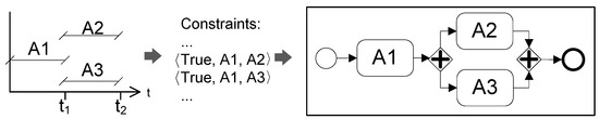 Figure 9. Parallel Relationship.
 - Exclusive: two activities are executed in an exclusive way if the constraints that relate the of the two activities and the domain of these constraints are complete and do not overlap. For example, as shown in Figure 10, if the execution of and depends on a value of the output data , but there are no overlaps ( is executed when is less than 50 and is executed when is greater than or equal to 50), then there is an exclusive relationship between them. There is another possibility when only one condition is described, for example only exists the condition ( is executed when is less than 50), in that case it means that there are two branches for the XOR gateway, but one of them with no activities.
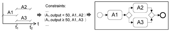 Figure 10. Exclusive Relationship.
 - Inclusive: two activities are executed in an inclusive way if there are conditions that relate the of both activities, and the domain of these conditions are complete and overlapped. For example, as shown in Figure 11, if the execution of and depends on a value of the output data , but there are overlaps between the domains that satisfy the constraints ( is executed when is less than 75 and is executed when is greater or equal to 25, and hence both coincide when is greater than 25 and less than 75), then there is an inclusive relationship.
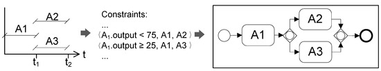 Figure 11. Inclusive Relationship.
Table 2 gives a summary of the resulting gateways depending on the conditions established by the constraints that relate the data of the activities.
Table 2.
Type of gateway decision.
For the example explained in Figure 8, it is necessary to analyze and (see Figure 12). Since there are no relations between activities , , and , then is a parallel gateway. On the other hand, the execution of activities and depends on the outputs of . The conditions specified in relations and indicate that the domain of the constraints is complete and there are no overlaps, therefore, is an exclusive gateway.
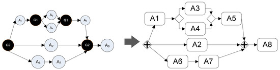
Figure 12.
From graph to BPMN Model Example.
5. Results: Transformation Applied to the Trip Planner Example
To illustrate the use of the algorithms, the application of the algorithms to the Trip Planner example is presented in this section.
The first step is to obtain the list of tuples of Condition-Relation according Definition 8. Analyzing the constraints of the example, we can find: (i) Constraints C1, C2, C3, and C4 do not relate input and output of the activities, then they are not involved in the list of tuples of Condition-Relation; (ii) Constraint C5 is used to create the relation: ⟨, , ⟩; (iii) Constraint C6 is used to create the tuple: ⟨Condition of , Start_Event, ⟩; (iv) Constraint C7 creates the same tuple than Constraint C5: ⟨, , ⟩, and; (v) Constraint C8 is used to create the tuple: ⟨Condition of , , ⟩}.
After that, the second step is to build the COP as detailed in Section 4.3.1, that for the example will have the form.
- Variables:, , , , , , , , T.
- Domain: Supposing that the theoretical execution time of each activity is a unit of time, the domains are:
- -
- , , , : 0..3 //Since there are 4 different activities.
- -
- , , , : 1..4
- -
- T: 1..4
- Constraints:
- -
- ≤
- -
- ≤
- -
- ≤
- -
- ≤
- -
- T ≥ ∧ T ≥ ∧ T ≥ ∧ T ≥
- -
- For the list of tuples of Condition-Relation mentioned above, the constraints included in the COP are:
- ∗
- ≥
- ∗
- ≥
- Goal:, , ,
- Objective: minimization(T).
The obtained values of the variables after the resolution of the COP are:
- : 2
- : 0 and : 1
- : 1 and : 2
- : 0 and : [1..2], selecting the greatest value (2).
- : 1 and : 2
The resulting BP Model is shown in Figure 13. According to the results, “Flight Search” and “Car Rental 1 Search” activities start at instant 0. However, the “Car Rental 2 Search” activity depends on the value of the output data of the “Flight Search” activity, so there is an exclusive gateway before this activity. Since there is not a complete domain with the constraint that determines the execution of the “Car Rental 2 Search” activity, then there is a branch by default which indicates that nothing happens when the condition is not met. The same situation occurs with “Hotel Search” and “Car Rental 2 Search” activities.
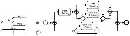
Figure 13.
Trip Planner Model Result.
The solution parallelizes the activities according to the data input and output relations, being possible execute it in two units of times.
Empirical Evaluation
Since the generated imperative only depends on the declarative model, it is created only once at design time. The transformation performed involves a COP and two own-developed algorithms. Therefore, the critical points of our proposal lies in the resolution of the COP and these algorithms.
Regarding the resolution of a COP, we use one of the existing commercial tools to evaluate the COP, since the COP resolution has remained a known problem studied by researchers in the area over several decades, and is supported by an important set of tools used in real problems. In general, the time to find the solution of a COP depends on: (1) the type of constraints (lineal, polynomial); (2) the number of constraints; and (3) the number and type of the variables. It is possible to find an analysis in [52] on the complexity of the NP-complete constraint problem resolution according to these characteristics. The complexity of resolution of CSPs depends on the number of possible solutions of the problem, and on whether it is neither under constraint nor unsolvable. The most complex of these problems are those that are neither under constraint nor unsolvable. For these reasons, no affirmation can be given concerning the efficiency in a generic way of our proposal, since our declarative specification enables any type and any number of constraints; therefore the evaluation time depends on the specific problem. Depending on the number of constraints associated with a COP, and the number of variables, the COP evaluation time remains variable.
On the one hand, in relation to Algorithms 1 and 2, the computational order is linear since it only depends on the number of activities. On the other hand, Algorithm 2 defines two recursive functions which are related between each other. The main idea of this algorithm is to apply a Divide-and-Conquer Method by means of reducing the problem in sub-problems, being the smallest problem, in our case, a single activity. Therefore, in both the best and the worst cases, the computational order is linear since it depends on the number of activities either they have a parallel or sequential relationships.
With the aim of performing the evaluation, both algorithms are executed over a set of 50 generated test cases (see Table 3). Each test case establishes a different number of activities with a set of and constraints that relate them. On the one hand, as explained before, the number of activities determines the complexity of solving the problem. On the other hand, the number of and the constraints determine the structure of the final imperative business process.
Table 3.
Summary of the test cases used for evaluation.
Figure 14 shows the computing time needed to solve both algorithms. The test cases are measured using a PC with an Intel Core i7-2675QM CPU with a 2.2 GHz processor and a 8 GB of RAM.
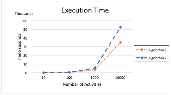
Figure 14.
Execution Time of Algorithm 1 and Algorithm 2.
6. Conclusions and Future Work
Declarative languages have been focused on the order of activities, and not on how the data values and dependencies can affect the optimal execution of a process. In this paper, we apply configuration problems ideas to the construction of an imperative model according to the declarative description of the data relation. Our proposal shields the business experts from unnecessary details, and to provide assistance when experts know what they want (the BP requirements by means of data dependencies) but do not know how to attain what they want (establish the order of the activities), Conf-BP Framework is proposed. Conf-BP establishes a methodology to transform a declarative model into an imperative representation using BPMN. Business experts only have to specify the BP requirements, leaving the configuration of the activities in the imperative model to the intelligent system, which uses the Constraint Programming paradigm and a set of proposed definitions and algorithms. This automatic methodology obtains an imperative model described by BPMN where the optimal model related to execution time is obtained. In addition, the framework is applied to an example: the process of organising a trip. Future work into this area involves increasing the capabilities of Conf-BP by including loops within the model, where there exists a cyclic relation between the data.
Author Contributions
Conceptualization and Methodology, L.P. and M.T.G.-L.; Development, L.P.; Validation, M.T.G.-L. and A.J.V.-V.; Writing-Original Draft, L.P.; Writing—Review & Editing, M.T.G.-L., A.J.V.-V., and R.M.G.
Funding
This work has been partially funded by the Ministry of Science and Technology of Spain (TIN2015-63502-C3-2-R) and the European Regional Development Fund (ERDF/FEDER).
Conflicts of Interest
The authors declare no conflict of interest.
Abbreviations
The following abbreviations are used in this manuscript:
| ADI | Activities Data Input |
| ADO | Activities Data Output |
| BP | Business Process |
| BPEL | Business Process Executation Language |
| BPM | Business Process Management |
| BPMN | Business Process Model and Notation |
| BPMS | Business Process Management System |
| Conf-BP | Configuration of Activities in Business Processes |
| ConfD-BP | Conf-BP Declarative Specification |
| ConfM-BP | Conf-BP Imperative Modelling Specification |
| COP | Constraint Optimization Problem |
| CSP | Constraint Satisfaction Problem |
| OBJ_FUNC | Objective Function |
| PDI | Process Data Input |
| PDO | Process Data Output |
References
- Weske, M. Business Process Management: Concepts, Languages, Architectures; Springer: Berlin, Germany, 2007. [Google Scholar]
- Aguilar-Saven, R.S. Business process modelling: Review and framework. Int. J. Prod. Econ. 2004, 90, 129–149. [Google Scholar] [CrossRef]
- Tsai, A.; Wang, J.; Tepfenhart, W.; Rosea, D. EPC Workflow Model to WIFA Model Conversion. In Proceedings of the IEEE International Conference on Systems, Man and Cybernetics, SMC ’06, Taipei, Taiwan, 8–11 October 2006; Volume 4766/2007, pp. 2758–2763. [Google Scholar]
- Sinogas, P.; Vasconcelos, A.; Caetano, A.; Neves, J.; Mendes, R.; Tribolet, J.M. Business Processes Extensions to UML Profile for Business Modeling. ICEIS 2001, 2, 673–678. [Google Scholar]
- List, B.; Korherr, B. A UML 2 Profile for Business Process Modelling. In Proceedings of the ER (Workshops), Klagenfurt, Austria, 24–28 October 2005; pp. 85–96. [Google Scholar]
- Bosilj-Vuksic, V.; Hlupic, V. Petri Nets and IDEF diagrams: Applicability and efficacy for business process modelling. Int. J. Comput. Inform. 2001, 25, 123–133. [Google Scholar]
- Pichler, P.; Weber, B.; Zugal, S.; Pinggera, J.; Mendling, J.; Reijers, H.A. Imperative versus Declarative Process Modeling Languages: An Empirical Investigation. In Business Process Management Workshops; Lecture Notes in Business Information Processing; Springer: Berlin, Germany, 2011; Volume 99, pp. 383–394. [Google Scholar]
- Zugal, S.; Soffer, P.; Haisjackl, C.; Pinggera, J.; Reichert, M.; Weber, B. Investigating expressiveness and understandability of hierarchy in declarative business process models. Softw. Syst. Model. 2015, 14, 1081–1103. [Google Scholar] [CrossRef]
- Fahland, D.; Lubke, D.; Mendling, J.; Reijers, H.; Weber, B.; Weidlich, M.; Zugal, S. Declarative versus Imperative Process Modeling Languages: The Issue of Understandability. In Enterprise, Business-Process and Information Systems Modeling; Lecture Notes in Business Information Processing; Springer: Berlin/Heidelberg, Germany, 2009; Volume 29, pp. 353–366. [Google Scholar]
- Fahland, D.; Mendling, J.; Reijers, H.; Weber, B.; Weidlich, M.; Zugal, S. Declarative versus Imperative Process Modeling Languages: The Issue of Maintainability. In Business Process Management Workshops; Lecture Notes in Business Information Processing; Springer: Berlin/Heidelberg, Germany, 2010; Volume 43, pp. 477–488. [Google Scholar]
- Sadiq, S.W.; Orlowska, M.E.; Sadiq, W. Specification and validation of process constraints for flexible workflows. Inf. Syst. 2005, 30, 349–378. [Google Scholar] [CrossRef]
- Rychkova, I.; Regev, G.; Wegmann, A. High-level design and analysis of business processes: The advantages of declarative specifications. In Proceedings of the Second International Conference on Research Challenges in Information Science, RCIS 2008, Marrakech, Morocco, 3–6 June 2008; Pastor, O., Flory, A., Cavarero, J.L., Eds.; pp. 99–110. [Google Scholar]
- Pesic, M.; van der Aalst, W.M.P. A Declarative Approach for Flexible Business Processes Management. In Business Process Management Workshops; Lecture Notes in Computer Science; Eder, J., Dustdar, S., Eds.; Springer: Berlin, Germany, 2006; Volume 4103, pp. 169–180. [Google Scholar]
- Rychkova, I.; Regev, G.; Wegmann, A. Using Declarative Specifications in Business Process Design. IJCSA 2008, 5, 45–68. [Google Scholar]
- Parody, L.; Gómez-López, M.T.; Gasca, R.M. Hybrid business process modeling for the optimization of outcome data. Inf. Softw. Technol. 2016, 70, 140–154. [Google Scholar] [CrossRef]
- Van der Aalst, W.M.P. Process Mining: Data Science in Action, 1st ed.; Springer: Berlin/Heidelberg, Germany, 2016. [Google Scholar]
- Fernández-Cerero, D.; Fernández-Montes, A.; Jakóbik, A.; Kołodziej, J.; Toro, M. SCORE: Simulator for cloud optimization of resources and energy consumption. Simul. Model. Pract. Theory 2018, 82, 160–173. [Google Scholar] [CrossRef]
- Teppan, E.C.; Friedrich, G. The Partner Units Configuration Problem. arXiv, 2013; arXiv:1308.6206. [Google Scholar]
- GröNer, G.; BošKović, M.; Silva Parreiras, F.; GašEvić, D. Modeling and Validation of Business Process Families. Inf. Syst. 2013, 38, 709–726. [Google Scholar] [CrossRef]
- Petrie, C.J. Automated Configuration Problem Solving; Springer Publishing Company: New York, NY, USA, 2012. [Google Scholar]
- Gillmann, M.; Mindermann, R.; Weikum, G. Benchmarking and Configuration of Workflow Management Systems. In Cooperative Information Systems; Springer: Berlin/Heidelberg, Germany, 2000; Volume 1901, pp. 186–197. [Google Scholar]
- Van der Aalst, W.M.P.; van Hee, K. Workflow Management: Models, Methods, and Systems; MIT Press: Cambridge, MA, USA, 2004. [Google Scholar]
- Czarnecki, K.; Helsen, S.; Eisenecker, U. Formalizing cardinality-based feature models and their specialization. Softw. Process Improv. Pract. 2005, 10, 7–29. [Google Scholar] [CrossRef]
- Gottschalk, F.; van der Aalst, W.M.P.; Jansen-Vullers, M.H.; Rosa, M.L. Configurable Workflow Models. Int. J. Coop. Inf. Syst. 2008, 17, 177–221. [Google Scholar] [CrossRef]
- La Rosa, M.; van der Aalst, W.M.P.; Dumas, M.; ter Hofstede, A.H.M. Questionnaire-based variability modeling for system configuration. Softw. Syst. Model. 2009, 8, 251–274. [Google Scholar] [CrossRef]
- Moon, M.; Hong, M.; Yeom, K. Two-Level Variability Analysis for Business Process with Reusability and Extensibility. In Proceedings of the 2008 32nd Annual IEEE International Computer Software and Applications Conference, Turku, Finland, 28 July–1 August 2008; pp. 263–270. [Google Scholar]
- Reijers, H.; Mans, R.; van der Toorn, R. Improved model management with aggregated business process models. Data Knowl. Eng. 2009, 68, 221–243. [Google Scholar] [CrossRef]
- Kumar, A.; Yao, W. Design and management of flexible process variants using templates and rules. Managing Large Collections of Business Process Models. Comput. Ind. 2012, 63, 112–130. [Google Scholar] [CrossRef]
- Baran, M.; Kluza, K.; Nalepa, G.J.; Ligęza, A. A hierarchical approach for configuring business processes. In Proceedings of the 2013 Federated Conference on Computer Science and Information Systems, Krakow, Poland, 8–11 September 2013; pp. 915–921. [Google Scholar]
- Albert, P.; Henocque, L.; Kleiner, M. An End-to-End Configuration-Based Framework for Automatic SWS Composition. In Proceedings of the 20th IEEE International Conference on Tools with Artificial Intelligence, Dayton, OH, USA, 3–5 November 2008; Volume 1, pp. 351–358. [Google Scholar]
- Bertoli, P.; Pistore, M.; Traverso, P. Automated composition of Web services via planning in asynchronous domains. Artif. Intell. 2010, 174, 316–361. [Google Scholar] [CrossRef]
- Mesmoudi, A.; Mrissa, M.; Hacid, M.S. Combining configuration and query rewriting for Web service composition. In Proceedings of the IEEE International Conference on Web Services (ICWS), Washington, DC, USA, 4–9 July 2011; pp. 113–120. [Google Scholar]
- Drescher, C. The Partner Units Problem a Constraint Programming Case Study. In Proceedings of the IEEE 24th International Conference on Tools with Artificial Intelligence, ICTAI 2012, Athens, Greece, 7–9 November 2012; pp. 170–177. [Google Scholar]
- Mittal, S.; Frayman, F. Towards a Generic Model of Configuraton Tasks. In Proceedings of the 11th International Joint Conference on Artificial Intelligence, San Francisco, CA, USA, 20–26 August 1989; Volume 2, pp. 1395–1401. [Google Scholar]
- Rosa, M.L.; Dumas, M.; ter Hofstede, A.H.M.; Mendling, J. Configurable multi-perspective business process models. Inf. Syst. 2011, 36, 313–340. [Google Scholar] [CrossRef]
- Van der Aalst, W.M.P.; Dumas, M.; Gottschalk, F.; ter Hofstede, A.H.M.; Rosa, M.L.; Mendling, J. Correctness-Preserving Configuration of Business Process Models. In Proceedings of the 11th International Conference on Fundamental Approaches to Software Engineering, FASE 2008, Budapest, Hungary, 29 March–6 April 2008; Held as Part of the Joint European Conferences on Theory and Practice of Software, ETAPS 2008; Lecture Notes in Computer Science. Fiadeiro, J.L., Inverardi, P., Eds.; Springer: Berlin, Germany, 2008; Volume 4961, pp. 46–61. [Google Scholar]
- Rosemann, M.; van der Aalst, W.M.P. A configurable reference modelling language. Inf. Syst. 2007, 32, 1–23. [Google Scholar] [CrossRef]
- Vanderfeesten, I.; Reijers, H.A.; van der Aalst, W.M. Product-based workflow support. Inf. Syst. 2011, 36, 517–535. [Google Scholar] [CrossRef]
- Vanderfeesten, I.T.P.; Reijers, H.A.; van der Aalst, W.M.P. Product Based Workflow Support: Dynamic Workflow Execution. Lecture Notes in Computer Science. In Proceedings of the 20th International Conference on Advanced Information Systems Engineering, CAiSE 2008, Montpellier, France, 16–20 June 2008; Bellahsene, Z., Léonard, M., Eds.; Springer: Berlin, Germany, 2008; Volume 5074, pp. 571–574. [Google Scholar]
- Kluza, K.; Honkisz, K. From SBVR to BPMN and DMN Models. Proposal of Translation from Rules to Process and Decision Models. In Artificial Intelligence and Soft Computing; Rutkowski, L., Korytkowski, M., Scherer, R., Tadeusiewicz, R., Zadeh, L.A., Zurada, J.M., Eds.; Springer International Publishing: New York, NY, USA, 2016; pp. 453–462. [Google Scholar]
- Object Management Group (OMG). Semantics of Business Vocabulary and Business Rules (SBVR); Version 1.4: Formal Specification; OMG: Needham, MA, USA, 2017. [Google Scholar]
- Natschläger, C.; Kossak, F.; Schewe, K.D. Deontic BPMN: A powerful extension of BPMN with a trusted model transformation. Softw. Syst. Model. 2015, 14, 765–793. [Google Scholar] [CrossRef]
- Wiśniewski, P.; Kluza, K.; Ligęza, A. An Approach to Participatory Business Process Modeling: BPMN Model Generation Using Constraint Programming and Graph Composition. Appl. Sci. 2018, 8, 1428. [Google Scholar] [CrossRef]
- Borrego, D.; Eshuis, R.; López, M.T.G.; Gasca, R.M. Diagnosing correctness of semantic workflow models. Data Knowl. Eng. 2013, 87, 167–184. [Google Scholar] [CrossRef]
- Vanhatalo, J.; Völzer, H.; Leymann, F.; Moser, S. Automatic Workflow Graph Refactoring and Completion. In Proceedings of the Service-Oriented Computing–ICSOC 2008, Sydney, Australia, 1–5 December 2008; Bouguettaya, A., Krueger, I., Margaria, T., Eds.; Springer: Berlin/Heidelberg, Germany, 2008; pp. 100–115. [Google Scholar]
- Hasanov, E. Enhancing BPMN Conformance Checking with OR Gateways and Data Objects. Ph.D. Thesis, University of Tartu, Tartu, Estonia, 2017. [Google Scholar]
- Object Management Group (OMG). Business Process Model and Notation (BPMN) Version 2.0; Object Management Group Standard; OMG: Needham, MA, USA, 2011. [Google Scholar]
- Rossi, F.; van Beek, P.; Walsh, T. Handbook of Constraint Programming (Foundations of Artificial Intelligence); Elsevier Science Inc.: New York, NY, USA, 2006. [Google Scholar]
- Dechter, R. Constraint Processing; Elsevier Morgan Kaufmann: Burlington, MA, USA, 2003; Available online: https://www.ibm.com/es-es/marketplace/ibm-ilog-cplex (accessed on 20 October 2018).
- Manual, R. JSolver 2.1. Available online: https://www.ibm.com/es-es/marketplace/ibm-ilog-cplex (accessed on 24 February 2014).
- Gómez López, M.T.; Gasca, R.M.; Pérez-Álvarez, J.M. Decision-Making Support for the Correctness of Input Data at Runtime in Business Processes. Int. J. Coop. Inf. Syst. 2014, 23, 1450003. [Google Scholar] [CrossRef]
- Cheeseman, P.; Kanefsky, B.; Taylor, W.M. Where the Really Hard Problems Are; IJCAI; Mylopoulos, J., Reiter, R., Eds.; Morgan Kaufmann: Burlington, MA, USA, 1991; pp. 331–340. [Google Scholar]


© 2018 by the authors. Licensee MDPI, Basel, Switzerland. This article is an open access article distributed under the terms and conditions of the Creative Commons Attribution (CC BY) license (http://creativecommons.org/licenses/by/4.0/).