Article

Research on Operation–Planning Double-Layer Optimization Design Method for Multi-Energy Microgrid Considering Reliability

Key Laboratory of Smart Grid, Tianjin University, Tianjin 300000, China
*
Author to whom correspondence should be addressed.
Appl. Sci. 2018, 8(11), 2062; https://doi.org/10.3390/app8112062
Submission received: 13 September 2018 / Revised: 13 October 2018 / Accepted: 22 October 2018 / Published: 25 October 2018
(This article belongs to the Special Issue Microgrids)

Abstract

:

Featured Application

The contents of this article can provide guidance for the construction of integrated energy system.

Abstract

A multi-energy microgrid has multiple terminal resources and multiple distributed components for energy production, conversion, and storage. By using this grid, an interconnected network with optimized multiple energy sources can be formed. This type of grid can minimize energy waste while laying the critical foundation for an energy Internet. The multi-energy microgrid must be formed properly to ensure multi-energy coupling and complement. However, critical technologies (e.g., reliability assessment) and configuration planning methods now need further research. In this study, a novel method for the reliability evaluation of a multi-energy supply is proposed, and an operation–planning double-layer optimization design method is investigated that considers reliability. On that basis, the effects of different configuration schemes on economy and reliability are quantitatively analyzed. First, the coupling relationship between multi-energy carriers in a typical multi-energy microgrid is analyzed; subsequently, the energy efficiency and economical models of the key equipment in the grid system are determined. Monte Carlo simulation and the Failure Mode and Effect Analysis (FMEA) method are applied to evaluate the reliability with sorted indicators. A double-layer optimization model is built for a multi-energy microgrid with the optimal configuration. The impact of configuration on the reliability and economical performance of the microgrid system is quantitatively analyzed based on actual calculations. The results obtained here are relative to the capacity, configuration, operation, and energy supply reliability of the multi-energy microgrid, and may serve as the feasible guidelines for future integrated energy systems.

Graphical Abstract

1. Introduction

Energy lays the foundation for human existence. It is also the source for social and economic development. In recent years, there has been increasing conflict between energy supply and energy demand, as well as rising environmental concerns. New technologies are urgently needed to improve energy efficiency while ensuring an effective clean energy supply [1]. With the construction of today’s energy Internet, there is also a demand of synergistic multi-energy (power, gas, and heat) supply systems to replace the independent operation modes of the traditional energy supply system. The multi-energy microgrid, which is a key node in the energy Internet, has become a popular research subject due to its flexible operation modes and effective energy use forms. New planning and reliability evaluation methods for integrated energy systems are important in this regard.
Reference [2] includes the first energy hub model, conceptually illustrating the multi-energy microgrid. This model reflects the complicated relationship of the energy hub from the perspective of energy flow via an energy conversion matrix, and delineates the relations between each energy subsystem in the hub. Reference [3] further expanded the integrated energy system concept and analyzed the characteristics of such systems per the coupling components and synergy of different energy vectors. The emergence of the electric microgrid concept [4,5,6] has brought about new multi-energy microgrids with flexible operation modes, having evolved from the traditional distributed energy supply and storage systems. These new systems can ensure the effective accommodation of renewable energy with the mutual support of utility energy grids. The continuous development of microgrid technology will make multi-energy microgrid become an important node of the energy Internet and an effective comprehensive energy utilization model.
An accurate reliability evaluation is the basis of any effective planning scheme. The strengthening of coupling characteristics between multi-energy systems affects the reliability of the energy supply. Due to the coupling between energy carriers, there are multiple energy supply points on the demand side, which enhances the reliability of the energy supply. However, as energy supply systems couple with each other, a fault in any one system affects the entire system. Previous researchers have explored various reliability evaluation methods. Analytical and simulation methods [7,8] are commonly employed to power systems, and may also apply to the assessment of microgrid reliability [9,10]. However, there has been relatively little research on integrated energy supply reliability evaluation. Some references have extended the range of reliability assessment by adding distributed generation to traditional distribution networks. Here are the examples. Reference [11] employed scenario reduction techniques to assess uncertainties in distributed generation and load in distribution networks; it also explored various strategies to protect against failure in the distributed network. References [12,13] evaluated the reliability of active distribution networks through analytic and simulation methods, respectively. Reference [12] analyzed the energy hub operation mode and built mathematical models for reliability evaluation that apply to different respective operation strategies. Reference [13] developed a two-hierarchy smart agent model to evaluate active distribution network reliability with Monte Carlo simulations. On that basis, some references further integrated various energy carriers and proposed some static reliability evaluation methods. References [14,15] built a state space for energy transmission by analyzing the connection between different energies in multi-energy network hubs. They also performed static reliability evaluation of the systems mathematically. Reference [16] built a state model of power grid and gas network components and a reliability evaluation model of an integrated system via the Monte Carlo simulation method. It also performed reliability evaluations at different time periods. The above references have laid a solid basis for the reliability evaluation method of multi-energy supply in this study. However, the coupling characteristics of multi-energy and the simulation of time scale remain insufficient.
One of the goals of reliability evaluation is to provide the corresponding guidance for the reasonable planning of the system, and an effective and reasonable planning method lays a solid foundation for the construction of the energy Internet in the future. At present, there is a certain research foundation for the collaborative planning method of a multi-energy network. In terms of planning methods, Reference [17], e.g., assessed the impact of different equipment configuration schemes on the reliability and economical performances of integrated microgrid systems. However, this study has only conducted concrete research on the electric power microgrid. Reference [18] proposed a multi-energy system planning method and analyzed the impact of a reliability constraint on the selection of system planning schemes. However, the paper took the simple index as the reliability constraint without systematically introducing the multi-energy comprehensive reliability evaluation method. Reference [19] took Masirah Island in Oman as an example to analyze the technical and economic viability of a hybrid energy system; different scenarios were established based on different configurations of equipment. On this basis, the impacts of different scenarios were considered in the hybrid system optimization. This study laid a solid empirical basis for subsequent planning implementation. In accordance with the principle of the Bayesian filter structure, Reference [20] proposed a state estimation and stabilization algorithm for smart grid and further designed a semidefinite programming-based optimal feedback controller. This study has built a good foundation for further analysis, evaluation, and adjustment of the state of the system. Besides, some references have also studied the expansion planning methods of energy hubs. Reference [21] proposed a planning and configuration method for an energy hub with multiple energy systems, and further assessed the performance of the planning program in terms of energy efficiency and emissions.
Despite the wealth of valuable information on this subject, there is much work to be done to ensure the safe and practical application of multi-energy supply systems. The above researchers primarily emphasized the single energy network level represented by electric energy, and neglected the impacts of peak and valley differences in various energy load demands; thus, their results do not reflect the specific requirements for integrated energy synergistic planning. Mathematical analysis methods are usually employed to analyze reliability, whereas these methods do not reflect the characteristics of the unit and user demand in the timing series. Researchers also tend to ignore the respective energy grades of different energy sources, thereby not securing feasible energy supply/storage priority and load reduction strategies. Traditional planning methods are tailored to operation, in which the optimization goal is the minimal comprehensive cost formed by the operation cost, startup cost, and fuel cost of the system; the randomness of unit failure and the reliability of the power system are typically not considered. The economical factors under normal operation as well as any possible risks of the system must be properly accounted in planning the configuration of a multi-energy microgrid.
Given the above problems, this study selected a multi-energy microgrid as its research target and employed the energy hub model to analyze the coupling relationship between multi-energy networks. Subsequently, the energy efficiency and economical models of the key equipment in the multi-energy microgrid system were proposed in this study. Besides, through Monte Carlo simulation and the Failure Mode and Effect Analysis (FMEA) method, the paper raised a novel reliability assessment method for the energy supply of multiple energy carriers and sorted reliability assessment indicators. On this basis, a double-layer planning model with optimal configuration, operation, and reliability consideration for the multi-energy microgrid was built. Finally, based on the actual calculations, this study conducted a quantitative analysis on the impact of different configuration schemes on the reliability and economical performances of the microgrid system, and proposed the application of reliability in the maintenance of key equipment.
The major contributions of this study are summarized as follows: (1) a novel multi-energy integrated reliability evaluation method was proposed; (2) the reliability factor was integrated into the double-layer planning model of a multi-energy microgrid; (3) the impacts of different equipment configuration schemes on the planning economy and reliability were analyzed quantitatively through practical cases, and the application of reliability in practical maintenance was further analyzed by cases. This study considered the reliability of microgrid system energy supply during the optimization configuration process, and proposed the reliability assessment indicators of the microgrid system energy supply. It combined capacity optimization configuration with operation strategies, and designed the assembly style and capacity in the microgrid system to make the energy supply reliability meet the expectations and minimize the cost in the planning period.

2. Multi-Energy Microgrid Structure

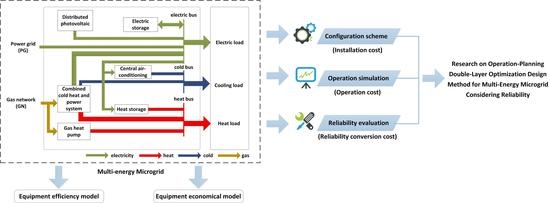
The multi-energy microgrid is an energy system that runs autonomously. The system consists of energy management devices, distributed renewable energy sources, energy storage devices, energy conversion devices, and energy loads; structurally, the microgrid is composed of energy input, conversion, and storage, as well as output components. In this study, a multi-energy microgrid was built based on the energy hub model, which consisting of a combined cold heat and power (CCHP) system, a gas heat pump (GHP), a distributed photovoltaic (PV), central air conditioning (CAC), electric storage (ES), and heat storage (HS) components with power, gas, cold, and heat energies. The structure of the multi-energy microgrid is shown in Figure 1.
The multi-energy microgrid contains various equipment units that couple with each other to meet the needs of different energy loads. Power loads are supplied by the CCHP system and PV. The ES or power grid (PG) make up for insufficient outputs; heat loads are supplied by the CCHP and GHP. HS devices make up for insufficient outputs; cold loads are supplied by the CCHP and CAC. In the case of failure, different forms of energy give priority to the supply of energy loads and supplement of energy storage devices of the same kind. Extra energy can be employed for conversion or backup to reflect the differences among energy grades.
The multi-energy microgrid is an independent and controllable basic unit of the energy Internet at the user terminal. Its flexible operation mode can reduce the energy consumption during transmission and realize the effective consumption of renewable energy sources. The reliability of two typical microgrid system operation modes—the grid-connected mode and the electric-isolated mode—was analyzed to fully consider the reliability factors. Subsequently, a novel planning method for the electric-isolated mode system was proposed. The main assumptions regarding the multi-energy microgrid model are as follows.
(1)
Energy distribution networks are placed into a single bus radiation network structure with a certain level of isolation between the devices in the multi-energy microgrid.
(2)
Different types of energy loads are intensively provided by relevant devices.
(3)
Failure in any one-unit device occurs independently; only single failure is considered [22].

3. Equipment Efficiency and Economical Models

3.1. Gas-Fired CCHP System

The CCHP system, the key unit of the microgrid system, provides energy for internal equipment (e.g., absorption chiller and heat exchanger) and the cooling, heating, and power loads of the microgrid system. Configuration planning of the multi-energy microgrid centers around the CCHP output and fuel consumption. The efficiency model of the gas-fired CCHP system is [23]:
{ Q M T = P o u t p u t C C H P ( 1 η M T C C H P η 1 C C H P ) / η M T C C H P Q h 0 = Q M T η r e c C C H P K h 0 Q c 0 = Q M T η r e c C C H P K c 0 η r e c C C H P = T 1 T 2 T 1 T 0 V M T C C H P = ( P o u t p u t C C H P Δ t ) / ( η M T C C H P L )
where QMT is the exhaust residual heat of the CCHP system; P o u t p u t C C H P is the output power of the CCHP system; η M T C C H P is the efficiency of the gas turbine, which is set as 75%; η 1 C C H P is the heat dissipation coefficient of the CCHP system, which is set as 25%; Qh0 and Qc0 are the heating or refrigerating capacity provided by the residual heat from the gas turbine, respectively; η r e c C C H P is the recovery efficiency of waste heat from flue gas; Kh0 and Kc0 are the heating or refrigerating coefficient of bromine cooler, which are set as 1.2 and 0.95, respectively; T1 and T2 are the environmental coefficients, which are set as 573.15 K and 423.25 K, respectively; V M T C C H P is the amount of natural gas consumed by the CCHP system; L is the low calorific value of natural gas, which is set as 9.7 kW·h/m3; and Δt is the unit run time.
Under Equation (1), the CCHP uses waste heat for heating or cooling. If there are remaining heating and cooling loads to be satisfied, extra gas consumption is necessary during the warming up period [23]; that is:
V h 1 C C H P = ( Q h Q h 0 ) Δ t h K h 0 η i n C C H P L
V c 1 C C H P = ( Q c Q c 0 ) Δ t c K c 0 η i n C C H P L
where V h 1 C C H P and V c 1 C C H P are the amount of natural gas that is needed for heating or refrigeration in the CCHP system; Qh and Qc are the heat or cold load to be satisfied by the CCHP system; η i n C C H P is the operation efficiency of the CCHP for supplementary combustion, which is set as 75%; and Δth and Δtc are operation time of gas turbine in heating or cooling, respectively.
Apart from the inherent installation cost, the fuel cost of the CCHP system can be calculated as follows:
C fuel CCHP = ( w gas / L ) t ( P output CCHP / η MT CCHP )
where C fuel CCHP is the fuel cost of CCHP system; and w gas is natural gas price.
The operation and maintenance costs of the CCHP can be calculated as follows:
C opma CCHP = K MT CCHP t P output CCHP
where C opma CCHP is the operation and maintenance costs of the CCHP system; and K MT CCHP is the proportional coefficient of the CCHP’s operation and maintenance costs.

3.2. Energy Conversion Equipment

The multi-energy microgrid contains several pieces of energy conversion equipment, including the GHP and CAC. Combined with the energy hub model, the efficiency output model of the energy conversion equipment is [2]:
P b ( t ) = C ab P a ( t )
where Cab is the energy conversion coefficient.
Besides the equipment installation cost, operation and maintenance costs also must be considered during the planning phase. The operation and maintenance costs of the energy conversion equipment can be calculated as follows [24]:
C opma Trans ( t ) = Δ t m = 1 N Trans K MT m | P output m ( t ) |
where NTrans is the total number of energy conversion equipment units.

3.3. PV Power Generation System

The output model of the PV system is [25]:
P P V ( t ) = f PV P PV , rated A ( t ) A S [ 1 + α p ( T E M ( t ) T E M STC ) ]
where fPV is the power reduction factor of PV, which is set as 0.9; P PV , rated is the rated power of PV; A(t) is the actual irradiance on the PV current tilt plane; AS is the irradiance under standard test conditions, which is set as 1 kW/m2; αp is the power temperature coefficient, which is set as −0.47%/°C; TEM(t) is the surface temperature of PV; and TEMSTC is the temperature of PV under standard test conditions, which is set as 25 °C in this study.
Unlike other components in the multi-energy microgrid, the PV system does not need primary energy. Thus, no fuel cost is needed. It is much less expensive to operate PV than it is to run other equipment. By fully considering the PV construction cost, maintenance cost, labor cost, price increase indices, government subsidies, the actual service life of the PV system, the net PV residual value, and the unit conversion cost of PV, power generation is calculated to simplify the following economical calculations. The conversion cost is as follows:
C output PV = N PV P PV , rated c PV 0 ( 1 ρ ) + Y PV = 1 N Y , PV f ( Y ) N Y , PV N PV T PV , max M PV B subsidy
where NPV is the number of PVs; cPV,0 is the unit capacity investment in PV construction; ρ is the net residual rate, which is set as 3%; f(Y) is the net residual value of PV; MPV is the installation capacity of PV; and Bsubsidy is the national subsidy for energy-saving and emission reduction, which is set as 0.1 ¥/kW·h.
The net residual value of PV is:
f ( Y ) = ( 1 + β PV ) Y C oper PV
where βPV is the price rise coefficient, which is set as 5%; and Y is the planning life cycle, which is set as 12a.

3.4. ES Devices

The lead–acid batteries (LB) are employed as electric storage devices for the microgrid system that is modeled in this study. Compared with other power storage technologies, the LB features higher charging efficiency and energy density, and it is not constrained by space, so it is a better fit for the microgrid system. The dynamic model is [26]:
S O C ( t ) = ( 1 δ ) S O C ( t 1 ) + P C ES ( t ) Δ t η C ES / E SOC P D ES ( t ) Δ t E SOC η D ES
where SOC(t) is the electric quantity of ES at time interval t; δ is the ES self-discharge rate, which is set as 0.5%/h; P C ES ( t ) and P D ES ( t ) are the charging and discharging power of ES at time interval t, respectively; η C ES and η D ES are the charging or discharging efficiency of ES, which are set as 90% and 90%, respectively; and ESOC is the rated capacity of ES.
LB has a low self-discharge rate, so self-discharge loss is ignored. The cost lost in ES during operation mainly includes the costs of life loss C life ES and power transmission loss C trans ES . The cost of life loss in the power storage device can be calculated as follows:
C life ES = μ ES C invest ES N ( | E S ( t 1 ) E S ( t ) | )
where μ ES is the regulating coefficient of ES, which is set as 1; C invest ES is the one-time ES purchase cost; N(·) is the discharge depth function, which is typically a four-order function that denotes the relationship between cycle life and discharge depth [23]; ES(t) is the power energy proportion of the current LB, which can be calculated as follows:
E S ( t ) = S O C ( t ) E S O C
The power transmission loss C trans ES of ES devices results from incomplete transmission. It can be expressed as follows:
C trans ES ( t ) = c trans ES [ ( 1 η C ES ) P C ES ( t ) + ( 1 / η D ES 1 ) P D ES ( t ) ]
When the multi-energy microgrid system runs in grid-connected mode, ES devices serve to stabilize the fluctuation of renewable energy and improve the economical performance of the system. The charging and discharging states of ES devices are associated with the output of the relevant unit and the electricity pricing mechanism. When the microgrid system runs in electric-isolated mode, the ES devices provide a significant backup energy supply. When something goes awry in the microgrid system, extra power energy will be supplied first to the ES devices and similar types of loads. Energy conversion will be possible if extra energy sources remain.

3.5. HS Devices

The regenerative electric boiler is selected as the HS device in the system model. It not only stores heat; it also helps absorb renewable energy sources. The dynamic model of HS devices is [23]:
H HS ( t ) = ( 1 k LOSS ) H HS ( t 1 ) + Q C HS ( t ) Δ t η C HS Q D HS ( t ) Δ t η D HS
where HHS(t) is the heat of HS at time interval t; kLOSS is the heat dissipation rate of HS, which is set as 1%/h; η C HS and η D HS are the charging and discharging efficiency of HS, which are set as 90% and 90%, respectively.
The circular life loss of the HS devices is smaller than that of the ES devices, and is not considered in this study. The operating cost of the HS device mainly includes the idle cooling cost and heat transmission loss cost. The cost of HS device loss can be calculated as follows:
C oper HS ( t ) = c h 0 H S [ k LOSS H HS ( t 1 ) + ( 1 η C HS ) Q C HS ( t ) Δ t + ( 1 / η D HS 1 ) Q D HS ( t ) Δ t ]

4. Multi-Energy Microgrid Reliability Assessment

Reliability lays the foundation for any ideal planning scheme. As mentioned above, FMEA and Monte Carlo simulation were combined to remedy the problems inherent to extant reliability assessment methods. FMEA was employed to analyze the logical relationship of energy supply in the microgrid system, and quantify the potential effects of unit fault on different types of energy supply. Thus, their various coupling features can be reflected. Monte Carlo simulation is a reliability assessment method that can be applied to the multi-energy supply of the microgrid to simulate the timing sequence features of the equipment units and load demands in the system.
Taking grid-connected operation mode as the example, the reliability status of different energy types (power, heat, and cold) can be calculated as follows:
R elec = f ( S CCHP , S PV , S ES , S PG , S GN ) R heat = f ( S CCHP , S GHP , S HS , S GN ) R cold = f ( S CCHP , S CAC , S GN )
where R is the reliability of an energy supply; f(·) is the calculation function of energy supply reliability; and S(·) is the state of equipment.
Based on the multi-energy microgrid shown in Figure 1, the failures in the CCHP, GHP, CAC, PV, ES, PG, and gas network (GN) of the microgrid system were analyzed. Also, this study divided one year into 8760 one-hour time periods. In each period, the equipment status parameters were kept unchanged, and the instantaneous quantity was recorded at specific time points.

4.1. State Model of Equipment Units

In the microgrid system, the output of units (e.g., PV or CCHP) and different energy load demands have robust time-sequential characteristics. It is challenging to model these characteristics mathematically, which affects the feasibility of any reliability evaluation. A state model of equipment units must be built to simulate the equipment unit states via the Monte Carlo method. Subsequently, the time-sequential characteristics in the microgrid system can be modeled appropriately.
The Markov two-state models [8] were employed to describe the equipment units of the microgrid system. The normal state of a unit is presented in an exponential distribution. The duration from the unit’s normal working state to failure is:
T f , k = ( 1 λ k ) ln u k k [ 1 , 2 , m ]
where λk is the failure rate of kth equipment unit; and uk represents the random numbers of uniform distribution in [0,1] interval.
All of the equipment units are repairable. The failure duration is also an exponential distribution:
T r , k = ( 1 μ k ) ln u k k [ 1 , 2 , m ]
where μk is the repair rate of kth equipment unit.

4.2. Reliability Evaluation Indexes

This study selected the expectation of energy supplied (EES), loss of energy expectation (LOEE), and system average interruption duration index (SAIDI) as the indices to evaluate the reliability of different energy types in the multi-energy microgrid. The multi-energy reliability economic indicator was built by combining energy prices.
(1) EES
This index refers to the probability that a certain energy type reaches the user demand side in a certain period. A higher EES suggests that the energy can meet the demand in the sampling period with high reliability. The specific solution is as follows:
The energy conversion matrix [2] in the energy hub model is extended to the energy transmission power matrix C. Matrix C includes the unit supply matrix CM and adjustable resource matrix CS. The matrix expression forms are shown in Equations (20) and (21). The matrix rows represent different run-time scenarios (including normal operation and failure scenarios); the matrix columns represent the supplies of power, heat, and cold energy types. The unit supply matrix CM refers to the energy output of the unit following the different energy demands in a certain period; the adjustable resource matrix CS refers to the energy provided by backup resources or a utility grid to the microgrid after a certain period. Specific values are associated with specific operation strategies. The energy transmission matrix of the ith scenario in the sampling period is: C i = C M , i + C S , i .
C M = [ P output C C H P + P o u t p u t P V P o u t p u t C C H P + P o u t p u t G H P P o u t p u t C C H P + P o u t p u t C A C P o u t p u t P V P o u t p u t G H P P o u t p u t C A C P o u t p u t C C H P + P o u t p u t P V P o u t p u t C C H P + P o u t p u t G H P P o u t p u t C C H P P o u t p u t C C H P + P o u t p u t P V P o u t p u t C C H P P o u t p u t C C H P + P o u t p u t C A C P o u t p u t C C H P + P o u t p u t P V P o u t p u t C C H P + P o u t p u t G H P P o u t p u t C C H P + P o u t p u t C A C P o u t p u t P V 0 P o u t p u t C A C P o u t p u t C C H P P o u t p u t C C H P + P o u t p u t G H P P o u t p u t C C H P + P o u t p u t C A C P o u t p u t C C H P + P o u t p u t P V P o u t p u t C C H P + P o u t p u t G H P P o u t p u t C C H P + P o u t p u t C A C ]
C S = [ P o u t p u t PG + P o u t p u t ES P o u t p u t HS 0 P o u t p u t PG + P o u t p u t ES P o u t p u t HS 0 P o u t p u t PG + P o u t p u t ES P o u t p u t HS 0 P o u t p u t PG + P o u t p u t ES P o u t p u t HS 0 P o u t p u t ES P o u t p u t HS 0 P o u t p u t PG + P o u t p u t ES P o u t p u t HS 0 P o u t p u t PG + P o u t p u t ES P o u t p u t HS 0 P o u t p u t PG P o u t p u t HS 0 ]
The load energy demand matrix L = [ P L o a d e l e c , P L o a d h e a t , P L o a d c o l d ] reflects the demand for power, heat, and cold energies in the sampling period. The supply and demand comparison matrix Q can be built accordingly. The elements in matrix Q are Boolean variables. The elements Q j , i , k ( j = 1 , 2 , N ; i = 1 , , 8 ; k = e , h , c ) in the matrix represent the j-th sampling, i-th scene obtained, and discrimination of the k-th energy source. The distinguishing method of power energy, e.g., in the matrix is as follows:
Q j , i , e = { 0 P L o a d e l e c > C M , i , e + C S , i , e 1 P L o a d e l e c C M , i , e + C S , i , e
The energy supply expectation of power, heat, and cold energy types in the microgrid are calculated by Equations (23)–(25), respectively:
E E S e l e c = 1 N j = 1 N Q j , i , e
E E S h e a t = 1 N j = 1 N Q j , i , h
E E S c o l d = 1 N j = 1 N Q j , i , c
where N is the number of Monte Carlo simulated sampling time periods.
(2) LOEE
This index denotes the gross loss of energy due to unit failure or outage of a certain energy source in the statistical time period. The unit is MW·h/a. A higher LOEE suggests that the energy source is greatly influenced by unit failure, and that energy supply reliability is low. The index is calculated by Equations (26)–(28).
L O E E e l e c = 8760 T j = 1 N L O E E i e l e c
L O E E h e a t = 8760 T j = 1 N L O E E i h e a t
L O E E c o l d = 8760 T j = 1 N L O E E i c o l d
where T is the evaluation time cycle.
(3) SAIDI
SAIDI refers to the duration of insufficient supply of a certain type of energy caused by unit failure or outage in the statistical time period. The unit is h/a. Longer duration means a larger impact of unit failure and low-energy supply reliability. This index is calculated by Equations (29) and (31):
S A I D I e l e c = 8760 T j = 1 N S A I D I i e l e c
S A I D I h e a t = 8760 T j = 1 N S A I D I i h e a t
S A I D I c o l d = 8760 T j = 1 N S A I D I i c o l d
(4) Energy supply reliability economic indicator
This study determined energy supply reliability economic indicators by calculating the LOEE by type with corresponding prices [27]. The index value reflects the economic loss expectation caused by equipment failure to the multi-energy microgrid system. It is calculated as follows:
C RE = w e l e c L O E E e l e c + w h e a t L O E E h e a t + w c o l d L O E E c o l d
where w e l e c , w h e a t , and w c o l d are the energy loss values of electricity, heat, and cold, respectively. The specific values can be extracted from the references [18].

4.3. FMEA Analysis for Reliability Evaluation

Due to space limitations, this study report here only analyses the impact of CCHP failure as well as quantitative analysis of the complementary coupling relationship between different energy types.
CCHP failure influences the supply of cold, heat, and power energy. Power loads are mainly supplied by the PV, with a backup supplement from ES devices and PG; cold loads are supplied by CAC under the condition that there is extra power energy and that CAC output constraints are satisfied. Heat loads are supplied by the GHP under the condition that the GHP output constraints are satisfied with backup support from HS devices.
Based on the evaluation indexes introduced in Section 4.2, the LOEE can be calculated by Equations (33) and (34):
L O E E C C H P e l e c = k e , C C H P ( λ C C H P L O E E k e , C C H P e l e c )
L O E E k e , C C H P e l e c = { 0 P L o a d e lec ( t ) P o u t p u t ES ( t ) + P o u t p u t P V ( t ) + P o u t p u t EN ( t ) r C C H P [ P L o a d e ( t ) ( P o u t p u t ES ( t ) + P o u t p u t P V ( t ) + P o u t p u t EN ( t ) ) ] d t P L o a d e l e c ( t ) > P o u t p u t ES ( t ) + P o u t p u t P V ( t ) + P o u t p u t EN ( t )
SAIDI can be calculated by Equations (35) and (36):
S A I D I C C H P e l e c = k e , C C H P ( λ C C H P S A I D I k e , C C H P e l e c )
S A I D I k e , C C H P e l e c = { 0 P L o a d e l e c ( t ) P o u t p u t ES ( t ) + P o u t p u t P V ( t ) + P o u t p u t EN ( t ) r C C H P P L o a d e l e c ( t ) > P o u t p u t ES ( t ) + P o u t p u t P V ( t ) + P o u t p u t EN ( t )
where ke,CCHP is the power supply area affected by the fault of the CCHP system.
Likewise, the relevant reliability indexes of heat and cold energy types can be calculated by Equations (37)–(40):
L O E E k h , C C H P h e a t = { 0 P L o a d h e a t ( t ) P o u t p u t G H P ( t ) + P o u t p u t HS ( t ) r C C H P [ P L o a d h e a t ( t ) ( P o u t p u t G H P ( t ) + P o u t p u t HS ( t ) ) ] d t P L o a d h e a t ( t ) > P o u t p u t G H P ( t ) + P o u t p u t HS ( t )
L O E E k c , C C H P c o l d = { 0 { P L o a d elec ( t ) < P o u t p u t ES ( t ) + P o u t p u t P V ( t ) + P o u t p u t EN ( t ) } & { P L o a d c o l d ( t ) < P o u t p u t C A C ( t ) } r C C H P [ P L o a d c o l d ( t ) P o u t p u t C A C ( t ) ] d t { P L o a d e l e c ( t ) < P o u p u t ES ( t ) + P o u t p u t P V ( t ) + P o u t p u t EN ( t ) } & { P L o a d c o l d ( t ) P o u t p u t CAC ( t ) } r C C H P [ P Load c o l d ( t ) ] d t P Load e l e c ( t ) P o u t p u t ES ( t ) + P o u t p u t P V ( t ) + P o u t p u t EN ( t )
S A I D I k h , C C H P heat = { 0 P L o a d h e a t ( t ) P o u t p u t GHP ( t ) + P o u t p u t HS ( t ) r CCHP P L o a d h e a t ( t ) > P o u t p u t GHP ( t ) + P o u t p u t HS ( t )
S A I D I k c , C C H P c o l d = { 0 { P L o a d e l e c ( t ) < P o u t p u t ES ( t ) + P o u t p u t PV ( t ) + P o u t p u t EN ( t ) } & { P L o a d c o l d ( t ) < P o u t p u t CAC ( t ) } { P L o a d e l e c ( t ) < P o u t p u t ES ( t ) + P o u t p u t PV ( t ) + P o u t p u t EN ( t ) } & { P L o a d c o l d ( t ) P o u t p u t CAC ( t ) } r C C H P P Load e l e c ( t ) P o u t p u t ES ( t ) + P o u t p u t PV ( t ) + P o u t p u t EN ( t )
According to the cooling energy determined by Equations (38) and (40), a portion of the cooling loads are supplied by the CAC during normal function. If there is a fault, the system, in terms of energy loads of equal importance, gives priority to electric loads per the higher energy grade of electric power than cooling energy, besides their rigidity and flexibility. In contrast, the cooling loads supplied by the CAC are reduced when a malfunction occurs to ensure the continuous supply of electric loads.
Likewise, the impacts of other unit failures on different energy supplies in the multi-energy microgrid can be analyzed. The effects of PG failures on the microgrid system as well as the supply P o u t p u t PG in the electric-isolated operation mode are not discussed here.

5. Multi-Energy Microgrid Double-Layer Planning Model

The optimized planning model of the multi-energy microgrid has two major parts. First is the optimization at the planning level, which ensures the favorable capacity and quality of energy supply and storage devices in the microgrid system. Second is the optimization at the scheduling level, which serves to optimize the output of power supply devices and the operation of energy storage devices in the microgrid system. Both parts target economical efficiency per the reliability factors of the power supply.

5.1. Optimization Object

In this study, the total cost of the multi-energy microgrid system across its entire life cycle was selected as the target function. The total cost primarily involves the purchase, installation cost, operation cost, and reliability conversion cost. The target function is expressed as:
min { C IN + C OP + C RE }
where CIN is the installation cost; COP is the operation cost; and CRE is the reliability conversion cost.
Where the system construction cost is:
C IN = ( m N m × C inst , m × M m m N m × C scra , m ) r ( 1 + r ) Y ( 1 + r ) Y 1
where Cinst,i is the investment and construction cost of a unit capacity of mth equipment unit; m is the total number of equipment units; and r is the effective rate of interest, which is set as 5%.
The annual operation cost is:
C OP = m t C fuel , m OP ( t ) + C opma , m OP ( t )
where C opma , m OP ( t ) is the operating and maintenance cost of mth equipment unit at time interval t.
The calculation method of the reliability conversion cost CRE is expressed as Equation (32).

5.2. Constraints

(1)
Maximum load constraint: The maximum output capacity of the energy supply equipment configuration must meet the maximum power demand of the microgrid system in power, heating, and cooling loads:
m P o u t p u t , max m ( t ) P Load , max [ · ] ( t )
where P o u t p u t , max m ( t ) is the maximum output power of mth energy supply equipment unit at time interval t; and P Load , max [ · ] ( t ) is the maximum load demand for some kind of energy at time interval t.
(2)
Power balancing constraint: If the energy storage function is ensured, a real-time balance of power/heating/cooling energy supply and demand in the multi-energy microgrid should be achieved:
m P o u t p u t m ( t ) + m P D m ( t ) = P Load [ · ] ( t ) + m P C m ( t )
where P o u t p u t [ · ] ( t ) is the output power of mth energy supply equipment unit at time interval t; P [ C / D ] m ( t ) is the charge or discharge power of mth energy storage equipment unit at time interval t; and P L o a d [ · ] ( t ) is the load demand at time interval t.
(3)
Self-sufficiency probability constraint: The multi-energy microgrid works in electric-isolated mode, so it is crucial in regard to meeting the load demands and operation stability of the system. The self-sufficiency probability of meeting the system load demand in the planning period can be employed to direct the planning and configuration of the microgrid system:
Pr ( m P o u t p u t m ( t ) + m P D m ( t ) P L o a d [ · ] ( t ) ) P s t [ · ]
where P s t [ · ] is the probability of self-sufficiency of a certain type of energy load.
(4)
Operation constraint of power supply equipment: The energy supply equipment of the multi-energy microgrid must meet the rated power and climbing constraints of the equipment during operation.
P o u t p u t , min m P o u t p u t m ( t ) P o u t p u t , max m
Δ P d o w n m P o u t p u t m ( t ) P o u t p u t m ( t 1 ) Δ P u p m
where Δ P d o w n m and Δ P u p m are the climbing power of the mth energy supply component to reduce or increase output power.
(5)
Operation constraint of power storage equipment: The energy storage equipment of the multi-energy microgrid must meet the energy charge/discharge power, and capacity constraints of the equipment during operation:
M min m ( t ) M m ( t ) M max m ( t )
P [ C / D ] m ( t ) P [ C / D ] , max m ( t )
where M max m ( t ) and M min m ( t ) are the maximum or minimum capacity of the mth energy storage equipment unit.

5.3. Multi-Energy Microgrid Planning Process

The planning model of the multi-energy microgrid optimization also has two parts: planning optimization and operation scheduling optimization. The configuration scheme is optimized based on the overall energy load level in the microgrid system under the given constraints. In alternative energy supply and storage equipment, considering Equation (42) and the optimal operation conditions in the system’s whole life cycle, an optimized combination scheme for energy supply devices and energy storage devices of the microgrid system is proposed here with the equipment type and quantity as optimization variables. The planning optimization denotes a non-linear integer programming algorithm that does not readily provide an analytical solution, so this study instead employed the quantum-behaved particle swarm optimization (QPSO) algorithm [28]. Considering that the velocity vectors are usually assumed to be small values during the iterative process of the traditional PSO algorithm, one of the main drawbacks of the traditional PSO algorithm is that the solution of the problem is easy to trap into the local optimum rather than the global optimal. Therefore, in this paper, the QPSO algorithm is employed to avoid this problem. By using the wave function to describe the state of a particle instead of the velocity as in a traditional PSO algorithm, and by improving the dynamic behavior of particles, the solution of the problem can effectively avoid falling into local optimum.
Next, based on the hourly load demand curve in the planning period, the power supply of the microgrid system, the demand profile of the microgrid system, and the operation constraints in the energy supply/storage equipment, an hourly optimization scheduling scheme for each component is built by combining the equipment configuration scheme given in the planning part and taking the start/stop and output of the energy supply and storage equipment. Scheduling optimization denotes a mixed non-linear optimization problem, which can also be solved through the QPSO algorithm. Economical indicators under a certain planning scheme throughout the system’s operation can be obtained at the operation level. Thus, they play an important part in the economical target of microgrid system planning. Optimizing the operation and scheduling level is virtually a sub-planning-level optimization process.
The optimized operation and scheduling level denotes the economic performance of the microgrid system under normal operation conditions. The economical efficiency converted by the energy supply reliability of the microgrid system is also calculated to determine the economic loss expectation produced under fault conditions and improve the economical indexes. This process is illustrated in Figure 2.

6. Case Study

6.1. Case Overview

This study employed a series of typical industrial parks in southern China to validate the proposed method. The physical structure and equipment composition of the microgrid system is given in Figure 1. In regard to energy supply and demand, April to October are classified as cooling months (i.e., with large demand for cooling loads). Heating loads include the demand for drying and ventilation during the production and hot water for residential life; they have no definite supply period, but still show some seasonal characteristics. There are demands for electric loads throughout the year.
Curves reflecting the demands for electric, heating, and cooling loads in the microgrid system throughout the year are shown in Figure 3. The available types of energy production/conversion equipment and economical operating parameters in the microgrid based on the above demands are listed in Table 1; the types and economical operating parameters of energy storage devices are listed in Table 2. The initial capacities of ES and HS are 30% and 50% of the rated capacity, respectively; the maximal charge–discharge power is 80% of the rated capacity [29]. The reliability parameters of various equipment units are listed in Table 3.
The gas network sets the fault rate and repair time of the main gas pipeline. Various factors correlated with power-generating efficiency are discussed here. The installed capacity of the PV is 4.6 MW; the annual output curve is shown in Figure 4. The optimization of different PV configurations is not discussed in subsequent planning programs. According to the local power pricing policy, the power price peaks at 11:00–15:00 and 19:00–21:00, and then valleys at 0:00–7:00; in other periods, the price remains stable. Table 4 lists the prices for different energy types. The loss value of electric/heating/cooling loads in the microgrid are 200 ¥/kW·h, 120 ¥/kW·h, and 120 ¥/kW·h, respectively. Self-sufficiency probability is 90%.

6.2. Configuration of Storage Devices

The microgrid system described in this study operates in electric-isolated mode and in a self-sufficient manner. The overall time cycle of the scheme is planned to be 10 years, i.e., Y = 10a. The 10th year is considered the target year. It is also assumed that installation occurs in the first year of the planning horizon [30]. The penalty coefficient of the relevant algorithms is 0.03, the population scale is 80, the inertia factor is 0.5, the self factor is 2, the global factor is 2, the mutation probability is 0.05, the iteration number N is 1000, and the error precision σ is 0.01. Four different cases were employed to analyze the impacts of different configurations on the selection and reliability of different microgrid planning schemes.
  • Case 0: A microgrid system without ES or HS devices;
  • Case 1: A microgrid system with HS devices but lacking ES devices;
  • Case 2: A microgrid system with ES devices but lacking HS devices;
  • Case 3: A microgrid equipped with both ES and HS devices.
This study calculated the optimal configuration scheme according to the above four cases; see Table 5 and Table 6 for their respective results and costs. Case 3 has the best economical performance considering the capacity, configuration, operation, and reliability of the microgrid system. Case 0 has low investment costs, as it lacks energy storage devices. In this case, the energy supply equipment of the microgrid system is forced to meet the load demands at any moment and deal with the intermittency of distributed PV power, resulting in high operation costs. The absence of energy storage devices also leads to low reliability, especially when malfunction occurs, which increases the loss expectation.
Cases 1 and 2 have different energy storage devices. The HS device is a pure backup resource that improves heating reliability. The ES device can stabilize the volatility of PV, which can improve the microgrid system’s power supply reliability and further enhance the reliability of other energy resources by using the energy conversion devices. Accordingly, the ES device is more important than the HS device.

6.3. Reliability Assessment

Reliability is an important indicator for any ideal planning configuration scheme. Therefore, this study carefully assessed the reliability of the energy supply to the system based on the above optimized configuration scheme. The energy supply reliability of the microgrid system under different cases were compared per the reliability indicators discussed in Section 4.2. The calculation results are shown in Table 7 and Figure 5 and Figure 6.
In Case 1, the system lacks the backup of energy storage devices and meets energy demands through the cooperation of relevant equipment units within the microgrid system. The distributed PV power with high volatility cannot be stabilized effectively. Accordingly, energy supply reliability is poor under random fault due to the lower degree of coupling among energy sources. A reasonable configuration of energy storage devices in the microgrid can effectively stabilize the output randomness of renewable energy sources, reduce the capacity redundancy of the energy production devices, improve the energy supply reliability, and ensure an economical system performance. The HS device is a backup resource that is critical for heat supply reliability. The ES device not only improves the reliability of the power supply, it also converts energy sources through CAC when necessary. Power storage devices improve the coupling among energy sources in the microgrid system and indirectly enhance the energy supply reliability of other energy sources in the system.
Typical optimal configuration schemes under Case 4 were selected for further analysis in accordance with their favorable annual reliability. Preconceived CCHP faults were simulated to explore the impacts on all of the power, heating, and cooling resources with multi-energy coupling on energy supply reliability under different energy demands. This study selected the peak and valley periods of power loads, heat loads, and cold loads in a typical year, simulated CCHP outage and failure, and then evaluated the LOEE and outage impact time expectation (re) of the multi-energy microgrid under different energy demands. A pre-arranged outage time according to the reference value of failure repair, 24 h, was employed to ensure that the expected failure time did not affect the results. The evaluations are listed in Table 8, where e-peak, h-peak, and c-peak denote the peak periods of power loads, heat loads, and cold loads, respectively; likewise, the valley periods of loads are represented.
When performing pre-arranged outage maintenance of a traditional single energy network, the goal is typically to avoid load peaks. However, the comparison of reliability indexes at different typical periods under the same operation mode suggests that although the pre-arranged valley outage value does partially ensure sufficient energy supply, it significantly impacts other energy supplies under multi-energy coupling and energy supply cycle circumstances. The valley value of power loads may actually have a greater impact on cold loads than the simulated peak failure value.
On this basis, the energy supply reliability economic indicator was further analyzed to determine the optimal maintenance time for major equipment in the microgrid system. Through the calculation, the preconceived accident simulation is conducted at the moment t = 3500, and can get Imin = 1332.631 CNY. On account of the high PV output in the simulation period, ES can effectively reduce the loss of energy supply. Extra power can be employed for cold loads through CAC, and heat loads can be transferred completely through GHP. Hence, the influence on the microgrid system at this moment is lower than that of other moments.

6.4. Discussions

In the case study, this study quantitatively analyzed the influence of different equipment configuration schemes on the economy and reliability of multi-energy microgrid planning from different perspectives. On the basis, the reliability of a pre-scheduled outage in a typical scene was analyzed, and a kind of application scenario of reliability evaluation was put forward. The results of the cases are discussed as follows:
(1)
According to the analysis of Section 6.2, although energy storage equipment will increase the installation cost of the microgrid system to some extent, energy storage equipment can stabilize the volatility of the renewable energy output and optimize energy distribution. Therefore, the operation cost of the microgrid system is improved, and the energy storage equipment can play the role of a backup resource, which enhances the reliability of the microgrid system. Considering the reliability conversion cost, the configuration of the energy storage equipment can improve the total cost of the microgrid system.
(2)
The analysis of Section 6.3 suggests that compared with ES, HS equipment can only play the role of heat energy reserve resources, so the contribution to reliability promotion is limited. The ES equipment can not only provide support for improving the reliability of a power supply, it can also indirectly enhance the reliability of the cooling supply because of the coupling characteristics of the multi-energy networks through the equipment.
(3)
Based on the analysis of the reliability of the multi-energy microgrid system, the reliability within a pre-arranged outage in a typical scene was further analyzed in Section 6.3, which can be referenced by the establishment of a maintenance strategy for key equipment in a microgrid system.

7. Conclusions

This study took a multi-energy microgrid as its research target, sorted out the energy efficiency and economical models of the key equipment in the microgrid system, presented a double-layer model with optimal configuration, operation, and reliability consideration for the multi-energy microgrid planning, and determined the optimal capacity configuration and energy management scheme via an optimization algorithm. Compared with traditional, independently supplied and operated energy supply methods, joint planning and design considering multi-energy coupling and complement significantly improved the economic performance of the microgrid system. The energy storage device in the microgrid system mitigated fluctuations in the output of distributed power and further enhanced the energy supply reliability of the microgrid.
In the meantime, this study also proposed a calculation method for energy supply reliability under multi-energy circumstances and perfected the planning model in terms of the economic loss caused by reliability evaluations. The study properly calculated the significance of reliability in planning and compensated for drawbacks in the traditional planning model (which only considers economical factors under normal operation). The optimized design model with the noted reliability consideration can help decision-makers determine the optimal equipment capacity and quantity to satisfy the load demands in actual multi-energy microgrids. The proposed model was designed to not only improve energy supply reliability, but also minimize cost. On this basis, the paper further studied the function of reliability in the maintenance of key units. Based on the proposed reliability assessment techniques, the paper made a comprehensive analysis on the planning, operation, and maintenance of a multi-energy microgrid, providing certain guidance for the future construction of integrated energy systems.
For future research, regarding reliability evaluation, the impact of the system structure such as lines, pipelines on reliability, as well as the time-delay difference of different energy transmission will be further considered. Moreover, the impact of different operation modes of a microgrid system on reliability will be analyzed as well. In the research on planning methods, energy efficiency, pollutant emissions, and other factors will be further considered to improve the planning model from different perspectives.

Author Contributions

Conceptualization, S.G., J.L. and H.L.; methodology, J.L. and H.L.; J.L. and H.S.; validation, S.G. and H.L.; formal analysis, J.L.; writing—J.L. and Y.W.; writing—review and editing, S.G. and H.L.

Funding

This research was funded by National Natural Science Foundation of China, grant number 51777133.

Acknowledgments

This work was supported by the National Key R&D Plan of China (2017YFB0903400).

Conflicts of Interest

The author’s team has confirmed that there is no conflict of interest in this paper.

References

  1. Lin, W.; Jin, X.; Mu, Y.; Jia, H.; Xu, X.; Yu, X.; Zhao, B. A two-stage multi-objective scheduling method for integrated community energy system. Appl. Energy 2018, 216, 428–441. [Google Scholar] [CrossRef]
  2. Geidl, M.; Koeppel, G.; Favre-Perrod, P.; Klöckl, B.; Andersson, G.; Fröhlich, K. Energy hubs for the future. IEEE Power Energy Mag. 2007, 5, 24–30. [Google Scholar] [CrossRef]
  3. Wu, J.; Yan, J.; Jia, H.; Hatziargyriou, N.; Djilali, N.; Sun, H.B. Integrated Energy Systems. Appl. Energy 2016, 167, 155–157. [Google Scholar] [CrossRef]
  4. Razeghi, G.; Gu, F.; Neal, R.; Samuelsen, S. A generic microgrid controller: Concept, testing, and insights. Appl. Energy 2018, 229, 660–671. [Google Scholar] [CrossRef]
  5. Liu, T. Energy management of cooperative microgrids: A distributed optimization approach. Int. J. Electr. Power Energy Syst. 2018, 96, 335–346. [Google Scholar] [CrossRef]
  6. Li, H.; Eseye, A.T.; Zhang, J.; Zheng, D. Optimal energy management for industrial microgrids with high-penetration renewables. Prot. Control Mod. Power Syst. 2017, 2, 1–12. [Google Scholar] [CrossRef]
  7. Escalera, A.; Hayes, B.; Prodanović, M. A survey of reliability assessment techniques for modern distribution networks. Renew. Sustain. Energy Rev. 2018, 91, 344–357. [Google Scholar] [CrossRef]
  8. Billinton, R.; Wang, P. Teaching distribution system reliability evaluation using Monte Carlo simulation. IEEE Trans. Power Syst. 1999, 14, 397–403. [Google Scholar] [CrossRef]
  9. Che, L.; Zhang, X.; Shahidehpour, M.; Alabdulwahab, A.; Abusorrah, A. Optimal Interconnection Planning of Community Microgrids with Renewable Energy Sources. IEEE Trans. Smart Grid 2017, 8, 1054–1063. [Google Scholar] [CrossRef]
  10. Xu, X.; Mitra, J.; Wang, T.; Mu, L. An Evaluation Strategy for Microgrid Reliability Considering the Effects of Protection System. IEEE Trans. Power Deliv. 2016, 31, 1989–1997. [Google Scholar] [CrossRef]
  11. Chen, C.; Wu, W.; Zhang, B.; Singh, C. An Analytical Adequacy Evaluation Method for Distribution Networks Considering Protection Strategies and Distributed Generators. IEEE Trans. Power Deliv. 2015, 30, 1392–1400. [Google Scholar] [CrossRef]
  12. Moeini-Aghtaie, M.; Farzin, H.; Fotuhi-Firuzabad, M.; Amrollahi, R. Generalized Analytical Approach to Assess Reliability of Renewable-Based Energy Hubs. IEEE Trans. Power Syst. 2016, 32, 368–377. [Google Scholar] [CrossRef]
  13. Li, G.; Bie, Z.; Kou, Y.; Jiang, J.; Bettinelli, M. Reliability evaluation of integrated energy systems based on smart agent communication. Appl. Energy 2016, 167, 397–406. [Google Scholar] [CrossRef]
  14. Koeppel, G.; Andersson, G. Reliability modeling of multi-carrier energy systems. Energy 2009, 34, 235–244. [Google Scholar] [CrossRef]
  15. Koeppel, G.; Andersson, G. The influence of combined power, gas, and thermal networks on the reliability of supply. In Proceedings of the Sixth World Energy System Conference, Torino, Italy, 10–12 July 2006; pp. 646–651. [Google Scholar]
  16. Chaudry, M.; Wu, J.; Jenkins, N. A sequential Monte Carlo model of the combined GB gas and electricity network. Energy Policy 2013, 62, 473–483. [Google Scholar] [CrossRef]
  17. Adefarati, T.; Bansal, R.C. Reliability and economic assessment of a microgrid power system with the integration of renewable energy resources. Appl. Energy 2017, 206, 911–933. [Google Scholar] [CrossRef]
  18. Shahmohammadi, A.; Moradi-Dalvand, M.; Ghasemi, H.; Ghazizadeh, M.S. Optimal Design of Multicarrier Energy Systems Considering Reliability Constraints. IEEE Trans. Power Deliv. 2015, 30, 878–886. [Google Scholar] [CrossRef]
  19. Al Ghaithi, H.M.; Fotis, G.P.; Vita, V. Techno-economic assessment of hybrid energy off-grid system—A case study for Masirah island in Oman. Int. J. Power Energy Res. 2017, 1, 103–116. [Google Scholar] [CrossRef]
  20. Rana, M.M.; Xiang, W.; Wang, E. Smart grid state estimation and stabilisation. Int. J. Electr. Power Energy Syst. 2018, 102, 152–159. [Google Scholar] [CrossRef]
  21. Zhang, X.; Shahidehpour, M.; Alabdulwahab, A.; Abusorrah, A.M. Optimal Expansion Planning of Energy Hub with Multiple Energy Infrastructures. IEEE Trans. Smart Grid 2015, 6, 2302–2311. [Google Scholar] [CrossRef]
  22. Conti, S.; Nicolosi, R.; Rizzo, S.A. Generalized Systematic Approach to Assess Distribution System Reliability with Renewable Distributed Generators and Microgrids. IEEE Trans. Power Deliv. 2012, 27, 261–270. [Google Scholar] [CrossRef]
  23. Zhao, B. Key Technology and Application of Microgrid Optimal Configuration; Science Press: Beijing, China, 2015. [Google Scholar]
  24. Dou, C.X.; Liu, B. Multi-Agent Based Hierarchical Hybrid Control for Smart Microgrid. IEEE Trans. Smart Grid 2013, 4, 771–778. [Google Scholar] [CrossRef]
  25. Korkas, C.D.; Baldi, S.; Michailidis, I.; Kosmatopoulos, E.B. Occupancy-based demand response and thermal comfort optimization in microgrids with renewable energy sources and energy storage. Appl. Energy 2016, 163, 93–104. [Google Scholar] [CrossRef] [Green Version]
  26. Zhong, W.; Xie, K.; Liu, Y.; Yang, C. Auction Mechanisms for Energy Trading in Multi-Energy Systems. IEEE Trans. Ind. Inform. 2017, 14, 1511–1521. [Google Scholar] [CrossRef]
  27. Xu, X.; Hou, K.; Jia, H.; Yu, X. A reliability assessment approach for the urban energy system and its application in energy hub planning. In Proceedings of the IEEE Power & Energy Society General Meeting, Denver, CO, USA, 26–30 July 2015. [Google Scholar]
  28. Mohanty, C.P.; Mahapatra, S.S.; Singh, M.R. An intelligent approach to optimize the EDM process parameters using utility concept and QPSO algorithm. Eng. Sci. Technol. Int. J. 2017, 20, 552–562. [Google Scholar] [CrossRef]
  29. Erdinc, O. Economic impacts of small-scale own generating and storage units, and electric vehicles under different demand response strategies for smart households. Appl. Energy 2014, 126, 142–150. [Google Scholar] [CrossRef]
  30. Farret, F.A.; Simões, M.G. Integration of Alternative Sources of Energy; Wiley: Hoboken, NJ, USA, 2006. [Google Scholar]
Figure 1. Structure of multi-energy microgrid.
Applsci 08 02062 g001
Figure 2. Optimal planning process of a multi-energy microgrid.
Applsci 08 02062 g002
Figure 3. Load demand curve.
Applsci 08 02062 g003
Figure 4. Photovoltaic (PV) output curve.
Applsci 08 02062 g004
Figure 5. Comparison of loss of energy expectation (LOEE) in different scenes.
Applsci 08 02062 g005
Figure 6. Comparison of system average interruption duration index (SAIDI) in different cases.
Applsci 08 02062 g006
Table 1. Types and parameters of alternative energy production/conversion equipment. CCHP: combined cold heat and power, GHP: gas heat pump, CAC: central air conditioning.
Devices TypesCapacity/kWInitial Investment Cost/(CNY·kW−1)Operation and Maintenance Cost/(CNY·kW−1)Energy Conversion EfficiencyUpper Limit/kWLower Limit/kW
CCHP 1120047801.5581120012
CCHP 2150047001.5541150015
CCHP 3200045901.5471200020
CCHP 4300035001.4991300030
GHP 180024300.4080%8008
GHP 2100022300.4080%100010
GHP 3150016800.4080%150015
CAC 114005110.3088%140014
CAC 220004600.3090%200020
Table 2. Type and parameters of energy storage equipment. ES: electric storage, HS: heat storage.
Device TypeCapacity/kWInitial Investment Cost/(CNY·kW−1)Operation and Maintenance Cost/(CNY·kW−1)Initial Capacity/kW·hMaximum Power/kW
ES 110007000.03300800
ES 230005800.0310002400
HS10004500.03500800
Table 3. Reliability parameters. PV: photovoltaic, GN: gas network.
Devices Namesλk (f/a)rk (h)
CCHP424
GHP0.62
CAC0.42
PV0.420
ES0.0550
GN0.920
Table 4. Different energy prices.
Types of EnergyEnergy Prices
CNY/kW·h; CNY/m3
electricityPeak period0.80
Waist period0.50
Valley period0.20
gas2.28
Table 5. Optimal configuration of microgrid system.
CaseCCHPGHPCACESHS
0CCHP 4GHP 3CAC 2--
1CCHP 4GHP 2CAC 2-HS
2CCHP 3GHP 2CAC 2ES 2-
3CCHP 3GHP 2CAC 2ES 2HS
Table 6. Cost calculation result. Unit: CNY.
CaseTotal CostCINCOPCRE
08.103 × 1061.805 × 1064.093 × 1062.204 × 106
17.165 × 1061.826 × 1064.126 × 1061.213 × 106
26.464 × 1061.824 × 1063.9 × 1060.757 × 106
36.028 × 1061.880 × 1063.451 × 1060.696 × 106
Table 7. Comparison of expectation of energy supplied (EES) in different cases.
CaseElectricityHeatCold
00.99560.99530.9937
10.99770.99790.9963
20.99850.99740.9972
30.99870.99820.9977
Table 8. Reliability indexes of a typical period of time for the microgrid system. LOEE: loss of energy expectation, re: outage impact time expectation.
Reliability Indexese-Peake-Valleyh-Peakh-Valleyc-Peakc-Valley
LOEE (MW·h)electricity1.9851.79421.4341.1871.8832.482
heat000.129000.959
cold3.8475.1381.6293.9955.0090.047
re (h)electricity182112121618
heat0050010
cold212418232421

