Experimental Study on Vortex-Induced Vibration of Risers Considering the Effects of Different Design Parameters

Abstract

Risers are an indispensable component of offshore oil and gas exploitation structures, and they are vulnerable to vortex-induced vibration (VIV). Although many studies have been conducted to investigate the VIV characteristics of risers, the effects of combination of multiple parameters and the relative significance of each parameter on the risers’ VIV characteristics have rarely been considered. In this paper, 36 experimental cases were investigated to study the risers’ VIV characteristics due to the combination of multiple parameters. The natural frequencies, response microstrains and frequencies of VIV for the risers were obtained. Meanwhile, the effect of each parameter and the relative significance of these parameters on the amplitude of VIV in risers were calculated using grey relational analysis (GRA). The results show that all the parameters considered—i.e., material property (modulus and density), end condition, top tension force and flow velocity—affect risers’ VIV response, and the grey relational grade of these parameters are: $r_{02\left(\mathrm{velocity}\right)}>r_{04\left(\mathrm{constraints}\right)}>r_{05\left(\mathrm{density}\right)}>r_{03\left(\mathrm{tension}\right)}>r_{01\left(\mathrm{modulus}\right)}$.

1. Introduction

Risers are an indispensable component of offshore oil and gas exploitation structures, connecting the wellhead at the sea bottom and the offshore platform at sea surface, and they are utilized to transport the exploited oil and gas (production riser) or to guide the drilling equipment (drilling riser). Nowadays, high-grade steel risers predominate. However, in order to exploit resources in deeper water and harsher environments, different risers are being produced using different materials, such as aluminum (Al) risers, titanium (Ti) risers and fiber-reinforced polymer (FRP) composite risers.

For the Al riser and the Ti riser, the design process and working conditions are similar to those of high-grade steel risers, since all their materials are isotropic. In contrast, FRP composite risers, which are a laminated structure with anisotropic materials, have a different design process and design considerations [1,2]. Many studies, including static analysis and testing, dynamic response, durability under working condition, and so on, have been conducted since the 1950s [3] on the most traditional risers. In the 1980s, the concept of FRP composite risers appeared [4], and since then, more studies and projects have been conducted, such as static and fatigue tests [5,6], verification field tests [7], and pressure integrity tests [8], as well as studies about the optimized design of FRP composite risers by considering the possibilities of different design methodologies, different materials for liner and composite laminate, different laminate stacking sequences, different reinforced fiber angles and different lamina thicknesses [1,2,9,10,11,12].

Compared to other structures, risers are vulnerable to vortex-induced vibration (VIV), i.e., the motions induced on risers interacting with an external flow, which is the main cause of fatigue failure in risers. For metal risers, studies of VIV have been conducted for more than four decades using laboratory and field tests and experiments [13,14,15,16,17]. In addition to the riser (the vertical pipeline), the VIV of the flexible pipeline lying parallel to the bottom floor were also investigated, and the effects of sea-bottom proximity under steady flow and/or wave-induced current on the fatigue life and VIV amplitude and frequency of suspended spans of flexible pipelines were discussed [18,19,20,21]. Meanwhile, the framework for the theoretical analysis of VIV for risers was firstly built by Hartlen and Gurrie (the lift-oscillator model) [22], and this model was then developed for flexible risers [23]; more recently, wake oscillator models were modified and developed according to different parameters and situations [24,25,26,27,28,29]. Currently, computational fluid dynamics (CFD) with different models and methodologies has been applied to solve the VIV problems of risers [17,30,31]. In contrast, for FRP composite risers, the studies of VIV response were comparatively fewer, but still produced inspired results. A global-local analysis methodology was built to investigate the VIV responses of composite risers under semi-empirical fluid load models [32]; Huang and Chen et al. compared the dynamic performance of composite and steel risers using ABQUS and SHEAR7 [33,34], and Wang et al. [35] simulated the VIV response for FRP composite risers by CFD with different modeling methods.

From the previous studies, the VIV of specific risers with fixed design factors were understood, as well as the effect of single design variable on their response for VIV. However, the combination of multiple parameters and the significant sequence of each parameter on risers’ VIV characteristics have rarely been considered. To explore the significant sequence of different parameters on risers’ VIV characteristics, grey relational analysis (GRA) is an effective tool which is small sample, small amount of calculation and no requirement for independency [36]. GRA is an analysis method proposed in grey system theory [37,38] which is based on geometrical mathematics, and it has been successfully employed many engineering fields to solve complicated interrelationships between multiple factors and variables [39,40,41].

GRA is utilized to determine the relational grade between the reference sequence (VIV amplitude in this study) and a given set of parameters (5 design parameters in this study). Then the comparatively best one can be found by comparing the resultant relational grades, i.e., GRA can be regarded as a measure of similarity for finite sequences. The main procedure of GRA includes the following steps: (1) grey relational generation—more specifically, reference sequence and variable sequences are generated using Equation (1), and then these sequences are normalized to comparability sequences using Equation (2); (2) grey relational coefficient calculation—grey relational coefficient is calculated using Equations (3)–(7) and is utilized to determine how close each variable sequence is to its reference sequence (the larger the grey relational coefficient, the closer variable sequence to its reference sequence); and (3) grey relational grade calculation— using the grey relational coefficients in step 2, the grey relational grade between the reference sequence and every variables sequences can be calculated by Equation (8), and when a variable sequence has the highest grey relational grade, this variable has the most significant influence.

In this paper, the experimental study of risers with combined multiple parameters (material property (modulus and density), end condition, top tension force and flow velocity) were conducted to investigate the VIV response. 36 experiment cases are carried out and the natural frequencies, response microstrains and frequencies of VIV for the risers are obtained. In the end, the effect of each parameter and the grey relational grade of these parameters on the amplitude of VIV for riser is calculated using grey relational analysis (GRA).

2. Setup of Experiment

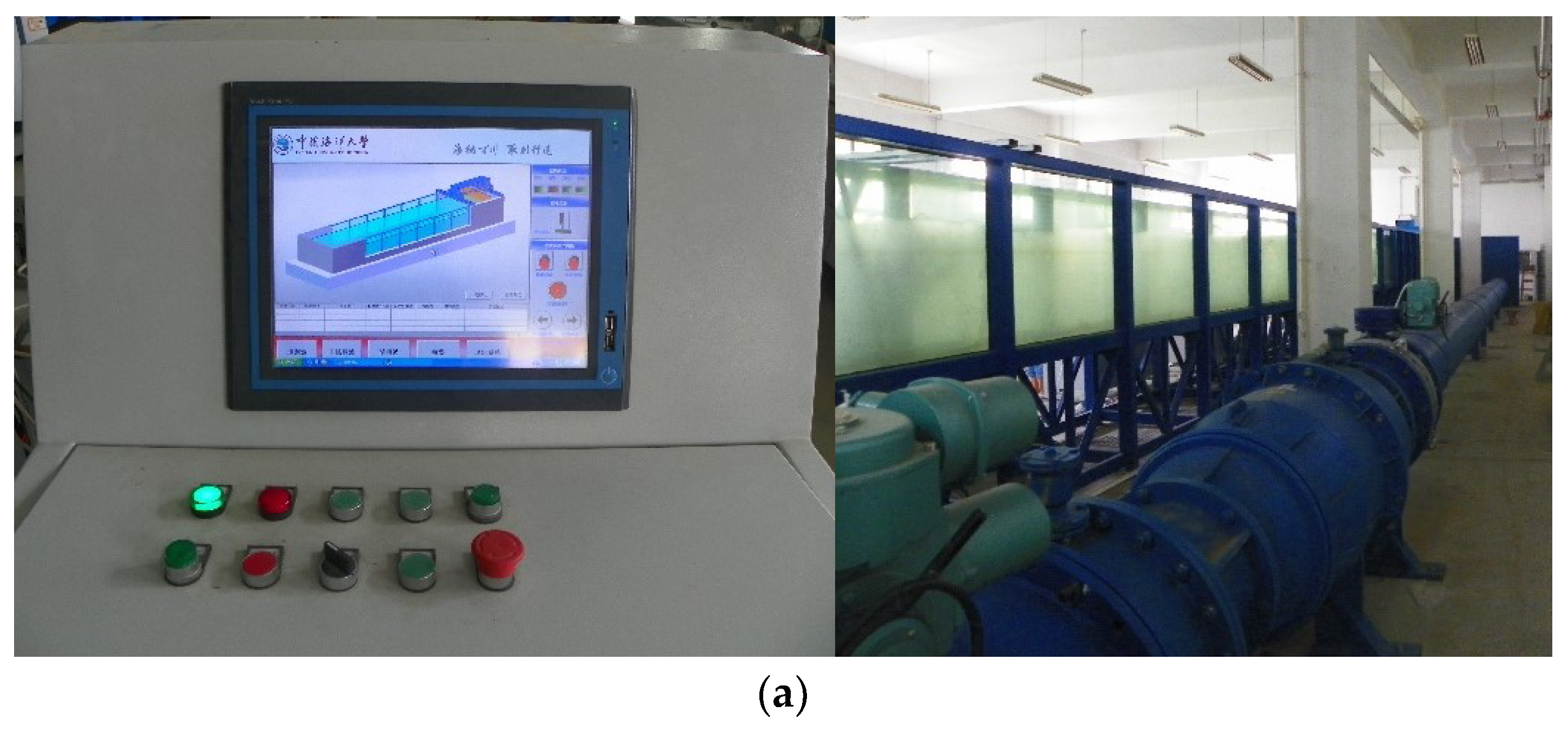
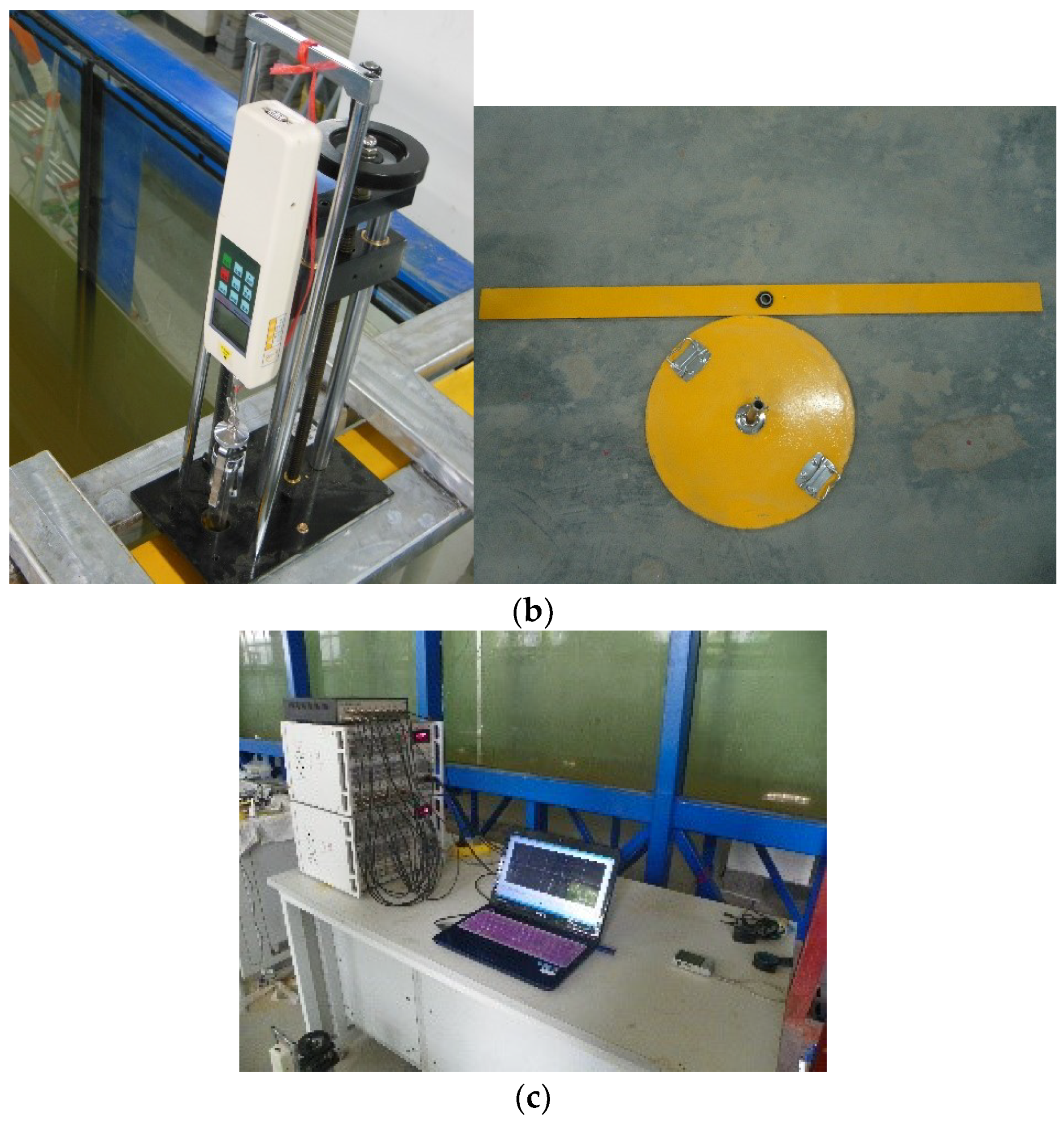
2.1. Instrumentation

The experimental study was conducted using the combined wave-current-wind tank, which is 50 m in length, 1 m in width and 1.2 m in height, in the hydrodynamics laboratory at the Ocean University of China. The testing instrumentation (Figure 1) consists of the following parts: (a) current generation system; (b) velocity monitoring system; (c) end condition system, and (d) data acquisition system. More specifically, the current generation system is utilized to create a uniform flow in the water tank, and the velocity of the current that can be generated ranges from 0 m/s–1.4 m/s, with an accuracy of 5% for the velocity generated. In this study, current velocities of 0.2 m/s, 0.6 m/s and 1.0 m/s are employed. Here we have to note that the riser model is located at the middle part of the water tank in order to ensure that the current velocity is steady at this location. Therefore, the current velocity generated might be different from that at the riser location due to friction. To avoid this, the velocity of the current at the riser location is measured by Nortek Vectrino profiler, and the data is used as feedback to adjust the uniform velocity. The Nortek Vectrino profiler is placed 1 m ahead of the riser model to avoid its influence. The velocity range that can be measured by the Nortek Vectrino profiler is ±0.03 m/s to 4 m/s, and the accuracy is ±0.5% of the measured value of ±1 mm/s. The end condition system is employed to apply top-tension force (ALIYIOI digital force gauge, ALX bracket and special fixture) using a simple support at top and simple/fixed support at bottom (self-made holders). The ALIYIOI digital force gauge is connected to the riser model with its special fixture, and it measures up to 200 N with a resolution of 0.1 N. The accuracy of this force gauge is ±0.5% of the measured value. To provide a simple support at the top and a simple/fixed support at bottom, self-made holders are utilized. For the simple support, a hollow metal ball outside and a solid metal ball inside with a connector to the riser are manufactured; for the fixed support, the connector to the riser is welded to the base plate directly. The data acquisition system is composed of electric resistance strain gauges on the riser model: a SDY2102E dynamic strain indicator and a WS-5921/U60532 supervisory control and data acquisition (SCADA). The resistance value, sensitivity factor and strain limit of the electric resistance strain gauges used are 120 ± 1 Ω, 2.0 + 1% and 20,000 um/m. SDY2102E dynamic strain indicator has 16 channels with bridge resistance of 60 Ω to 1 kΩ. The frequency response of SDY2102E is from DC to 10 kHz (200 Hz is selected in this study) and the sensitivity is 1 V/100 με. WS-5921/U60532 supervisory control and data acquisition has 32 channels with a sampling frequency of 500 kHz, which is utilized to transfer the dynamic strain response of riser model to the Vib’SYS software for further analysis. In this study, 40 s is set as the time range.

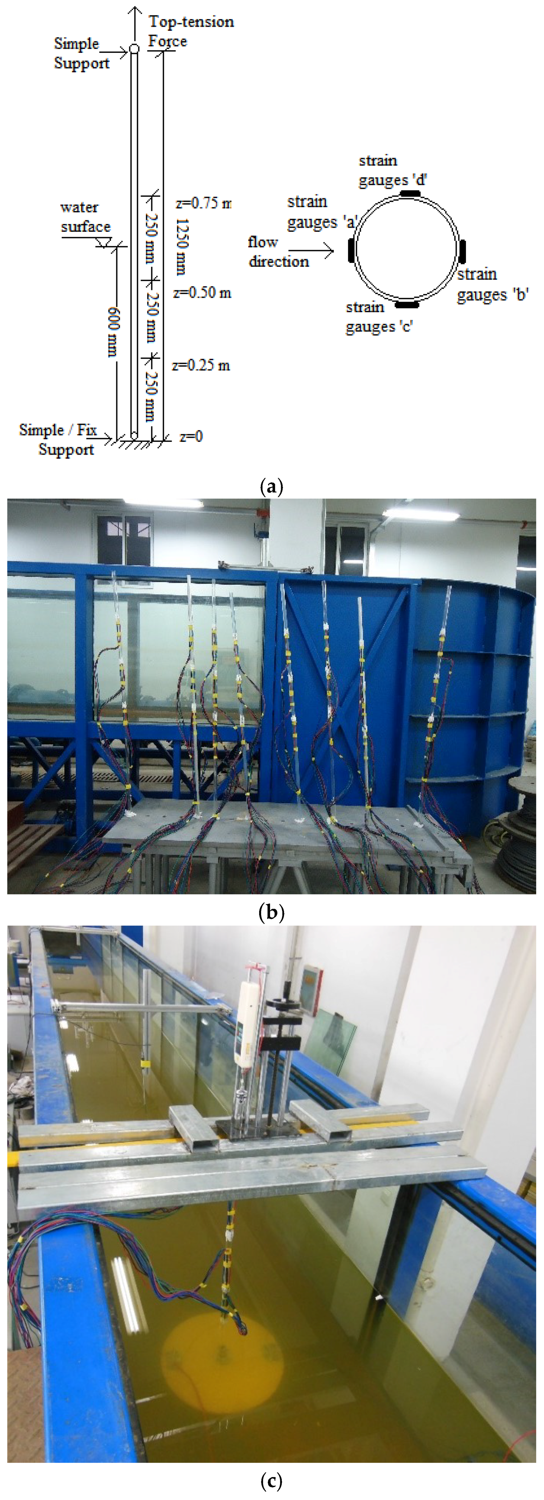
2.2. Experimental Model of Risers

The full-size field testing of risers has extreme requirements in terms of test equipment, time, cost, space and safety, and it is impossible to achieve in any laboratory. Therefore, a scale model is employed whose ratio of length to outer diameter is 62.5; more specifically, the length of the riser model in the test is 1.25 m, with an inner diameter (I.D.) and outer diameter (O.D.) of 0.016 m and 0.02 m, respectively.

The locations of electric resistance strain gauges and the properties of the model risers are presented in Figure 2 and

Table 1. Geometries and properties of the risers.

No.	Materials		O.D. (m)	I.D. (m)	Length (m)	Density (kg/m−3)	Modulus (Pa)
1	Al		0.02	0.016	1.25	3043.17	70 × 109
2	PMMA		0.02	0.016	1.25	1549.89	3.5 × 109
3	UPVC		0.02	0.016	1.25	1153.57	2.0 × 109

. Figure 2a shows the sketch map of the model riser, Figure 2b shows the risers used in the experiment, and Figure 2c shows the holistic test setup for the riser.

The depth of the water is 0.6 m and electric resistance strain gauges are placed at z = 0.25 m, z = 0.50 m and z = 0.75 m (z = 0 is the bottom of the riser), respectively. At each location, 4 strain gauges are employed around the riser’s outer surface (12 strain gauges in total for each riser model).

The geometries and properties of the risers utilized in the experiment are presented in Table 1.

2.3. Experiment Cases

The parameters considered in this paper are the materials for the risers, velocities of flow, end conditions and top-tension forces. The values for each parameter are summarized in

Table 2. Values for each parameter used in the experiment.

Materials	Top Tension Force (N)	End Conditions	Velocities (m/s)
Al/PMMA/UPVC	5/65	S-S/S-F	0.2/0.6/1.0

. As can be seen in Table 2, Aluminum, Poly(methyl methacrylate) (PMMA) and Unplasticized Polyvinyl Chloride (UPVC) are selected as the materials of the riser model; 5 N and 65 N are employed for the top tension force; simple support at top-simple support at bottom (S-S) and simple support at top-fix support at bottom (S-F) are chosen for the end conditions; the flow velocities considered are 0.2 m/s, 0.6 m/s and 1.0 m/s.

According to the values in Table 2, there are 36 experiment cases in total, as presented in

Table 3. Experiment cases.

No.	Parameters	No.	Parameters	No.	Parameters
1	Al, 5 N, S-S, 0.2 m/s	2	Al, 5 N, S-S, 0.6 m/s	3	Al, 5 N, S-S, 1.0 m/s
4	Al, 5 N, S-F, 0.2 m/s	5	Al, 5 N, S-F, 0.6 m/s	6	Al, 5 N, S-F, 1.0 m/s
7	Al, 65 N, S-S, 0.2 m/s	8	Al, 65 N, S-S, 0.6 m/s	9	Al, 65 N, S-S, 1.0 m/s
10	Al, 65 N, S-F, 0.2 m/s	11	Al, 65 N, S-F, 0.6 m/s	12	Al, 65 N, S-F, 1.0 m/s
13	PMMA, 5 N, S-S, 0.2 m/s	14	PMMA, 5 N, S-S, 0.6 m/s	15	PMMA, 5 N, S-S, 1.0 m/s
16	PMMA, 5 N, S-F, 0.2 m/s	17	PMMA, 5 N, S-F, 0.6 m/s	18	PMMA, 5 N, S-F, 1.0 m/s
19	PMMA, 65 N, S-S, 0.2 m/s	20	PMMA, 65 N, S-S, 0.6 m/s	21	PMMA, 65 N, S-S, 1.0 m/s
22	PMMA, 65 N, S-F, 0.2 m/s	23	PMMA, 65 N, S-F, 0.6 m/s	24	PMMA, 65 N, S-F, 1.0 m/s
25	UPVC, 5 N, S-S, 0.2 m/s	26	UPVC, 5 N, S-S, 0.6 m/s	27	UPVC, 5 N, S-S, 1.0 m/s
28	UPVC, 5 N, S-F, 0.2 m/s	29	UPVC, 5 N, S-F, 0.6 m/s	30	UPVC, 5 N, S-F, 1.0 m/s
31	UPVC, 65 N, S-S, 0.2 m/s	32	UPVC, 65 N, S-S, 0.6 m/s	33	UPVC, 65 N, S-S, 1.0 m/s
34	UPVC, 65 N, S-F, 0.2 m/s	35	UPVC, 65 N, S-F, 0.6 m/s	36	UPVC, 65 N, S-F, 1.0 m/s

. Using $\mathrm{Re}=\frac{\mathrm{U}\mathrm{D}}{\mathrm{\upsilon }}$, where Re is Reynolds number, D is the outside diameter of the riser model, and υ is the kinematic viscosity coefficient (1.01 × 10⁻⁶ for 20 °C water), it is found that Re for the experiment cases with 0.2 m/s (cases 1, 4, 7, 10, 13, 16, 19, 22, 25, 28, 31 and 34) is 3960; for experiment cases with 0.6 m/s (cases 2, 5, 8, 11, 14, 17, 20, 23, 26, 29, 32 and 35), it is 11,881; and for experiment cases with 1.0 m/s (cases 3, 6, 9, 12, 15, 18, 21, 24, 27, 30, 33 and 36), it is 19,802. Therefore, turbulence intensities are 5.68%, 4.95% and 4.64%, respectively, according to $\mathrm{I}=0.16\times {\left(\mathrm{Re}\right)}^{-1/8}$, where I is turbulence intensity, Re is Reynolds number.

3. Results and Discussion

In this paper, the following procedure is employed to study the VIV of risers considering the effects of different design parameters. Firstly, the natural frequencies of the risers with different design parameters in water are studied, since there is an obvious interrelationship between the natural frequency of the riser and its VIV characteristics; secondly, the response microstrain curves and vortex shedding frequencies of the risers, which are the significant VIV characteristics, are obtained; and finally the grey relational grades of the influence of the 5 parameters on the VIV amplitude of riser are studied.

3.1. Natural Vibration Frequency in Water

The water depth (0.6 m), top tension force (5 N/65 N), end condition (S-S/S-F) and riser material (Al/PMMA/UPVC) would affect the natural vibration frequency of the riser. Beating the riser with equal force and equal time intervals, the time-domain strain response can be obtained (Figure 3).

After that, these signals are treated using Fourier transform to obtain the riser’s natural vibration frequency (

Table 4. The natural vibration frequencies for different risers with different end conditions (Hz).

	S-S	S-F
Al	18.302 (T = 5 N)	22.019 (T = 5 N)
	20.551 (T = 65 N)	25.7911 (T = 65 N)
PMMA	6.251 (T = 5 N)	8.096 (T = 5 N)
	7.582 (T = 65 N)	9.395 (T = 65 N)
UPVC	4.429 (T = 5 N)	6.006 (T = 5 N)
	5.521 (T = 65 N)	6.456 (T = 65 N)

). As mentioned in Section 2.2, there are 12 strain gauges for each riser model, and in this step, the strain responses under beating from all these strain gauges are similar, except for the amplitude, since no flow velocity is involved. In this paper, the results from the strain gauges at z = 0.5 m are selected because the vibration in this location is the most obvious.

From Table 4 it can be seen that the S-F end condition would lead to a larger natural frequency compared with the S-S end condition when the material and top tension force are same; when the material and end condition are set, the Al riser has the biggest natural vibration frequency, followed by the PMMA riser and the UPVC riser, and the natural vibration frequency rises with the increase in the top tension force when the material and end condition are fixed. In sum, there is a positive correlation between the riser’s properties (modulus of the riser, end condition, and top tension force) and the natural vibration frequency; i.e., larger modulus, more constraints and bigger top tension force will lead to higher natural vibration frequency.

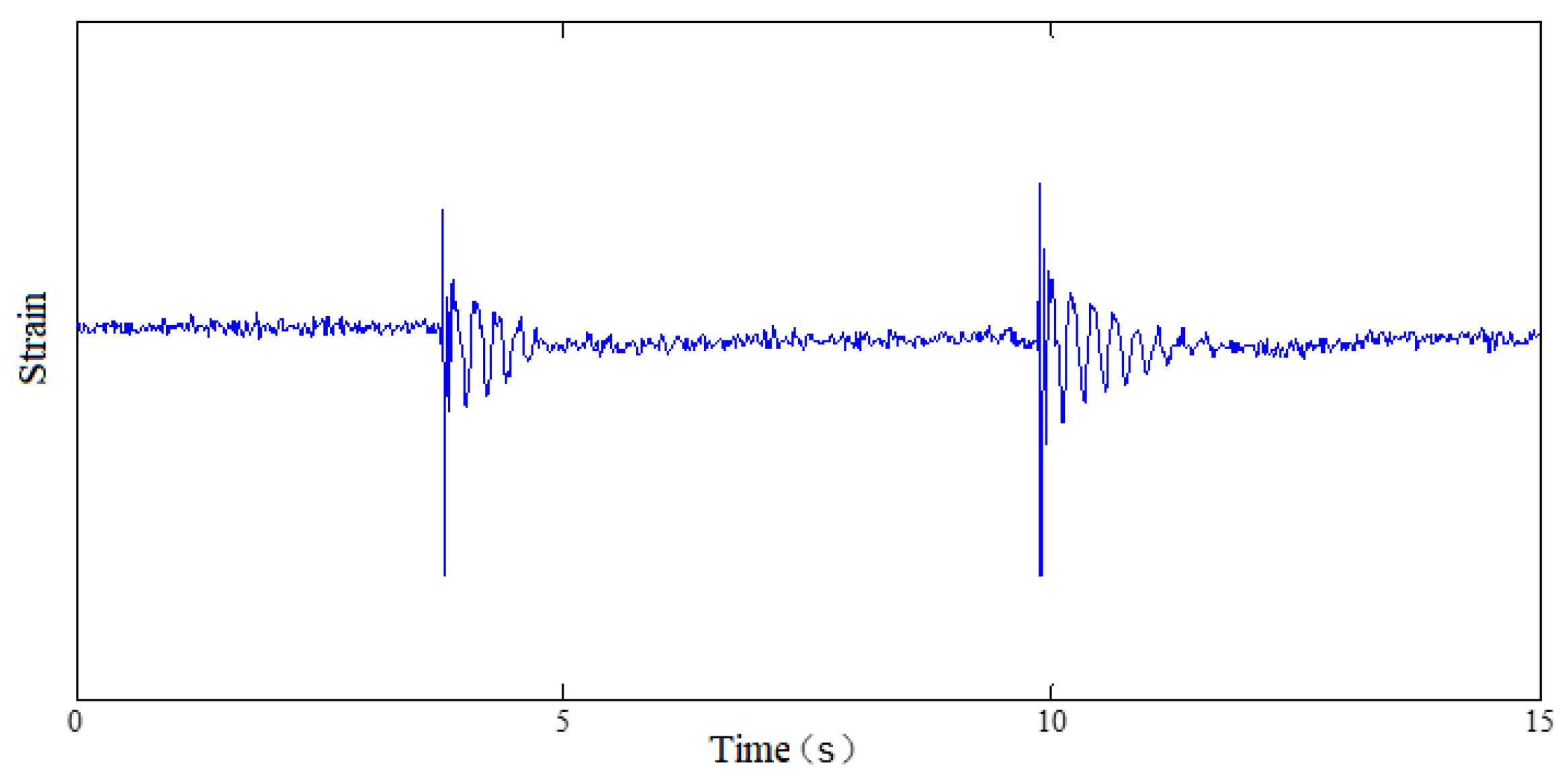
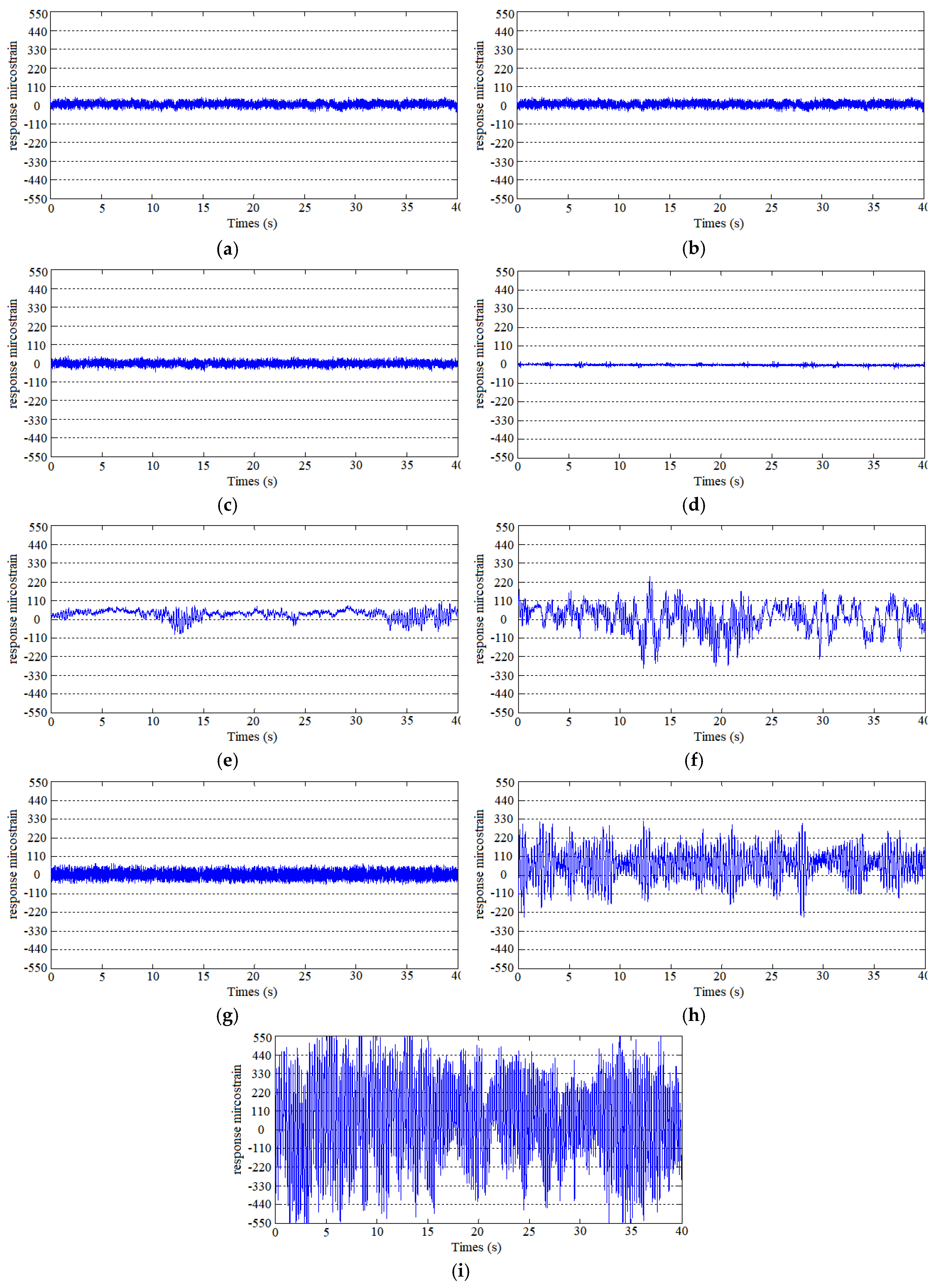
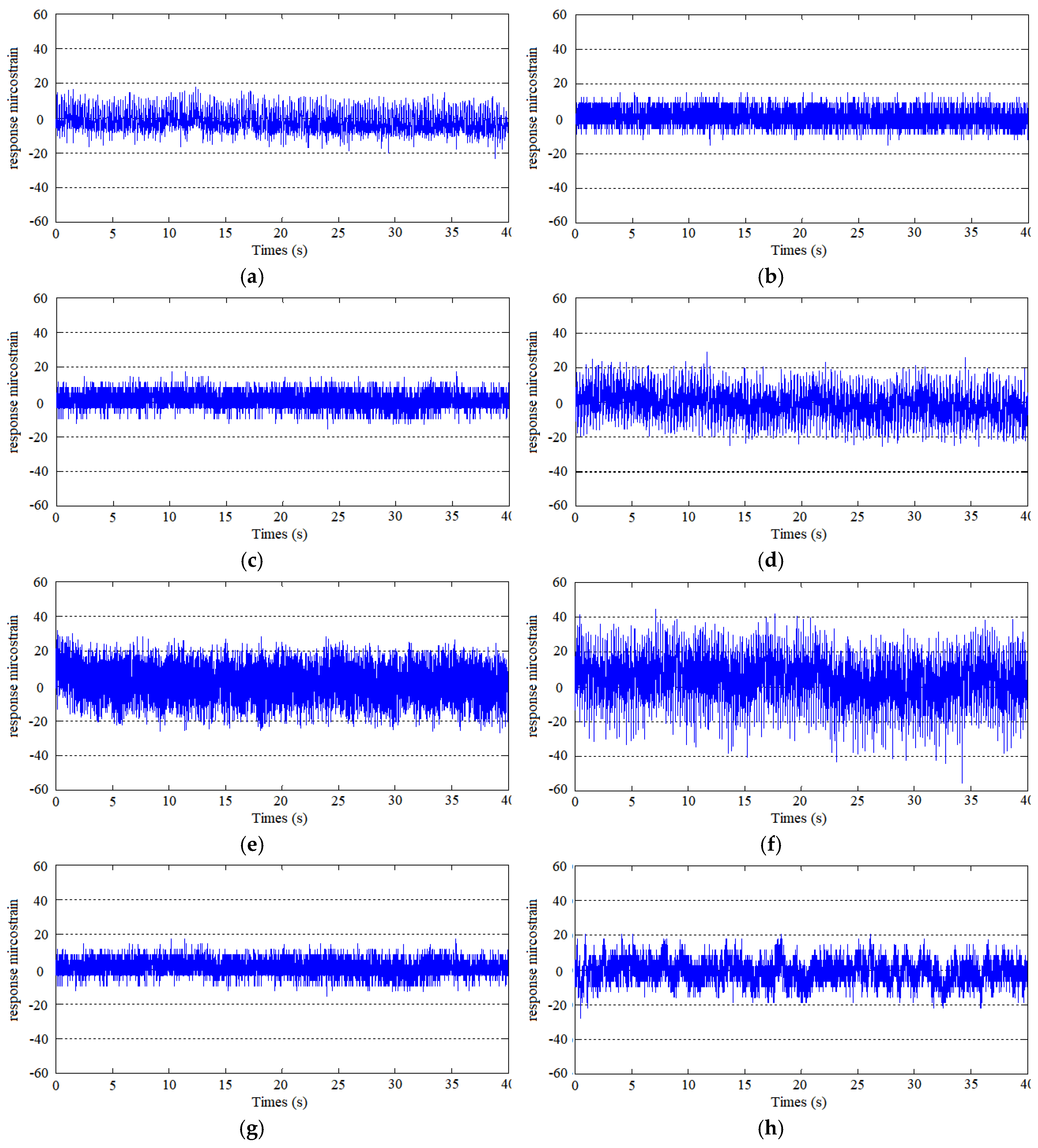
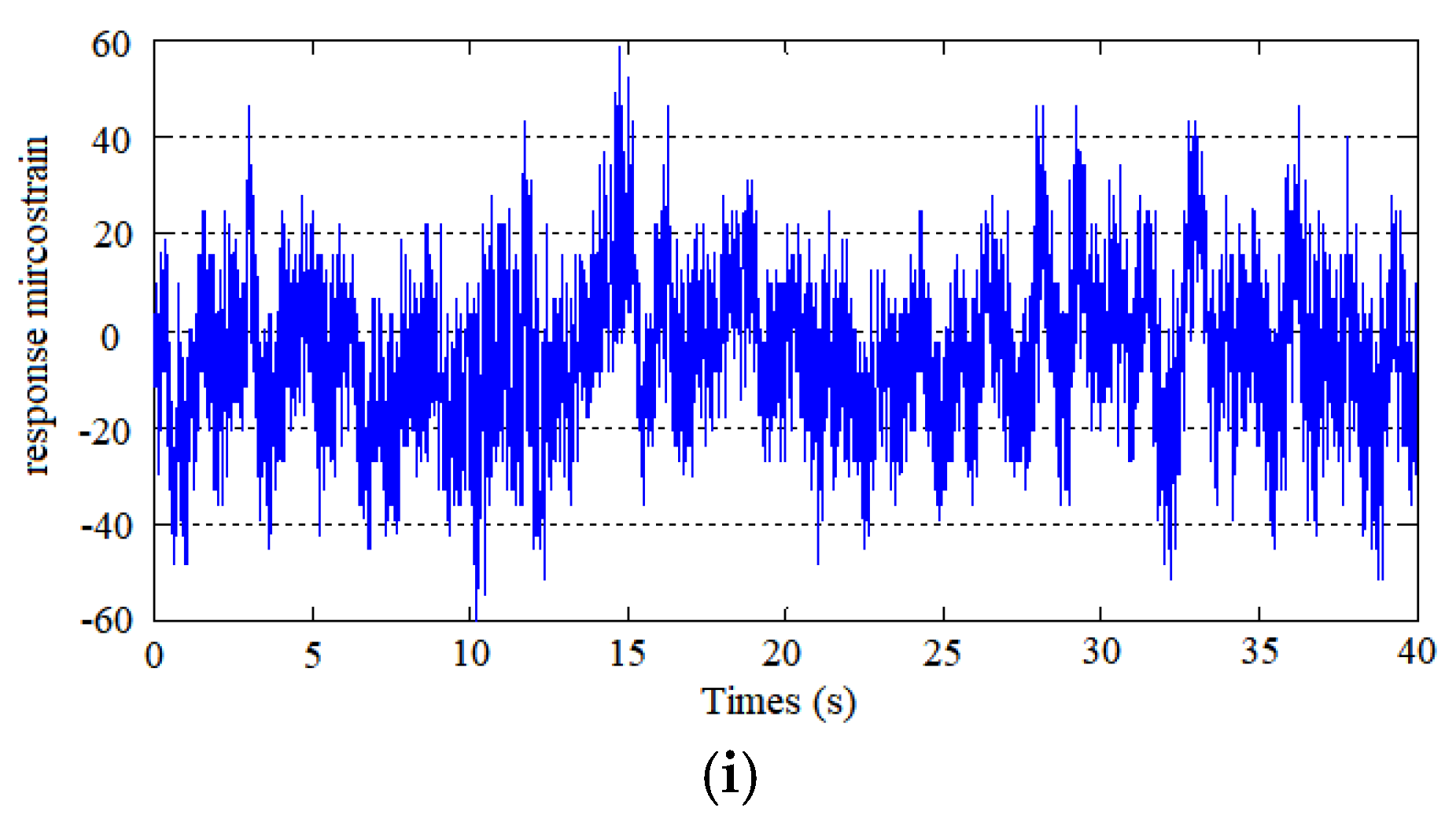
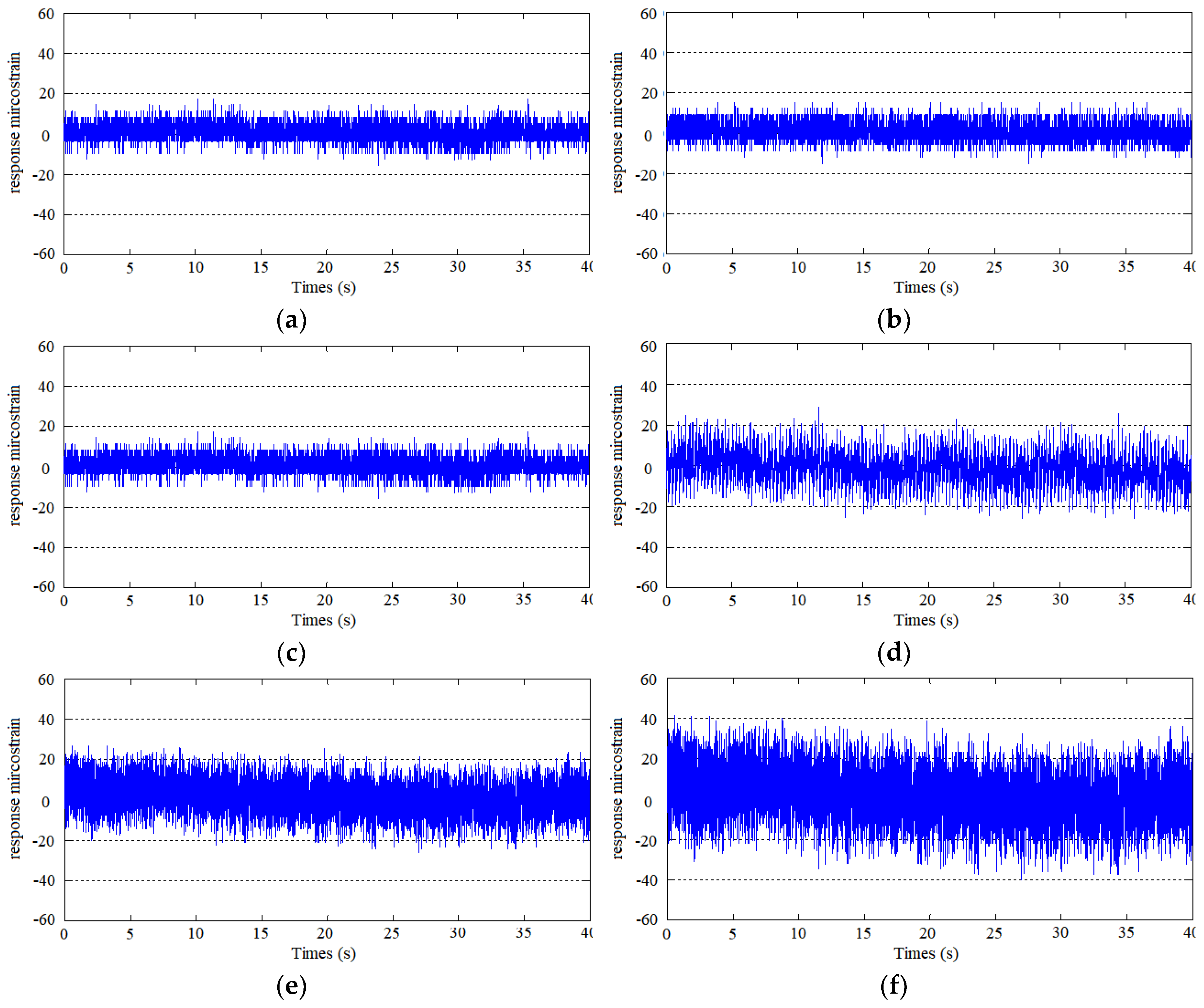
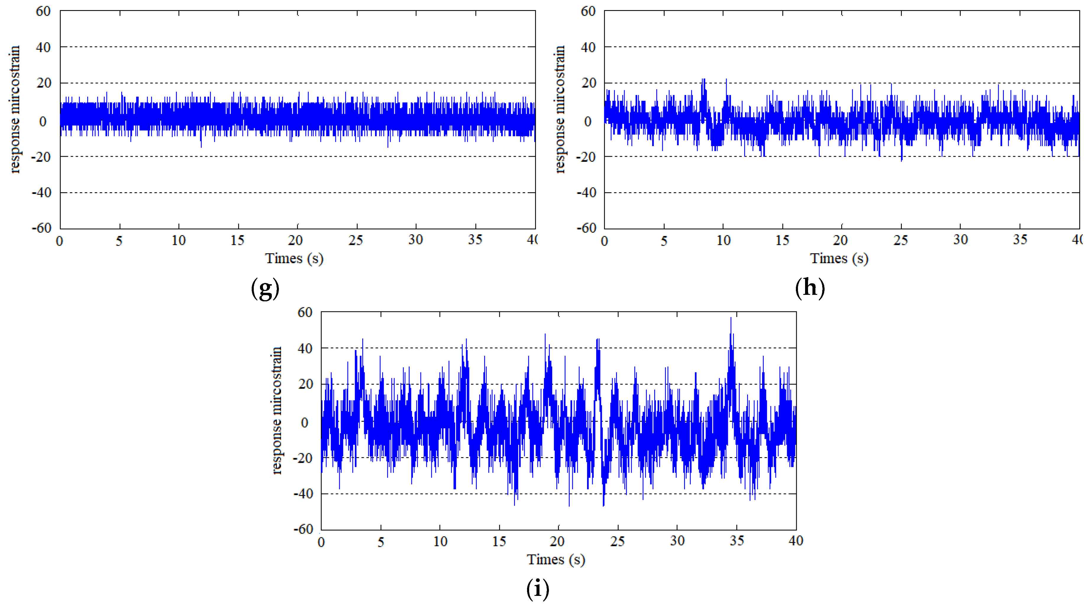
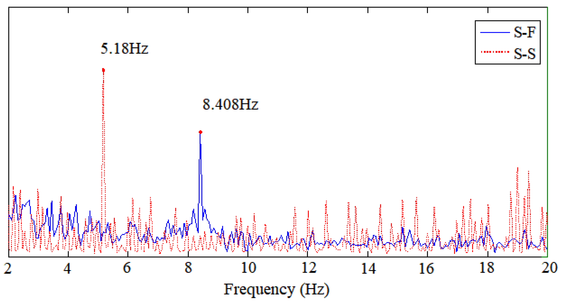
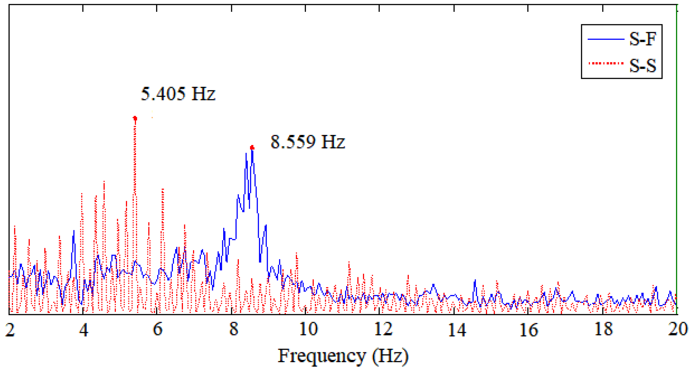
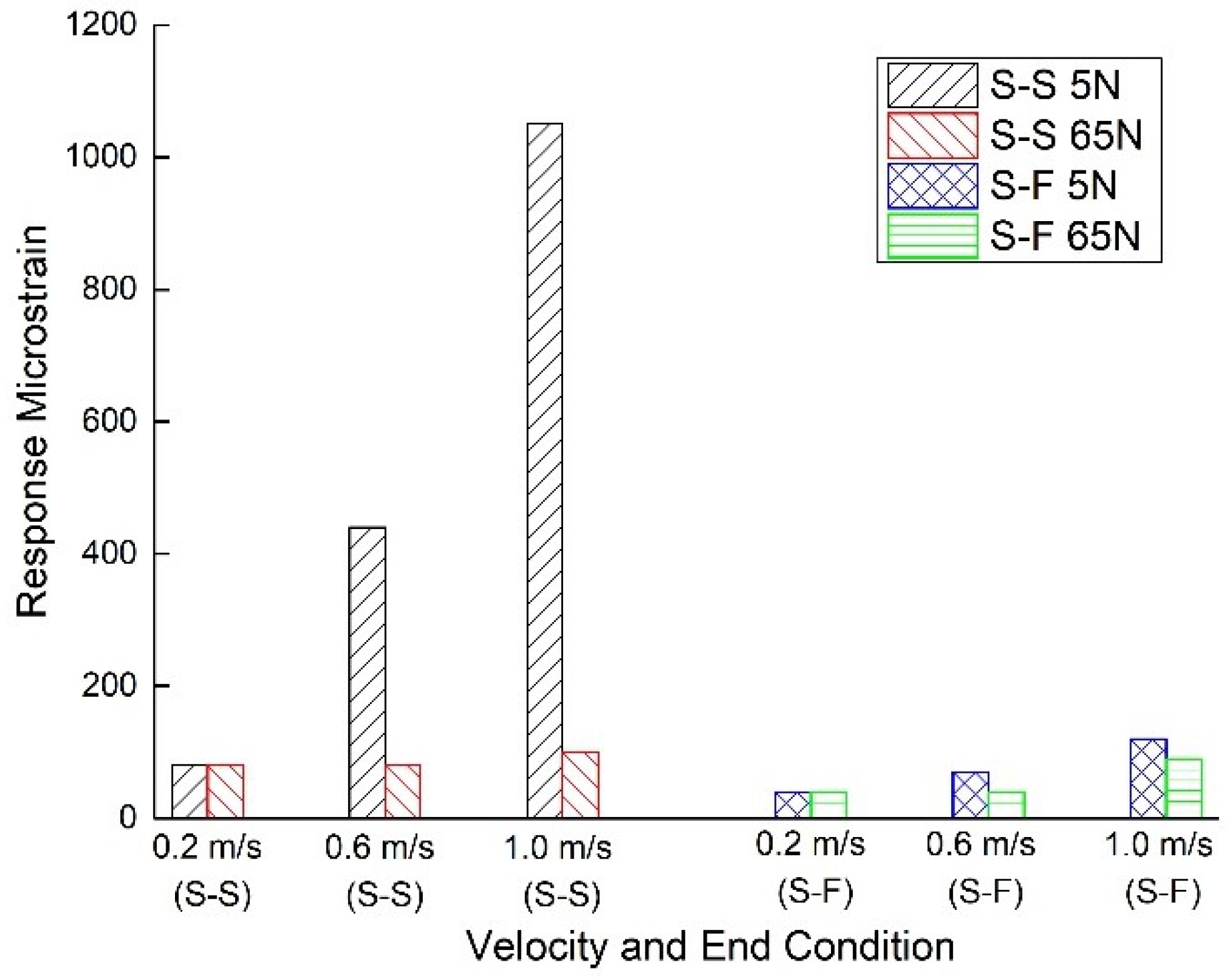
3.2. Vortex-Induced Vibration of the Risers

Generally speaking, the VIV responses of the riser in the flow direction and the cross-flow direction (90° with respect to the flow direction) are obviously different. In flow direction, the displacement is maintained at a relatively stable value, and vibrates slightly after the initial growth [35]. On the other hand, the vibration in the cross-flow direction of the riser is much more significant for the VIV study. It is noted that the cross-flow direction of the riser includes the separation and initiation of the wake and the shedding of vortices, and this fact significantly influences the initiation of the lock-in phenomenon. Moreover, the amplitude of vibration in the middle part of a riser is comparably lager than that at other locations. Therefore, the microstrain curves obtained from the strain gauges in the cross-flow direction (strain gauges ‘c’) at z = 0.5 m are utilized as a typical example presented in this paper.

Figure 4 shows the response microstrain curve of the three risers at z = 0.5 m with a 5 N top tension force and the S-S end condition for flow velocities of 0.2 m/s 0.6 m/s and 1.0 m/s (experiment cases 1–3, 13–15, 25–27).

Figure 4a–c shows that the response strain of the Al riser is not obvious for all velocities. From Figure 4e–f, the response strain curve of the PMMA riser increases with increasing flow velocity; more specifically, 20 με for 0.2 m/s, 150 με for 0.6 m/s, and 330 με for 1.0 m/s. Similarly, the response strain curve of the UPVC riser increases with increasing flow velocity; more specifically, 80 με for 0.2 m/s, 440 με for 0.6 m/s, and 1050 με for 1.0 m/s, from Figure 4g–i.

Figure 5 shows the response microstrain curves of the three risers at z = 0.5 m with a 65 N top tension force and the S-S end condition for flow velocities of 0.2 m/s 0.6 m/s and 1.0 m/s (experiment cases 7–9, 19–21, 31–33).

Comparing Figure 4 and Figure 5, when the top tension force rises to 65 N from 5 N, the response strains of all three risers are not obvious, and the flow velocities have minor effects on them.

Figure 6 shows the response microstrain curves of the three risers at z = 0.5 m with a 5 N top tension force and the S–F end condition for flow velocities of 0.2 m/s 0.6 m/s and 1.0 m/s (experiment cases 4–6, 16–18, 28–30).

From the test results, it is found that the amplitude of the response strain of the risers with the S-F end condition decrease to 1/10 of that of the risers with the S-S end condition. Figure 6a–c shows that the response strain of the Al riser is not obvious for all velocities. From Figure 6e–f, the response strain curve of the PMMA riser increases with increasing flow velocity; more specifically, 40 με for 0.2 m/s and 0.6 m/s and 70 με for 1.0 m/s. Similarly, the response strain curve of the UPVC riser increases with increasing flow velocity; from 30 με to around 120 με.

Figure 7 shows the response microstrain curves of the three risers at z = 0.5 m with a 65 N top tension force and the S-F end condition for flow velocities of 0.2 m/s 0.6 m/s and 1.0 m/s (experiment cases 10–12, 22–24, 34–36).

Figure 7a–c shows that the response strain of the Al riser is not obvious for all velocities. From Figure 7e–f, the amplitudes of response strain for the PMMA riser are similar (40 με) at velocities of 0.2 m/s and 0.6 m/s, and increase to 70 με at velocities of 1.0 m/s. Similarly, the response strain curve of the UPVC riser increases with increasing flow velocity (Figure 7g–i); from about 40 με (0.2 m/s and 0.6 m/s) to around 90 με (1.0 m/s).

From Figure 4, Figure 5, Figure 6 and Figure 7, the VIV of Al risers is not obvious for all conditions, which indicates the significant effect of the modulus. It is also found that the amplitude of VIV with the S-F end condition is much smaller than that of VIV with the S-S end condition when the other parameters are the same. Generally speaking, the amplitude of VIV increases with increasing flow velocity, and the increment speed is much larger for risers with the S-S end condition.

From the figures of the response microstrain of risers, it is obvious that the lock-in phenomenon does not happen for Al risers under all experiment cases. For the PMMA riser, the lock-in phenomenon occurs when the flow velocity reaches 0.6–1.0 m/s with the S-S/S-F end condition and 5 N top tension force. In terms of the UPVC riser, the beginning velocities that lead to the lock-in phenomenon are 0.6 m/s, 0.6–1.0 m/s and 1.0 m/s for 5 N with the S-S end condition, 5 N with S-F end condition, and 65 N with the S-F end condition, respectively.

In addition, the possibility of a riser’s “lock-in” could be evaluated by reduced velocity U_r. Generally speaking, when U_r ranges from 4 to 8 [42], “lock-in” occurs. U_r can be calculated by ${\mathrm{U}}_{\mathrm{r}}=\frac{\mathrm{U}}{{\mathrm{f}}_{\mathrm{n}}\mathrm{D}}$, where U is the flow velocity, f_n is the natural frequency of the riser and D is the outside diameter of the riser. It is found that for experiment cases 14, 15, 18, 21, 24, 26, 29, 32, 35 and 36, the U_r are between 4 and 8. More specifically, the U_r are 4.8, 8.0, 6.2, 6.6, 5.3, 6.8, 5.0, 5.4, 4.6 and 7.7, respectively. Compared to the analysis using the microstrain amplitude of the risers directly, the conclusion gained from the U_r calculation (on the basis of the interrelationship between flow velocity and the natural frequency of the riser) is similar.

We use the UPVC riser as an example, since the its vibration is the most significant in the test. As can be seen in Figure 4, Figure 5, Figure 6 and Figure 7, a flow velocity of 0.2 m/s would not lead to distinct vibration for all the risers, and the frequencies of VIV for the UPVC riser with a 5 N top tension force obtained using power spectral density (PSD) at the flow velocities of 0.6 m/s and 1.0 m/s are shown in Figure 8 and Figure 9.

From Figure 8 and Figure 9, the frequencies of VIV for the UPVC riser with 5 N top tension force and S-S end condition are 5.18 Hz and 5.405 Hz for velocities of 0.6 m/s and 1.0 m/s, respectively, while the frequencies of the UPVC riser with 5 N top tension force and S-F end condition are 8.408 Hz and 8.559 Hz for velocities of 0.6 m/s and 1.0 m/s, respectively. This shows that the S-F end condition leads to greater frequencies of VIV for the risers.

Strouhal number (S_t) is a dimensionless number that describes oscillating flow mechanisms and can be calculated using ${\mathrm{S}}_{\mathrm{t}}=\frac{{\mathrm{f}}_{\mathrm{s}}\mathrm{D}}{\mathrm{U}}$, where f_s is vortex shedding frequency, D is the outside diameter of the riser and U is the flow velocity. Therefore, for cases 26, 27, 29 and 30, the S_t (s) are 0.17, 0.11, 0.28 and 0.17, respectively. As calculated in Section 2.3, the Re (s) are 11,881, 19,802, 11,881 and 19,802, respectively, for these 4 cases. Based on the relationship between Re and S_t, St should be about 0.2. It is found that the value of 0.2 for S_t is a little different from those calculated using vortex shedding frequency. The reasons for this might be: (1) the effect of different parameters, such as tension force, material property and end condition, is not involved in the Re calculation in Section 2.3; or (2) the experimental precision of the test leading to inaccurate results of vortex shedding frequency.

Figure 10 illustrates the effects of top tension force on the amplitude of the VIV for UPVC riser.

From Figure 10, when the flow velocity is 0.2 m/s, the change of top tension force would not lead to the change of amplitude of VIV for the riser. When the velocity rises to 0.6 m/s, the amplitude of VIV for the riser with 65 N top tension force decreases to 18.2% of that with 5 N top tension force and S-S end condition and 57% of that with 5 N top tension force and S-F end condition. Similarly, for the case of a velocity of 1.0 m/s, the effect of larger top tension force is also significant (9.5% with S-S end condition and 75% with S-F end condition, for those with 5 N).

3.3. Grey Relational Analysis of Multiple Parameters

The parameters considered in this paper that affect the amplitude of the VIV for the risers are modulus, flow velocity, top tension force, constraint number and density. In this paper, grey relational analysis (Equations (1)–(8)) is utilized to determine the grey relational grade of the 5 parameters on the amplitude of VIV for the riser.

$$\begin{array}{c}{X}_0=\left\{X_0\left(1\right),X_0\left(2\right),\dots \dots ,X_0\left(36\right)\right\}\\ X_1=\left\{X_1\left(1\right),X_1\left(2\right),\dots \dots ,X_1\left(36\right)\right\}\\ X_2=\left\{X_2\left(1\right),X_2\left(2\right),\dots \dots ,X_2\left(36\right)\right\}\\ X_3=\left\{X_3\left(1\right),X_3\left(2\right),\dots \dots ,X_3\left(36\right)\right\}\\ X_4=\left\{X_4\left(1\right),X_4\left(2\right),\dots \dots ,X_4\left(36\right)\right\}\\ X_5=\left\{X_5\left(1\right),X_5\left(2\right),\dots \dots ,X_5\left(36\right)\right\}\end{array}$$

(1)

where, X₀ is original (reference) data and X₁ to X₅ are the comparative series. More specifically, X₀ is the amplitude of VIV; X₁ is the modulus of material; X₂ is the flow velocity; X₃ is the top tension force; X₄ is the number of constraints; X₅ is the density of material; and numbers 1–36 in brackets are the experiment case number. More specifically, the values of X₀ are obtained from Figure 4, Figure 5, Figure 6 and Figure 7; the values of X₁ and X₅ are obtained from Table 1; Table 3 gives the values X₂ and X₃; in terms of the constraint number X₄, 5 is for S-S (U_x, U_y, U_z at bottom and U_x, U_y at top of the riser) and 8 is for S-F (U_x, U_y, U_z, θ_x, θ_y, θ_z at bottom and U_x, U_y at top of the riser).

The detailed values for X₀ to X₅ are presented below:

$$\{\begin{array}{c}{X}_0=\{30,30,30,20,20,20,25,25,25,20,20,20,20,150,330,40,40,70,20,20,20,40,40,70,80,440,1050,30,40,120,70,70,90,40,40,90\}\\ X_1=\{70,70,70,70,70,70,70,70,70,70,70,70,3.5,3.5,3.5,3.5,3.5,3.5,3.5,3.5,3.5,3.5,3.5,3.5,2,2,2,2,2,2,2,2,2,2,2,2\}\\ X_2=\{0.2,0.6,1,0.2,0.6,1,0.2,0.6,1,0.2,0.6,1,0.2,0.6,1,0.2,0.6,1,0.2,0.6,1,0.2,0.6,1,0.2,0.6,1,0.2,0.6,1,0.2,0.6,1\}\\ X_3=\{5,5,5,5,5,5,65,65,65,65,65,65,5,5,5,5,5,5,65,65,65,65,65,65,5,5,5,5,5,5,65,65,65,65,65,65\}\\ X_4=\{5,5,5,8,8,8,5,5,5,8,8,8,5,5,5,8,8,8,5,5,5,8,8,8,5,5,5,8,8,8,5,5,5,8,8,8\}\\ X_5=\left\{\begin{array}{c}3043,3043,3043,3043,3043,3043,3043,3043,3043,3043,3043,3043,1550,1550,1550,1550,1550,1550\\ 1550,1550,1550,1550,1550,1550,1154,1154,1154,1154,1154,1154,1154,1154,1154,1154,1154,1154\end{array}\right\}\end{array}$$

Here we have to note that, for X₀ to X₅, their measurement units are different, and their values have a very large range, which might cause inaccurate results in the analysis. Therefore, these sequences are normalized to comparability sequences using a process called grey relational generation in GRA. More specifically, the data from Equation (1) is normalized using $Y_i=\raisebox{1ex}{$X_i\left(n\right)$}\!\left/ \!\raisebox{-1ex}{$\overline{{{\displaystyle \sum }}_{n=1}^{36}{X}_i\left(n\right)}$}\right.$ to obtain Equation (2). Where, $\overline{{\displaystyle \sum }_{n=1}^{36}{X}_i\left(n\right)}$ is the mean value of X_i(n), n $\in$ (1,36).

$$\{\begin{array}{c}{Y}_0=\left\{Y_0\left(1\right),Y_0\left(2\right),\dots \dots ,Y_0\left(36\right)\right\}=\left\{\frac{X_0\left(1\right)}{\overline{{{\displaystyle \sum }}_{n=1}^{36}{X}_0\left(n\right)}},\frac{X_0\left(2\right)}{\overline{{{\displaystyle \sum }}_{n=1}^{36}{X}_0\left(n\right)}},\dots \dots ,\frac{X_0\left(36\right)}{\overline{{{\displaystyle \sum }}_{n=1}^{36}{X}_0\left(n\right)}}\right\}\\ Y_1=\left\{Y_1\left(1\right),Y_1\left(2\right),\dots \dots ,Y_1\left(36\right)\right\}=\left\{\frac{X_1\left(1\right)}{\overline{{{\displaystyle \sum }}_{n=1}^{36}{X}_1\left(n\right)}},\frac{X_1\left(2\right)}{\overline{{{\displaystyle \sum }}_{n=1}^{36}{X}_1\left(n\right)}},\dots \dots ,\frac{X_1\left(36\right)}{\overline{{{\displaystyle \sum }}_{n=1}^{36}{X}_1\left(n\right)}}\right\}\\ Y_2=\left\{Y_2\left(1\right),Y_2\left(2\right),\dots \dots ,Y_2\left(36\right)\right\}=\left\{\frac{X_2\left(1\right)}{\overline{{{\displaystyle \sum }}_{n=1}^{36}{X}_2\left(n\right)}},\frac{X_2\left(2\right)}{\overline{{{\displaystyle \sum }}_{n=1}^{36}{X}_2\left(n\right)}},\dots \dots ,\frac{X_2\left(36\right)}{\overline{{{\displaystyle \sum }}_{n=1}^{36}{X}_2\left(n\right)}}\right\}\\ Y_3=\left\{Y_3\left(1\right),Y_3\left(2\right),\dots \dots ,Y_3\left(36\right)\right\}=\left\{\frac{X_3\left(1\right)}{\overline{{{\displaystyle \sum }}_{n=1}^{36}{X}_3\left(n\right)}},\frac{X_3\left(2\right)}{\overline{{{\displaystyle \sum }}_{n=1}^{36}{X}_3\left(n\right)}},\dots \dots ,\frac{X_3\left(36\right)}{\overline{{{\displaystyle \sum }}_{n=1}^{36}{X}_3\left(n\right)}}\right\}\\ Y_4=\left\{Y_4\left(1\right),Y_4\left(2\right),\dots \dots ,Y_4\left(36\right)\right\}=\left\{\frac{X_4\left(1\right)}{\overline{{{\displaystyle \sum }}_{n=1}^{36}{X}_4\left(n\right)}},\frac{X_4\left(2\right)}{\overline{{{\displaystyle \sum }}_{n=1}^{36}{X}_4\left(n\right)}},\dots \dots ,\frac{X_4\left(36\right)}{\overline{{{\displaystyle \sum }}_{n=1}^{36}{X}_4\left(n\right)}}\right\}\\ Y_5=\left\{Y_5\left(1\right),Y_5\left(2\right),\dots \dots ,Y_5\left(36\right)\right\}=\left\{\frac{X_5\left(1\right)}{\overline{{{\displaystyle \sum }}_{n=1}^{36}{X}_5\left(n\right)}},\frac{X_5\left(2\right)}{\overline{{{\displaystyle \sum }}_{n=1}^{36}{X}_5\left(n\right)}},\dots \dots ,\frac{X_5\left(36\right)}{\overline{{{\displaystyle \sum }}_{n=1}^{36}{X}_5\left(n\right)}}\right\}\end{array}$$

(2)

From Equation (2), the detailed results for Y₀ to Y₅ are:

$$\begin{array}{c}{Y}_0=\left\{0.3,0.3,0.3,0.2,0.2,0.2,0.3,0.3,0.3,0.2,0.2,0.2,0.2,1.6,3.6,0.4,0.4,0.8,0.2,0.2,0.2,0.4,0.4,0.8,0.9,4.8,11.4,0.3,0.4,1.3,0.8,0.8,1.0,0.4,0.4,1.0\right\}\\ Y_1=\left\{0.3,0.3,0.3,0.2,0.2,0.2,0.3,0.3,0.3,0.2,0.2,0.2,0.2,1.6,3.6,0.4,0.4,0.8,0.2,0.2,0.2,0.4,0.4,0.8,0.9,4.8,11.4,0.3,0.4,1.3,0.8,0.8,1.0,0.4,0.4,1.0\right\}\\ Y_2=\left\{0.3,1.0,1.7,0.3,1.0,1.7,0.3,1.0,1.7,0.3,1.0,1.7,0.3,1.0,1.7,0.3,1.0,1.7,0.3,1.0,1.7,0.3,1.0,1.7,0.3,1.0,1.7,0.3,1.0,1.7,0.3,1.0,1.7,0.3,1.0,1.7\right\}\\ Y_3=\left\{0.1,0.1,0.1,0.1,0.1,0.1,1.9,1.9,1.9,1.9,1.9,1.9,0.1,0.1,0.1,0.1,0.1,0.1,1.9,1.9,1.9,1.9,1.9,1.9,0.1,0.1,0.1,0.1,0.1,0.1,1.9,1.9,1.9,1.9,1.9,1.9\right\}\\ Y_4=\left\{0.8,0.8,0.8,1.2,1.2,1.2,0.8,0.8,0.8,1.2,1.2,1.2,0.8,0.8,0.8,1.2,1.2,1.2,0.8,0.8,0.8,1.2,1.2,1.2,0.8,0.8,0.8,1.2,1.2,1.2,0.8,0.8,0.8,1.2,1.2,1.2\right\}\\ Y_5=\left\{1.6,1.6,1.6,1.6,1.6,1.6,1.6,1.6,1.6,1.6,1.6,1.6,0.8,0.8,0.8,0.8,0.8,0.8,0.8,0.8,0.8,0.8,0.8,0.8,0.6,0.6,0.6,0.6,0.6,0.6,0.6,0.6,0.6,0.6,0.6,0.6\right\}\end{array}$$

We use ${\Delta }_{0i}=\left|Y_i\left(n\right)-Y_0\left(n\right)\right|$ to obtain the absolute difference of the original data and the comparative series to form Equation (3).

$$\{\begin{array}{c}{\Delta }_{01}=\left\{\left|Y_1\left(1\right)-Y_0\left(1\right)\right|,\left|Y_1\left(2\right)-Y_0\left(2\right)\right|,\dots \dots ,\left|Y_1\left(36\right)-Y_0\left(36\right)\right|\right\}\\ {\Delta }_{02}=\left\{\left|Y_2\left(1\right)-Y_0\left(1\right)\right|,\left|Y_2\left(2\right)-Y_0\left(2\right)\right|,\dots \dots ,\left|Y_2\left(36\right)-Y_0\left(36\right)\right|\right\}\\ {\Delta }_{03}=\left\{\left|Y_3\left(1\right)-Y_0\left(1\right)\right|,\left|Y_3\left(2\right)-Y_0\left(2\right)\right|,\dots \dots ,\left|Y_3\left(36\right)-Y_0\left(36\right)\right|\right\}\\ {\Delta }_{04}=\left\{\left|Y_4\left(1\right)-Y_0\left(1\right)\right|,\left|Y_4\left(2\right)-Y_4\left(2\right)\right|,\dots \dots ,\left|Y_4\left(36\right)-Y_0\left(36\right)\right|\right\}\\ {\Delta }_{05}=\left\{\left|Y_5\left(1\right)-Y_0\left(1\right)\right|,\left|Y_5\left(2\right)-Y_0\left(2\right)\right|,\dots \dots ,\left|Y_5\left(36\right)-Y_0\left(36\right)\right|\right\}\end{array}$$

(3)

From Equation (3), the detailed results for Δ₁ to Δ ₅ are:

$$\{\begin{array}{c}{\Delta }_{01}=\left\{2.5,2.5,2.5,2.6,2.6,2.6,2.5,2.5,2.5,2.6,2.6,2.6,0.1,1.5,3.5,0.3,0.3,0.6,0.1,0.1,0.1,0.3,0.3,0.6,0.8,4.7,11.4,0.2,0.4,1.2,0.7,0.7,0.9,0.4,0.4,0.9\right\}\\ {\Delta }_{02}=\left\{0.0,0.7,1.3,0.1,0.8,1.4,0.1,0.7,1.4,0.1,0.8,1.4,0.1,0.6,1.9,0.1,0.6,0.9,0.1,0.8,1.4,0.1,0.6,0.9,0.5,3.8,9.8,0.0,0.6,0.4,0.4,0.2,0.7,0.1,0.6,0.7\right\}\\ {\Delta }_{03}=\left\{0.2,0.2,0.2,0.1,0.1,0.1,1.6,1.6,1.6,1.6,1.6,1.6,0.1,1.5,3.5,0.3,0.3,0.6,1.6,1.6,1.6,1.4,1.4,1.1,0.7,4.6,11.3,0.2,0.3,1.2,1.1,1.1,0.9,1.4,1.4,0.9\right\}\\ {\Delta }_{04}=\left\{0.4,0.4,0.4,1.0,1.0,1.0,0.5,0.5,0.5,1.0,1.0,1.0,0.6,0.9,2.8,0.8,0.8,0.5,0.6,0.6,0.6,0.8,0.8,0.5,0.1,4.0,10.7,0.9,0.8,0.1,0.0,0.0,0.2,0.8,0.8,0.3\right\}\\ {\Delta }_{05}=\left\{1.3,1.3,1.3,1.4,1.4,1.4,1.3,1.3,1.3,1.4,1.4,1.4,0.6,0.8,2.8,0.4,0.4,0.0,0.6,0.6,0.6,0.4,0.4,0.0,0.3,4.2,10.8,0.3,0.2,0.7,0.2,0.2,0.4,0.2,0.2,0.4\right\}\end{array}$$

Equations (4) and (5) are used to obtain the maximum and minimum value of each data set from Equation (3).

$$\max \Delta =\max \left\{max{\Delta }_{01},max{\Delta }_{02},max{\Delta }_{03},max{\Delta }_{04},max{\Delta }_{05}\right\}=\max \left\{11.36,9.77,11.29,10.67,10.83\right\}=11.36$$

(4)

$$\min \Delta =min\left\{min{\Delta }_{01},min{\Delta }_{02},min{\Delta }_{03},min{\Delta }_{04},min{\Delta }_{05}\right\}=\min \left\{0.08,0.01,0.07,0.01,0.05\right\}=0.01$$

(5)

Equation (6) is utilized to calculate the grey relational coefficient to form Equation (7). Grey relational coefficient is utilized to determine how close each parameter sequence is to its reference sequence; more specifically, the larger the grey relational coefficient, the closer the variable sequence is to its reference sequence.

$$Z_{0i}=\frac{min\Delta +\beta max\Delta }{{\Delta }_{0i}\left(n\right)+\beta max\Delta }$$

(6)

where, $i\in \left[1,5\right],n\in \left[1,36\right]$.

In Equation (6), the identification coefficient $\beta$ is introduced with $\beta \in \left(0, 1\right)$. $\beta$ is utilized to adjust the distinction between normalized reference series and comparative series. According to a previous study, the value of $\beta$ will not change the rank of the grey relational grade and only has an effect on the magnitude of the relational coefficient [43]. In this paper, $\beta =0.5$ is used, as it would lead to medium distinguishing effect and stability [44].

$$\{\begin{array}{c}{Z}_{01}=\left\{Z_{01}\left(1\right),Z_{01}\left(2\right),\dots \dots ,Z_{01}\left(36\right)\right\}=\left\{\frac{min\Delta +\beta max\Delta }{{\Delta }_{01}\left(1\right)+\beta max\Delta },\frac{min\Delta +\beta max\Delta }{{\Delta }_{01}\left(2\right)+\beta max\Delta },\dots \dots ,\frac{min\Delta +\beta max\Delta }{{\Delta }_{01}\left(36\right)+\beta max\Delta }\right\}\\ Z_{02}=\left\{Z_{02}\left(1\right),Z_{02}\left(2\right),\dots \dots ,Z_{02}\left(36\right)\right\}=\left\{\frac{min\Delta +\beta max\Delta }{{\Delta }_{02}\left(1\right)+\beta max\Delta },\frac{min\Delta +\beta max\Delta }{{\Delta }_{02}\left(2\right)+\beta max\Delta },\dots \dots ,\frac{min\Delta +\beta max\Delta }{{\Delta }_{02}\left(36\right)+\beta max\Delta }\right\}\\ Z_{03}=\left\{Z_{03}\left(1\right),Z_{03}\left(2\right),\dots \dots ,Z_{03}\left(36\right)\right\}=\left\{\frac{min\Delta +\beta max\Delta }{{\Delta }_{03}\left(1\right)+\beta max\Delta },\frac{min\Delta +\beta max\Delta }{{\Delta }_{03}\left(2\right)+\beta max\Delta },\dots \dots ,\frac{min\Delta +\beta max\Delta }{{\Delta }_{03}\left(36\right)+\beta max\Delta }\right\}\\ Z_{04}=\left\{Z_{04}\left(1\right),Z_{04}\left(2\right),\dots \dots ,Z_{04}\left(36\right)\right\}=\left\{\frac{min\Delta +\beta max\Delta }{{\Delta }_{04}\left(1\right)+\beta max\Delta },\frac{min\Delta +\beta max\Delta }{{\Delta }_{04}\left(2\right)+\beta max\Delta },\dots \dots ,\frac{min\Delta +\beta max\Delta }{{\Delta }_{04}\left(36\right)+\beta max\Delta }\right\}\\ Z_{05}=\left\{Z_{05}\left(1\right),Z_{05}\left(2\right),\dots \dots ,Z_{05}\left(36\right)\right\}=\left\{\frac{min\Delta +\beta max\Delta }{{\Delta }_{05}\left(1\right)+\beta max\Delta },\frac{min\Delta +\beta max\Delta }{{\Delta }_{05}\left(2\right)+\beta max\Delta },\dots \dots ,\frac{min\Delta +\beta max\Delta }{{\Delta }_{05}\left(36\right)+\beta max\Delta }\right\}\end{array}$$

(7)

From Equation (7), the detailed results for Z₀₁ to Z₀₅ are:

$$\{\begin{array}{c}{Z}_{01}=\left\{0.7,0.7,0.7,0.7,0.7,0.7,0.7,0.7,0.7,0.7,0.7,0.7,1.0,0.8,0.6,1.0,1.0,0.9,1.0,1.0,1.0,1.0,1.0,0.9,0.9,0.5,0.3,1.0,0.9,0.8,0.9,0.9,0.9,0.9,0.9,0.9\right\}\\ Z_{02}=\left\{1.0,0.9,0.8,1.0,0.9,0.8,1.0,0.9,0.8,1.0,0.9,0.8,1.0,0.9,0.7,1.0,0.9,0.9,1.0,0.9,0.8,1.0,0.9,0.9,0.9,0.6,0.4,1.0,0.9,0.9,0.9,1.0,0.9,1.0,0.9,0.9\right\}\\ Z_{03}=\left\{1.0,1.0,1.0,1.0,1.0,1.0,0.8,0.8,0.8,0.8,0.8,0.8,1.0,0.8,0.6,1.0,1.0,0.9,0.8,0.8,0.8,0.8,0.8,0.8,0.9,0.6,0.3,1.0,1.0,0.8,0.8,0.8,0.9,0.8,0.8,0.9\right\}\\ Z_{04}=\left\{0.9,0.9,0.9,0.8,0.8,0.8,0.9,0.9,0.9,0.8,0.8,0.8,0.9,0.9,0.7,0.9,0.9,0.9,0.9,0.9,0.9,0.9,0.9,0.9,1.0,0.6,0.3,0.9,0.9,1.0,1.0,1.0,1.0,0.9,0.9,1.0\right\}\\ Z_{05}=\left\{0.8,0.8,0.8,0.8,0.8,0.8,0.8,0.8,0.8,0.8,0.8,0.8,0.9,0.9,0.7,0.9,0.9,1.0,0.9,0.9,0.9,0.9,0.9,1.0,1.0,0.6,0.3,1.0,1.0,0.9,1.0,1.0,0.9,1.0,1.0,0.9\right\}\end{array}$$

Finally, grey relational grade (GRG) is calculated using Equation (8). GRG is defined as the numerical measure of the relevancy between the reference sequence (X₀) and the comparability sequence (X₁ to X₅), which is between 0 and 1 and represents the level of correlation between the reference sequence and the comparability sequence. The GRG indicates the degree of similarity between the comparability sequence and the reference sequence [45]. More specifically, if a comparability sequence of a parameter gets the highest GRG with the reference sequence, it means that the comparability sequence is most similar to the reference sequence, and the parameter from this comparability sequence has the most significant influence on the reference sequence (VIV amplitude).

$$\{\begin{array}{c}{r}_{01\left(\mathrm{modulus}\right)}=\overline{{\displaystyle \sum }_{n=1}^{36}{Z}_{01}\left(n\right)}=0.8105\\ r_{02\left(\mathrm{velocity}\right)}=\overline{{\displaystyle \sum }_{n=1}^{36}{Z}_{02}\left(n\right)}=0.8838\\ r_{03\left(\mathrm{tension}\right)}=\overline{{\displaystyle \sum }_{n=1}^{36}{Z}_{03}\left(n\right)}=0.8354\\ r_{04\left(\mathrm{constraints}\right)}=\overline{{\displaystyle \sum }_{n=1}^{36}{Z}_{04}\left(n\right)}=0.8756\\ r_{05\left(\mathrm{density}\right)}=\overline{{\displaystyle \sum }_{n=1}^{36}{Z}_{05}\left(n\right)}=0.8643\end{array}$$

(8)

As mentioned above, if a GRG calculated by Equation (8) is higher than others, it means that this particular comparability sequence has a greater effect than others on the reference sequence [45]. In this study, it can be seen that $r_{02\left(\mathrm{velocity}\right)}>r_{04\left(\mathrm{constraints}\right)}>r_{05\left(\mathrm{density}\right)}>r_{03\left(\mathrm{tension}\right)}>r_{01\left(\mathrm{modulus}\right)}$.

As can be seen from the results, these five parameters have a similar effect on the amplitude of VIV for the riser, since their GRG values are close to each other. However, according to the relative magnitudes of GRG for each parameter, the flow velocity has the biggest influence, then the number of constraints, followed by the density of material, followed by the top tension force, and finally the modulus of material.

4. Conclusions

This paper presents the experimental study on vortex-induced vibration of risers with the following parameters: material properties (modulus and density), end condition, top tension force and flow velocity. Based on the variables of each parameter, 36 experiment cases were carried out in total. The natural frequencies of each riser situations, the response microstrain for all experiment cases, and the frequency of VIV for the risers were obtained. According to these results, the effect of each parameter was discussed and the grey relational grade of these parameters on the amplitude of VIV for riser was calculated using grey relational analysis.

It was found in this paper:

(1)

The modulus of the riser, number of constraints and the top tension force is positively correlated with the natural vibration frequency.

(2)

The increase of modulus, number of constraints and top tension force and the reduction of velocity lead to a decrease in the amplitude of VIV for riser.

(3)

The lock-in phenomenon does not happen for Al riser under all experiment cases, while for the PMMA riser and the UPVC riser, the lock-in phenomenon occurs in specific experiment cases.

(4)

The S-F end condition leads to higher frequencies of VIV for the risers.

(5)

The grey relational grade of the influence on the amplitude of VIV for riser are: $r_{02\left(\mathrm{velocity}\right)}>r_{04\left(\mathrm{constraints}\right)}>r_{05\left(\mathrm{density}\right)}>r_{03\left(\mathrm{tension}\right)}>r_{01\left(\mathrm{modulus}\right)}$.

References

1. Wang, C.; Shankar, K.; Morozov, E.V. Tailored local design of deep sea frp composite risers. Adv. Compos. Mater. 2015, 24, 375–397. [Google Scholar] [CrossRef]
2. Wang, C.; Shankar, K.; Morozov, E.V. Global design and analysis of deep sea frp composite risers under combined environmental loads. Adv. Compos. Mater. 2017, 26, 79–98. [Google Scholar] [CrossRef]
3. Chakrabarti, S.K.; Frampton, R.E. Review of riser analysis techniques. Appl. Ocean Res. 1982, 4, 73–90. [Google Scholar] [CrossRef]
4. Sparks, C.P. Lightweight composite production risers for a deep water tension leg platform. In Proceedings of the Fifth International Offshore Mechanics and Arctic Engineering (OMAE) Symposium, Tokyo, Japan, 13–18 April 1986; pp. 86–93. [Google Scholar]
5. Sparks, C.P.; Odru, P.; Bono, H.; Metivaud, G. Mechanical testing of high-performance composite tubes for tlp production risers. In Proceedings of the Offshore Technology Conference, Houston, TX, USA, 2–5 May 1988. [Google Scholar]
6. Salama, M.M.; Johnson, D.B.; Long, J.R. Composite production riser-testing and qualification. SPE Prod. Facil. 1998, 13, 170–177. [Google Scholar] [CrossRef]
7. Smith, K.L.; Leveque, M.E. Ultra-Deepwater Production Systems Technical-Progress Report; ConocoPhillips Company: Houston, TX, USA, 2003. [Google Scholar]
8. Smith, K.L.; Leveque, M.E. Ultra-Deepwater Production Systems-Final Report; ConocoPhillips Company: Houston, TX, USA, 2005. [Google Scholar]
9. Picard, D.; Hudson, W.; Bouquier, L.; Dupupet, G.; Zivanovic, I. Composite carbon thermoplastic tubes for deepwater application. In Proceedings of the Offshore Technology Conference, Houston, TX, USA, 30 April–3 May 2007. [Google Scholar]
10. Wang, C.; Shankar, K.; Ashraf, M.A.; Morozov, E.V.; Ray, T. Surrogate-assisted optimisation design of composite riser. Proc. Inst. Mech. Eng. Part L J. Mater. Des. Appl. 2016, 230, 18–34. [Google Scholar]
11. Smits, A.; Neto, T.B.; Boer, H.D. Thermoplastic composite riser development for ultradeep water. In Proceedings of the Offshore Technology Conference, Houston, TX, USA, 30 April–3 May 2018; p. 13. [Google Scholar]
12. Wang, C.; Shankar, K.; Morozov, E.V. Tailored design of top-tensioned composite risers for deep-water applications using three different approaches. Adv. Mech. Eng. 2017, 9, 1687814016684271. [Google Scholar] [CrossRef]
13. Sarpkaya, T. Fluid forces on oscillating cylinders. J. Waterw. Port Coast. Ocean Div. 1978, 104, 275–290. [Google Scholar]
14. Gopalkrishnan, R. Vortex Induced Forces on Oscillating Bluff Cylinders; Massachusetts Institute of Technology: Cambridge, MA, USA, 1993. [Google Scholar]
15. Khalak, A.; Williamson, C.H.K. Motions, forces and mode transitions in vortex-induced vibrations at low mass-damping. JFS 1999, 13, 813–851. [Google Scholar] [CrossRef]
16. Govardhan, R.; Williamson, C.H.K. Resonance forever: Existence of a critical mass and an infinite regime of resonance in vortex-induced vibration. J. Fluid Mech. 2002, 473, 147–166. [Google Scholar] [CrossRef]
17. Tang, Y.; Qin, Z.; Zhang, J.; Wang, B. Prediction model and influence factors on vortex-induced vibration of deepwater risers. J. Harbin Eng. Univ. 2017, 38, 338–343. [Google Scholar]
18. Tsahalis, D.; Jones, W. The effect of the sea-bottom proximity of the fatigue life of suspended spans of offshore pipelines undergoing vortex-induced vibrations. In Proceedings of the Offshore Technology Conference, Houston, TX, USA, 3–6 May 1982. [Google Scholar]
19. Tsahalis, D.T. Vortex-induced vibrations due to steady and wave-induced currents of a flexible cylinder near a plane boundary. J. Offshore Mech. Arct. Eng. 1987, 109, 112–118. [Google Scholar] [CrossRef]
20. Tsahalis, D. Vortex-induced vibrations of a flexible cylinder near a plane boundary exposed to steady and wave-induced currents. J. Energy Resour. Technol. 1984, 106, 206–213. [Google Scholar] [CrossRef]
21. Tsahalis, D.; Jones, T.W. Vortex-induced vibrations of a flexible cylinder near a plane boundary in steady flow. In Proceedings of the Offshore Technology Conference, Houston, TX, USA, 4–7 May 1981. [Google Scholar]
22. Hartlen, R.T.; Currie, I.G. Lift-oscillator model of vortex-induced vibration. J. Eng. Mech. Div. 1970, 96, 577–591. [Google Scholar]
23. Skop, R.A.; Griffin, O.M. On a theory for the vortex-excited oscillations of flexible cylindrical structures. J. Sound Vib. 1975, 41, 263–274. [Google Scholar] [CrossRef]
24. Kim, W.J.; Perkins, N.C. Two-dimensional vortex-induced vibration of cable suspensions. JFS 2002, 16, 229–245. [Google Scholar] [CrossRef]
25. Facchinetti, M.L.; de Langre, E.; Biolley, F. Coupling of structure and wake oscillators in vortex-induced vibrations. JFS 2004, 19, 123–140. [Google Scholar] [CrossRef]
26. Wu, X.M.; Huang, W.P. A New Model for Predicting Vortex-Induced Vibration of a Long Flexible Riser with Large Deformation. J. Vib. Shock 2013, 32, 21–25. [Google Scholar]
27. Guo, H.Y.; Zhao, W.; Wang, F. Experimental investigation of the effect of internal flow on top tension of the riser. Period. Ocean Univ. China 2015, 45, 102–109. [Google Scholar]
28. Lou, M.; Yu, C. Dynamic responses of a riser under combined excitation of internal waves and background currents. Int. J. Nav. Arch. Ocean Eng. 2014, 6, 685–699. [Google Scholar] [CrossRef]
29. Tang, Y.G.; Shao, W.D.; Zhang, J.; Wang, L.Y.; Gui, L. Dynamic Response Analysis for Coupled Parametric Vibration and Vortex-Induced Vibration of Top-Tensioned riser in Deep-Sea. Eng. Mech. 2013, 30, 282–286. [Google Scholar]
30. Liu, J.; Guo, H.; Zhao, J. Numerical simulaiton of flow around two tandem circular cylinder of equal dimeter. Period. Ocean Univ. China 2013, 43, 92–97. [Google Scholar]
31. Ji, C.; Xiao, Z.; Wang, Y.; Wang, H. Numerical investigation on vortex-induced vibration of an elastically mounted circular cylinder at low reynolds number using the fictitious domain method. IJCFD 2011, 25, 207–221. [Google Scholar] [CrossRef]
32. Tan, L.B.; Chen, Y.; Jaiman, R.K.; Sun, X.; Tan, V.B.C.; Tay, T.E. Coupled fluid–structure simulations for evaluating a performance of full-scale deepwater composite riser. Ocean Eng. 2015, 94, 19–35. [Google Scholar] [CrossRef]
33. Huang, K.Z. Composite ttr design for an ultradeepwater tlp. In Proceedings of the Offshore Technology Conference, Houston, TX, USA, 2–5 May 2005. [Google Scholar]
34. Chen, Y.; Tan, L.B.; Jaiman, R.K.; Sun, X.; Tay, T.E.; Tan, V.B.C. Global-local analysis of a full-scale composite riser during vortex-induced vibration. In Proceedings of the ASME 2013 32nd International Conference on Ocean, Offshore and Arctic Engineering, Nantes, France, 9–14 June 2013; Volume 7. [Google Scholar]
35. Wang, C.; Sun, M.; Shankar, K.; Xing, S.; Zhang, L. Cfd simulation of vortex induced vibration for frp composite riser with different modeling methods. Appl. Sci. 2018, 8, 684. [Google Scholar] [CrossRef]
36. Morán, J.; Granada, E.; Míguez, J.L.; Porteiro, J. Use of grey relational analysis to assess and optimize small biomass boilers. Fuel Process. Technol. 2006, 87, 123–127. [Google Scholar] [CrossRef]
37. Ju-Long, D. Control problems of grey systems. Syst. Control Lett. 1982, 1, 288–294. [Google Scholar] [CrossRef]
38. Deng, J.L. Introduction to grey system theory. J. Grey Syst. 1989, 1, 1–24. [Google Scholar]
39. Yeh, M.F.; Lu, H.C. Evaluating weapon systems based on grey relational analysis and fuzzy arithmetic operations. J. Chin. Inst. Eng. 2000, 23, 211–221. [Google Scholar] [CrossRef]
40. Lu, J.-C.; Yeh, M.-F. Robot path planning based on modified grey relational analysis. CySys 2002, 33, 129–159. [Google Scholar] [CrossRef]
41. Chang, K.; Yeh, M. Grey relational analysis based approach for data clustering. IEE Proc. Vis. Image Signal Process. 2005, 152, 165–172. [Google Scholar] [CrossRef]
42. Blevins, R.D. Flow-Induced Vibratin, 2nd ed.; Krieger Publishing Company: Malabar, FL, USA, 2001. [Google Scholar]
43. Jiang, B.C.; Szu-Lang, T.; Chien-Chih, W. Machine vision-based gray relational theory applied to ic marking inspection. IEEE Trans. Semicond. Manuf. 2002, 15, 531–539. [Google Scholar] [CrossRef]
44. Lin, S.J.; Lu, I.J.; Lewis, C. Grey relation performance correlations among economics, energy use and carbon dioxide emission in taiwan. Energy Policy 2007, 35, 1948–1955. [Google Scholar] [CrossRef]
45. Fung, C.-P. Manufacturing process optimization for wear property of fiber-reinforced polybutylene terephthalate composites with grey relational analysis. Wear 2003, 254, 298–306. [Google Scholar] [CrossRef]
Figure 1. Testing instrumentation. (a) Current generation system; (b) velocity monitoring system; (c) end condition system; (d) data acquisition system.
Applsci 08 02411 g001aApplsci 08 02411 g001b
Figure 2. Riser model used in the experiment. (a) Sketch map of the model riser; (b) risers used in the experiment; (c) holistic test setup for the riser.
Applsci 08 02411 g002
Figure 3. Strain response under beating.
Applsci 08 02411 g003
Figure 4. Response microstrain curves of the three risers at z = 0.5 m with 5 N top tension force and S-S end condition. (a) 0.2 m/s, Al, case 1; (b) 0.6 m/s, Al, case 2; (c) 1.0 m/s, Al, case 3; (d) 0.2 m/s, PMMA, case 13; (e) 0.6 m/s, PMMA, case 14; (f) 1.0 m/s, PMMA, case 15; (g) 0.2 m/s, UPVC, case 25; (h) 0.6 m/s, UPVC, case 26; (i) 1.0 m/s, UPVC, case 33.
Applsci 08 02411 g004
Figure 5. Response microstrain curves of the three risers at z = 0.5 m with 65 N top tension force and S –S end condition. (a) 0.2 m/s, Al, case 7; (b) 0.6 m/s, Al, case 8; (c) 1.0 m/s, Al, case 9; (d) 0.2 m/s, PMMA, case 19; (e) 0.6 m/s, PMMA, case 20; (f) 1.0 m/s, PMMA, case 21; (g) 0.2 m/s, UPVC, case 31; (h) 0.6 m/s, UPVC, case 32; (i) 1.0 m/s, UPVC, case 33.
Applsci 08 02411 g005
Figure 6. Response microstrain curves of the three risers at z = 0.5 m with a 5 N top tension force and the S-F end condition. (a) 0.2 m/s, Al, case 4; (b) 0.6m/s, Al, case 5; (c) 1.0 m/s, Al, case 6; (d) 0.2 m/s, PMMA, case 16; (e) 0.6 m/s, PMMA, case 17; (f) 1.0 m/s, PMMA, case 18; (g) 0.2 m/s, UPVC, case 28; (h) 0.6 m/s, UPVC, case 29; (i) 1.0 m/s, UPVC, case 30.
Applsci 08 02411 g006aApplsci 08 02411 g006b
Figure 7. Response microstrain curves of the three risers at z = 0.5 m with a 65 N top tension force and the S-F end condition. (a) 0.2 m/s, Al, case 10; (b) 0.6m/s, Al, case 11; (c) 1.0 m/s, Al, case 12; (d) 0.2 m/s, PMMA, case 22; (e) 0.6 m/s, PMMA, case 23; (f) 1.0 m/s, PMMA, case 24; (g) 0.2 m/s, UPVC, case 34; (h) 0.6 m/s, UPVC, case 35.
Applsci 08 02411 g007aApplsci 08 02411 g007b
Figure 8. PSD of the UPVC risers with two different end conditions (U = 0.6 m/s).
Applsci 08 02411 g008
Figure 9. PSD of the UPVC risers with two different end conditions (U = 1.0 m/s).
Applsci 08 02411 g009
Figure 10. Effects of top tension force on the amplitude of the VIV for UPVC riser.
Applsci 08 02411 g010