Abstract
High penetration of wind power plants may have an adverse impact on power systems’ stability by reducing the inertia, and problems like frequency stability could appear due to total inertia in the system being reduced, making the power system more vulnerable to disturbances. However, most recent grid codes include an emulation inertia requirement for wind power plants, because modern wind turbines are capable of providing virtual inertia through power electronic converter controls to improve frequency stability issues. Because of this, it is necessary that the inertia estimation analyze and quantify the impact of the inertia reduction in power systems. In this paper, an implementation of a methodology for the inertia estimation of wind power plants is presented. It is evaluated through synchrophasor measurements obtained from a Real-Time Digital Simulator (RTDS) implementation, using industrial Phasor Measurement Units (PMUs). This methodology is based on the swing equation. Furthermore, a comparison of the results obtained between two professional tools RSCAD and DIgSILENT PowerFactory is performed, in order to evaluate the accuracy and the robustness of the methodology. This methodology is applied for the inertia estimation of an equivalent of the southeast zone of the Mexican power system, where there is a large-scale penetration of wind power plants. The results demonstrate that this methodology can be applied in real power systems using PMUs.
1. Introduction
The amount of wind power generation has grown in recent years, providing 3% of global power, for example, China is leading with 164 GW, the United States with 6 GW, Germany with 6 GW, India with 4 GW, and the U.K. with 4 GW [1]. This is along with the aim of reducing the dependence on fossil fuels and mitigating the adverse effects of global warming [2,3]. Wind generation brings benefits [4,5], but also challenges for power systems [6,7], especially when there is a high penetration of wind power plants. Therefore, it is essential to conduct studies about the stability and operation of power systems, including this type of plant.
The determination of the stability of the power system is important; it lets us know if the power system is able to regain a state of equilibrium after the system is subjected to a physical disturbance [8]. Inertia is the parameter that represents the capability of rotating machines to store and inject their kinetic energy in the system. The level of inertia influences the Rate Of Change of Frequency (ROCOF) and transient frequency values during a system perturbation. The transient value of the system frequency is important because variations in the frequency caused by an inertia decrease can raise the risk of reaching values that are dangerous for the system frequency stability (generator trip, load shedding intervention, etc.) [9].
On the other hand, wind turbine generators are decoupled from the grid by power electronic converters; thus, they do not directly contribute to system inertia [10], and large-scale penetration of non-inertial wind generators in the power system will result in reduced system inertia [11,12,13]. This reduction has a substantial impact on frequency regulation [14]. Therefore, the inertia estimation can be used as an input for the control of power electronic converters and energy storage systems, among others, helping to maintain the system frequency stability during disturbances.
In the literature, potential applications have been proposed for the results obtained from the inertia estimation. For instance, in [15], the inertia estimation was used to enhance the dynamic operation and performance of a power grid against frequency stability problems, while in [16], an inertia estimation algorithm was used in combination with the ROCOF and a derivative control of a High Voltage Direct Current (HVDC) controller to provide active power and enhance the inertia response of conventional generators when the power demand changes. However, the main application of the inertia estimation in wind power plants is to set the references of the synthetic inertial controllers included in these plants [17,18]; these controllers are based on the concept of hidden inertia emulation of wind power plants, which increases the electric power output during the initial stages of stability frequency issues using the kinetic energy from moving parts. The concept of synthetic inertia provides a boost energy in a similar way as a synchronous generator with real inertia and reduces stability frequency issues.
This paper improves and evaluates the methodology presented in [11] for the estimation of the inertia available in hydro and wind power plants based on the measurements obtained from PMUs. The methodology was modified using a fourth-order finite-difference approximation to calculate the second-order derivative of the swing equation, and the results obtained are way better. Besides, the methodology is tested using measurements obtained from industrial PMUs in a test power system implemented in an RTDS, to test its practical application, and not only using offline simulations, as reported previously. In addition, the methodology is applied to an equivalent of the Mexican southeast power system, where there is high penetration of wind and hydropower generation.
In order to evaluate the accuracy and robustness of the inertia estimation, a power system was implemented as an experimental setup in a Real-Time Digital Simulator (RTDS), and the results of the inertia estimation were compared against the professional software DIgSILENT PowerFactory [19].
The rest of the paper is organized as follows: in Section 2 is presented the literature review referent to the inertia estimation in power systems; in Section 3, the methodology to estimate the inertia constant of the generation units is presented; Section 4 shows the inertia estimation of the experimental validation; Section 5 presents the behavior of the inertia estimation when the generated active power is varied; Section 6 presents the results obtained with the application of the methodology in the southeast zone of the Mexican electric system; finally, Section 7 draws the main conclusions of this paper.
2. Methods for Inertia Estimation
To address frequency stability issues, some works have been proposed to estimate the inertia in power systems with the purpose to improve the frequency stability and enable higher penetration of wind power plants [14,20].
In [20], a virtual inertia was estimated by using the frequency deviation measurements in a microgrid. The method was based on the swing equation, and the value of the inertia was used for tuning load frequency controllers of the generation units and calculating the active power required for an energy system storage, composed by Ultracapacitors (UC), to improve the frequency stability problems.
The work in [21] calculated a synthetic inertia by means of a transfer function that represented the electromechanical behavior of a synchronous generator. The inertia estimation was done considering load changes and frequency deviations read of the power system.
In the work reported in [22], a virtual inertia was estimated through the swing equation of synchronous machines. The system was linearized with respect to the speed of the generator, and the inertia was determined by the balance between the mechanical and active power of the generation units.
The work in [23] estimated the power system inertia through a simulation model and frequency measurements from PMUs. In the inertia estimation, the frequency and the total active power at the connection point just after the disturbance were considered.
In [24], the inertia estimation was based on an approximation of the total power change after a disturbance has occurred. This methodology used the average frequency of the system and the first instant after the application of the disturbance to estimate the inertia.
The aforementioned methodologies were based on the swing equation and transients events, like the ROCOF, and some of them used off-line measurements, such as the power system frequency, which led to a low inertia estimation accuracy [25]. On the other hand, the method presented in [24] provided low inertia estimation error by employing particle swarm optimization, but the accuracy of this method depended on the load power change model and a large number of parameters such as currents, load impedance, power change measurements after the disturbance, and the frequency average of the system.
Table 1 shows the differences between the main methodologies proposed in the literature for the inertia estimation and the methodology used in this research. The plus and minus signs indicate if the methodology contains (+) or not (−) the characteristic evaluated in Table 1, respectively. The principal characteristics used in the comparison are the simplicity of the algorithm, online implementation, accuracy of the inertia estimation on the first oscillation, mean error, a smaller number of parameters used for the estimation, and the robustness of the algorithm against variations in the system.

Table 1.
Comparison among methodologies for the inertia estimation.
In contrast with the the mentioned methods, the methodology used in this paper only needs the bus angle deviation at generation buses obtained from PMUs and real power measurements. It has a considerable balance of accuracy on the first oscillation, a simplified algorithm, robustness in the presence of variations in the system, and low error in the estimation of the inertia in the generation units. However, a disadvantage of this methodology is that the accuracy is reduced when the system is subject to small perturbations such as load variations. The methodology uses the time when the perturbation starts to determinate the peak value of the first angular oscillation. In its current form, this methodology does not include any technique for the detection of perturbations.
3. Methodology for the Inertia Estimation
Typically, the natural inertia of synchronous generator units responds voluntarily when the system is subject to disturbances, without any control actions [26,27]. This behavior can be achieved in wind power plants through power electronic converters by wind turbine inertia controls, even when they are decoupled partially or completely from the grid [12,28,29]. This assumption is valid because modern wind turbine controllers can convert the kinetic energy into active power, i.e., control functions achieved by power converter controls can be seen as the virtual inertia of wind generators [14,18]. This is shown in Figure 1. Through both natural and virtual inertias, active power is released to the power system from the kinetic energy of generation units. In the case of wind power plants, this is done through power electronics converters and wind turbine controls that extract the kinetic energy from moving parts and convert it into real power output [17,18]. This characteristic of inertia response in wind power plants can be described in a format similar to conventional generator units by the swing equation, which is directly derived from Newton’s law of motion on rotating objects. Due to this correlation between the virtual inertia of wind power plants and the real inertia of synchronous generation units, an inertia can be estimated for wind power plants in a format similar to conventional generators [11].
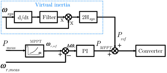
Figure 1.
Virtual inertia concept in wind power plants.
The characteristic inertia response can be represented by the swing equation, which describes the change between the axis of the rotor and the magnetic field. This change is produced when a disturbance occurs in the power system. As a result, the rotor accelerates or decelerates with respect to system synchronous speed [26]. The swing equation is given by the next expression [27,30]:
where is the rated speed of the system, is the rotor angle, is the mechanical power, is the electrical power, is the damping factor, and is the derivative of the rotor angle.
Equation (1) represents the dynamic response of the inertia of the synchronous machines or a group of synchronous machines. Rotor angle is the rate of change of the angular displacement of the rotor, that is the angular speed of the rotor is equivalent to the derivative of the angle of the rotor with respect to time. This expression can be represented as [11]:
The rotor angle cannot be directly measured; however, the angle of the voltage on the bus closely follows the rotor angle. Thus, Equation (1) can be rewritten as [11]:
Real-time measurements, like mechanical power, could be difficult to obtain, especially when there is a change in the mechanical power at the turbine of each generation unit. A consideration can be applied to Equation (3) assuming that the mechanical power has a very large time constant compared with the electrical power. During the first swing of any disturbance, when primary frequency controls are not yet active, it is valid to assume that the mechanical power output remains constant. In addition, the mentioned consideration for this methodology is applied for short-term transient events where the mechanical torque has a higher value in comparison with electromagnetic torque [27,31].
Assume:
The swing equation can be developed with [11]:
It can be rewritten as:
Another consideration is to assume in a short time after a disturbance. Furthermore, as can be noted, this methodology is suitable for discrete measurements; in this way, using finite difference equations and applying a fourth-order central finite-difference scheme [32], Equation (7) can be expressed as:
where h is the integration step size of the finite-difference approach, is the vector of the bus-voltage angles, and i is the element of this vector. The implementation of the methodology considers the following conditions: (a) the detection of the beginning of the disturbance, (b) the detection of the peak value of the first angular oscillation, and (c) assuming the knowledge of the active power provided by the generation units [11]. Finally, the bus-voltage angle at the generation buses is provided by the PMUs, and the total generated active power is directly measured at the generation stations.
4. Methodology Evaluation
This section presents the validation of the methodology for the inertia estimation. The main purpose is to evaluate the accuracy and robustness of the results of the inertia estimation obtained with the methodology in comparison with known given inertia values. In order to carry out this evaluation, two case studies were implemented in the professional software DIgSILENT PowerFactory and an experimental validation in an RTDS. Afterward, in Section 6, the evaluated methodology is applied to the inertia estimation of the hydropower and wind power plants of the southeast Mexican equivalent power system.
For the first case study, the results were produced by a three-phase short-circuit event at the transmission L1 of Figure 2. This event was applied in the middle of the line, at t = 0.3 s, then at t = 0.4 s, was cleared by opening the breakers at the end of the line, and the inertia of the generation unit G1 was estimated. In this case, in RTDS, a distributed parameter model was used to have a more realistic system representation, while in DIgSILENT PowerFactory was used in the lumped parameters PI-model, because DIgSILENT PowerFactory does not support the use of the model of distributed parameters when a three-phase short-circuit is applied at the middle of the transmission line. On the other hand, in the second case study, the PI-model was used in both software; also, it was observed that despite the models used to represent the synchronous machines and their controllers Automatic Voltage Regulator (AVR), governors, and excitation systems) the same in both software, their implementations were slightly different, and this yielded different results for the same system under simulation [33,34]; for that reason, the controllers were tuned in DIgSILENT PowerFactory to obtain a similar behavior as RTDS and to be able to compare the obtained results. These changes were made to evaluate the robustness of the methodology for the inertia estimation.
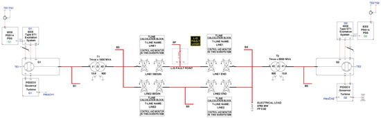
Figure 2.
Implementation in RSCAD-RTDS. PSS, Power System Stabilizer. G, Generator; B, Bus.
4.1. System Configuration
Figure 2 shows the schematic implementation of the system under study in the software RSCAD of RTDS. The system consists of two synchronous Generators G1 and G2, and their control systems (Governor PIDGOV, Automatic Voltage Regulator (AVR) EXST1, and Power System Stabilizer (PSS) STAB2A) [35,36], two three-phase transformers, two transmission lines, and an electrical load modeled as a constant impedance. The parameters of the test system can be consulted in the Appendix A.
Figure 3 presents the experimental setup of the system in RTDS. The measured three-phase voltages of buses 1, 2, 3, and 5 simulated in RTDS are sent to the PMUs. The estimated synchrophasors are sent via Ethernet in the IEEE protocol C37.118. The sample rate of synchrophasors is 60 cycles/s in protection mode. A GPS satellite clock SEL-2404 is used to timestamp the calculated phasors. All the phasors are received by a computer for further analysis.
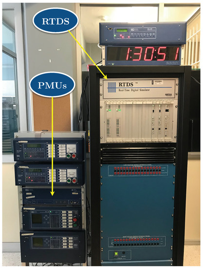
Figure 3.
Hardware-in-the-loop implementation in RTDS.
4.2. Analysis and Comparison of the Results
This section presents the analysis and comparison of the results obtained from the two simulation professional tools. To present this comparison, it the voltages at the all buses of the power system, rotor speed at the generator G1, and the angle of the voltage at bus 1 were used.
Figure 4 shows the plots, in both software, of the results of the voltages in the buses of the system. The signals have almost the same behavior, but there are some differences in the values in the first oscillations, whereas in RTDS, the value is 1.95 in p.u. at B3and in DIgSILENT PowerFactory is 1.05 p.u. These differences are due to the models used in elements such as the AVR, governors, excitation systems, synchronous machines, and transmission lines between RTDS and DIgSILENT PowerFactory. In addition, the short-circuit produced some oscillations at the beginning and at the end of the event, but as the behavior of the voltages indicated, the system was stable.
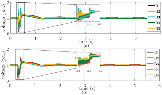
Figure 4.
Voltages in the buses of the power system: (a) RTDS. (b) DIgSILENT PowerFactory.
Figure 5 displays the rotor speed of the generator G1. It can be appreciated that both signals in RTDS and DIgSILENT PowerFactory were almost the same, but in 1.14 s, the speed in RTDS was 374.1 rad/s, while in DIgSILENT PowerFactory, it was 374.9 rad/s. In addition, the results suggest that the power system would be able to reach a new steady state, without loss of stability after being subjected to a three-phase short-circuit.
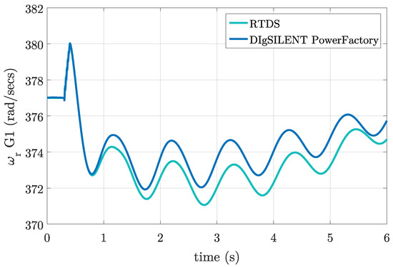
Figure 5.
Rotor speed comparison between two professional tools.
Figure 6a presents the voltage angle at bus 1 obtained from the PMUs’ SEL in radians. Figure 6b shows the same angle in degrees and referenced to the generator G1, obtained from RTDS and DIgSILENT PowerFactory, respectively. From Figure 6b, it can be observed that the signals presented the same behavior, but in detail, there were some differences; this was because the RTDS waveform was obtained directly from the industrial PMUs, while the DIgSILENT PowerFactory waveform was obtained from the RMS simulation. These signals were used to estimate the inertia for the generation unit G1.
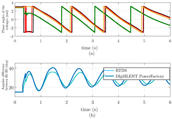
Figure 6.
Voltage synchrophasors: (a) phase angles of the voltages provided by the PMUs. (b) angular difference between Buses B1 and B5 from RTDS and DIgSILENT PowerFactory.
On the other hand, the derivative of the voltage angle on the bus followed closely the angular speed of the rotor , as shown in Figure 7. This signal was used to estimate the inertia value.
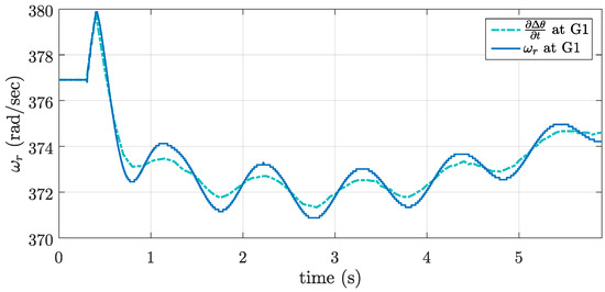
Figure 7.
Rotor speed and derivative of the angle bus in RTDS.
Table 2 presents the results of the inertia estimation for this case study. The results obtained demonstrate that there was concordance and that the results were better in comparison with the results reported in [24,25,37], where the error in the estimation was between 0.22% and 41.11%. On the other hand, [11] reported an estimation error of 16%. It is important to mention that it is not possible to establish a perfect comparison between the results obtained in this research with the results reported in the literature because the test systems were different; however, the models used and perturbations applied were similar. It is worth mentioning that the estimation errors obtained both in the literature and in this research were compared with previously-reported values, and this makes the comparison valid and fair and demonstrates that using the methodology presented in this contribution, better results were obtained.
Table 2.
Inertia estimation results at bus 1, Case 3 phase short-circuit.
In order to evaluate the accuracy and robustness of the methodology used in this paper, another case study was carried out. In this case study, in RTDS and in DIgSILENT PowerFactory, the lumped parameters PI-model for the transmission lines was used, and the generator controllers in DIgSILENT PowerFactory were tuned to obtain a similar behavior as for RTDS. Table 3 provides the results for this case study. The values obtained demonstrate robustness in the methodology to estimate the inertia in the generation units. From the results, it can be noted that the values of the inertia estimated present a considerable accuracy in comparison with the real inertia of the generation units.
Table 3.
Inertia estimation results at bus 1, Case 3 phase short-circuit and PI model.
In agreement with the results obtained in RTDS and DIgSILENT PowerFactory. It can be observed that the values were similar; this evidence suggests a considerable accuracy of the methodology for the inertia estimation values. Besides, the results validate the performance of the two professional simulation tools. In conclusion, the results and behavior of the signals are slightly different; these are due to the models used in RTDS and DIgSILENT PowerFactory. In the case of the model of the transmission lines, these differences affect the results of the voltages, currents, and the bus angle connected to these elements. Furthermore, the results shown in Table 2 and Table 3 show a considerable reliability for the use of the two professional simulation tools.
In addition, the results provided by DIgSILENT PowerFactory offer reasonable performance, so it is feasible to use this tool to estimate the inertia on large-scale power systems. An example of this affirmation is presented in the next section.
5. Inertia Estimation Varying
The results obtained using the proposed methodology demonstrate an accurate performance. However, it was observed that the accuracy of the inertia estimation depended on the increment of the total active power generated by the generation units of the system. In this section is presented a comparison of the results obtained in DIgSILENT PowerFactory with different values of to estimate the inertia at G1. The results were obtained from the experimental validation of Section 4 in the second case study. This procedure used the measurements prior to a disturbance, using different values of during the first oscillation; hence, the inertia could be estimated. Figure 8 shows the behavior of the active power provided by G1 and the inertia estimation when the short-circuit event was applied at the transmission line L1 (Figure 2).
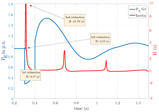
Figure 8.
Active power generated by G1 and the behavior of Hestimated.
Figure 8 presents the results of the inertia estimation when was varying. For this case study, the input inertia at G1 was H = 3.7 s; the first three approximations were H = 3.57 s, H = 13.78 s, and H = 3.13 s; and these results suggest that first approximation had a noticeable accuracy. This behavior was due to the changes of in the system and the other values used to estimate the inertia. However, this does not mean that the inertia estimation cannot be improved; some factors like the second derivate of the angle at the generation bus had an influence on the results, and its value was produced in accordance with the type of event or disturbance presented in the power system.
6. Inertia Estimation of the Southeast Zone of Mexico
An important aspect of this methodology is that it can be applied to estimate the inertia of wind power plants. Hence, this section presents the results of the methodology applied to the equivalent of the Mexican power system, in the area of the Istmo of Tehuantepec, Oaxaca, Mexico, where there is a high penetration of wind power plants.
Figure 9 shows the system presented in [38]; the system is composed of 24 wind power plants with the doubly-fed induction generator technology, and they are distributed in Ixtepec (14 wind power plants, 1438 MW) and Juchitán (10 wind power plants, 782.75 MW), with a total installed capacity of 2220.75 MW [39].
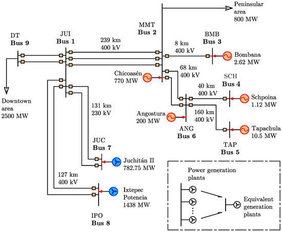
Figure 9.
One line simplified diagram of the southeast zone of Mexico.
Two case studies were carried out in the professional software DIgSILENT PowerFactory. In the first case was simulated a generation trip at bus 6, while the second case presented a load increment in the active power at bus 9.
6.1. Generation Trip at Bus 6
In this case was simulated a generation trip of 200 MW at bus 6 in 1 s. The hydropower generation units included their control systems, such as governors [40], AVR [36], and PSS [36]. The wind power plants were modeled as reported in [41,42].
Figure 10 shows the active power in p.u. at bus 3 generated by Bombana. For this case study, it can be noted that there was an increase in the value of the active power to compensate the trip generation at bus 6. A consideration previously described in the methodology to the inertia estimation was the detection of the beginning of the disturbance and the peak value of the first angular oscillation (blue window). For this case, the peak value of the active power was 0.52 p.u. in s.
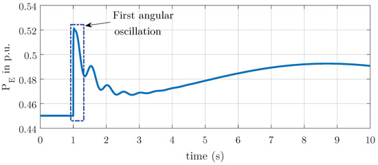
Figure 10.
Active power in p.u. at bus 3 (Bombana): generation trip case.
Table 4 summarizes the values of the estimated inertias of the generation units, where H input (s) is the inertia constant, which is already known and given by the system operator (CENACE, in English: National Energy Control Center) [40], while H estimated (s) is the inertia obtained using the methodology.
Table 4.
Inertia estimation results, generation trip case.
6.2. Load Increment
In this case study is simulated an increase in the value of the electrical load at bus 9 of 32.5 MW, in s.
Figure 11 illustrates the response of the active power at bus 2 generated by Chicoasen. It can be noted that due to the increment of the electrical load, there was an increase from 0.33 p.u.–0.3392 in p.u. in s, and this increment represents 22.5 MW of active power. The peak value was used for the inertia estimation for this generator. Furthermore, there was a minimum of oscillations when the load was increased, as a result mainly of the actions of the control systems of the generation units.
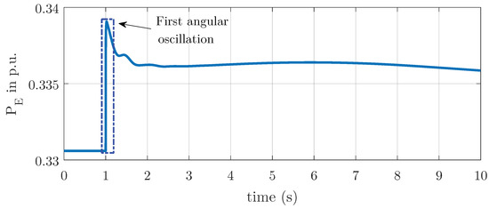
Figure 11.
Active power in p.u. at bus 2 (Chicoasen): load increment case.
Table 5 shows the results of the inertia estimation of the generation units. In particular, it can be observed that there were a few differences in the inertia estimation, and the percentage of error increased slightly in some power plants in comparison with the case study presented previously.
Table 5.
Inertia estimation results, load increment case.
This is associated with the type of disturbance applied to the power system. For this case, it was a small disturbance. Nevertheless, the results are still good in comparison with the results reported in the literature, whose values were between 0.22 %, 41.11% [24,25,37], and 16%, reported in [11].
7. Conclusions
This paper describes the experimental validation and implementation of a methodology for inertia estimation of wind power plants. This methodology is based on the equation of oscillation, and it uses measurements of the angle bus, detection of the disturbance, peak value of the disturbance, and the knowledge of active power flow in the generation units.
A comparison between the results obtained with two professional tools (RTDS and DIgSILENT PowerFactory) was carried out in order to demonstrate the accuracy, performance, and robustness of the methodology. RTDS is used for the validation of the methodology used, while DIgSILENT PowerFactory is used to calculate the inertia estimation of a large-scale power system.
Furthermore, the results of the inertia estimation of the area of the Istmo of Tehuantepec, Mexico, were analyzed and presented. From the obtained results, it can be concluded that the methodology can be applied to wind power plants. The estimation of generator inertia is accurate when a generation trip occurs in the system. However, a disadvantage of this methodology is that the accuracy is reduced when small perturbations are applied to the system. This means that the inertia estimation also depends on measurements of the disturbances and their natures.
From the results presented in this paper, it can be concluded that despite the differences between the case studies analyzed in terms of disturbances, network topology, controllers, professional tools, and modeling of the elements, the methodology presents a great robustness to obtain the inertia estimations, i.e., the results of the inertia estimation present a considerable accuracy with respect to the real inertia of the generation units.
With this methodology, it is possible to estimate the inertia in generation units, such as wind power plants, and to set the references of the synthetic inertial controllers to improve frequency stability.
Author Contributions
Conceptualization, O.B., E.M. and D.W.; Methodology, O.B., R.P., J.S., E.M. and D.W.; Software, O.B. and A.E.; Validation, O.B. and A.E.; Formal Analysis, O.B., R.P. and J.S.; Investigation, O.B., R.P., J.S., E.M. and D.W.; Data Curation, O.B. and A.E.; Writing—Original Draft Preparation, O.B., R.P. and J.S.; Writing—Review and Editing, O.B., R.P., J.S., E.M. and D.W.; Supervision, R.P.
Funding
This research received no external funding.
Acknowledgments
The authors want to acknowledge the Universidad Autonoma de San Luis Potosi through the Facultad de Ingenieria, the University of Denver, and the National Renewable Energy Laboratory (NREL) for the facilities granted to carry out this investigation. Omar Beltran Valle wants to acknowledge the financial support received from CONACYT through a scholarship to carry out his Ph.D. studies. We also thank Schweitzer Engineering Laboratories (SEL) for donating the PMU devices used to develop the case studies in real time.
Conflicts of Interest
The authors declare no conflict of interest.
Appendix A
The parameters of the single-line diagram used in this research are given in Table A1, Table A2, Table A3, Table A4 and Table A5.
Table A1.
Parameters of the synchronous generators.
Table A1.
Parameters of the synchronous generators.
| Parameter | Value | Parameter | Value |
|---|---|---|---|
| 950 (MW) | Slack | ||
| H | 3.7 (s) G1/G2 | 4.452871 (s) | |
| 13.8 | 0.252 (p.u.) | ||
| 1000 G1/5000 G2 | 0.253 (p.u.) | ||
| 0.94 (p.u.) | 0.296 (p.u.) | ||
| 0.0028544 (p.u.) | 1.305 (p.u.) | ||
| 0.06225397 (s) | 0.18 (p.u.) | ||
| 0.1 (s) | 0.474 (p.u.) |
Table A2.
Parameters of the Automatic Voltage Regulator (AVR) model used in RTDS.
Table A2.
Parameters of the Automatic Voltage Regulator (AVR) model used in RTDS.
| Parameter | Value | Parameter | Value |
|---|---|---|---|
| 200 (p.u.) | 0.1 (s) | ||
| 0 (p.u.) | 0.02 (s) | ||
| 0.001 (p.u.) | 10 (p.u.) | ||
| 0.001 (s) | -10 (p.u.) | ||
| 0 (s) | 20 (p.u.) | ||
| 0 (s) | 0 (p.u.) |
Table A3.
Parameters of the PSS model used in RTDS.
Table A3.
Parameters of the PSS model used in RTDS.
| Parameter | Value | Parameter | Value |
|---|---|---|---|
| 0.05 (p.u.) | 0.1 (p.u.) | ||
| −1 (cs) | 1 (p.u.) | ||
| 1 (MVA) | 2 (s) | ||
| 1 (p.u.) | 0.01 (s) | ||
| 0.2 (p.u.) | 0.01 (s) |
Table A4.
Parameters of the governor used in RTDS.
Table A4.
Parameters of the governor used in RTDS.
| Parameter | Value | Parameter | Value |
|---|---|---|---|
| 1 (p.u.) | 0.5 (p.u.) | ||
| 0 (p.u.) | 1 (p.u.) | ||
| 0 (p.u.) | 0 (p.u.) | ||
| 0.25 (p.u.) | 0.05 (p.u.) | ||
| 0.5 (p.u.) | 0.000001 (s) | ||
| 1.2 (p.u.) | 0.3 (s) | ||
| 0.01 (p.u.) | 0 (s) | ||
| 0 (p.u./s) | 3 (s) | ||
| 0.105 (p.u./s) | 0.1 (p.u./s) | ||
| 1.163 (p.u./s) | -0.1 (p.u./s) | ||
| 0.25 (p.u.) |
Table A5.
Parameters of the transmission lines.
Table A5.
Parameters of the transmission lines.
| Parameter | Value | Parameter | Value |
|---|---|---|---|
| R | 0.0175 (ohm/km) | 5.025292 (uS/km) | |
| 0.2758 (ohm/km) | 3.127895 (uS/km) | ||
| 0.329377 (ohm/km) | Length | 350 (km) L1/L2 | |
| 1.213911 (ohm/km) | 500 |
References
- BP-Global. Available online: https://www.bp.com/en/global/corporate/energy-economics/statistical-review-of-world-energy/renewable-energy/wind-energy.html (accessed on 8 October 2018).
- Adefarati, T.; Bansal, R. Integration of renewable distributed generators into the distribution system: A review. IET Renew. Power Gener. 2016, 10, 873–884. [Google Scholar] [CrossRef]
- Claudia, M.; Martinez, M.; Pena, R. Scenarios for a hierarchical assessment of the global sustainability of electric power plants in Mexico. Renew. Sustain. Energy Rev. 2014, 33, 154–160. [Google Scholar] [CrossRef]
- Ochoa, F.; Padilha-Feltrin, A.; Harrison, G. Evaluating distributed generation impacts with a multiobjective index. IEEE Trans. Power Deliv. 2006, 21, 1452–1458. [Google Scholar] [CrossRef]
- Saberian, A.; Farzan, P.; Nejad, M.F.; Hizam, H.; Gomes, C.; Radzi, M.A.M.; Ab Kadir, M.Z.A. Role of facts devices in improving penetration of renewable energy. In Proceedings of the IEEE Power Engineering and Optimization, Langkawi, Malaysia, 3–4 June 2013; pp. 432–437. [Google Scholar]
- Eping, C.; Stenzel, J.; Darmstadt, T.U.; Pöller, M.; Müller, H. Impact of large scale wind power on power system stability. In Proceedings of the Fifth International Workshop on Large-Scale Integration of Wind Power and Transmission Networks for Offshore Wind Farms, Glasgow, UK, 7–8 April 2005; pp. 873–884. [Google Scholar]
- Slootweg, J.; Kling, W. Aggregated modelling of wind parks in power system dynamics simulations. In Proceedings of the IEEE Power Tech Conference Proceedings, Bologna, Italy, 23–26 June 2003. [Google Scholar]
- Kundur, P.; Paserba, J.; Ajjarapu, V.; Andersson, G.; Bose, A.; Canizares, C.; Hatziargyriou, N.; Hill, D.; Stankovic, A.; Taylor, C.; et al. Definition and classification of power system stability. IEEE Trans. Power Syst. 2004, 2, 1387–1401. [Google Scholar]
- ENTSOE. European Network of Transmission System Operators for Electricity, Frequency Stability Evaluation Criteria for the Synchronous Zone of Continental Europe. RG-CE System Protection & Dynamics Sub Group, 2016. Available online: https://docstore.entsoe.eu/Docu-ments/SOC%20documents/RGCE_SPD_frequency_stability_criteria_v10.pdf (accessed on 10 November 2018).
- McLoughlin, J.; Mishra, Y.; Ledwich, G. Estimating the impact of reduced inertia on frequency stability due to large-scale wind penetration in Australian electricity network. In Proceedings of the Australasian Universities Power Engineering Conference (AUPEC), Perth, WA, Australia, 28 September–1 October 2013; pp. 1–6. [Google Scholar]
- Zhang, Y.; Bank, J.; Wan, Y.; Muljadi, E.; Corbus, D. Synchrophasor measurement-based wind plant inertia estimation. In Proceedings of the IEEE Green Technologies Conference, Denver, CO, USA, 4–5 April 2013; pp. 494–499. [Google Scholar]
- Keung, P.; Li, P.; Banakar, H.; Ooi, B. Kinetic energy of wind-turbine generators for system frequency support. IEEE Trans. Power Syst. 2009, 1, 279–287. [Google Scholar] [CrossRef]
- Frequency Task Force of the NERC Resources Subcommittee. In Frequency Response Standard Whitepaper; North American Electrical Reliability Council: Princeton, NJ, USA, 2004.
- Sharma, S.; Huang, S.; Sarma, N. System inertial frequency response estimation and impact of renewable resources in ERCOT interconnection. In Proceedings of the IEEE Power and Energy Society General Meeting, San Diego, CA, USA, 24–29 July 2011; pp. 1–6. [Google Scholar]
- Bevrani, H.; Raisch, J. On virtual inertia application in power grid frequency control. Energy Procedia 2017, 141, 681–688. [Google Scholar] [CrossRef]
- Rakhshani, E.; Remon, D.; Cantarellas, A.M.; Rodriguez, P. Analysis of derivative control based virtual inertia in multi-area high-voltage direct current interconnected power systems. IET Gener. Transm. Distrib. 2016, 10, 1458–1469. [Google Scholar] [CrossRef]
- Dreidy, M.; Mokhlis, H.; Mekhilef, S. Inertia response and frequency control techniques for renewable energy sources: A review. ELSEVIER Renew. Sustain. Energy Rev. 2013, 69, 144–155. [Google Scholar] [CrossRef]
- Longatt, F. Effects of the synthetic inertia from wind power on the total system inertia: Simulation study. In Proceedings of the International Symposium On Environment Friendly Energies and Applications (EFEA), Newcastle upon Tyne, UK, 25–27 June 2012; pp. 389–395. [Google Scholar]
- DIgSILENT. Available online: http://www.digsilent.de/ (accessed on 8 October 2018).
- Hajiakbari, M.; Esmail, M. Determining optimal virtual inertia and frequency control parameters to preserve the frequency stability in islanded microgrids with high penetration of renewables. ELSEVIER Electr. Power Syst. Res. 2018, 154, 13–22. [Google Scholar] [CrossRef]
- Fang, J.; Li, H.; Tang, Y.; Blaabjerg, F. Distributed power system virtual inertia implemented by grid-connected power converters. IEEE Trans. Power Electron. 2018, 33, 8488–8499. [Google Scholar] [CrossRef]
- D’Arco, S.; Are, J.; Fosso, O. A virtual synchronous machine implementation for distributed control of power converters in smartgrids. ELSEVIER Electr. Power Syst. Res. 2015, 122, 180–197. [Google Scholar]
- AbolhasaniJabali, M.; Kazemi, M. Estimation of inertia constant of Iran power grid using the largest simulation model and PMU data. In Proceedings of the 2016 24th Iranian Conference on IEEE Electrical Engineering (ICEE), Shiraz, Iran, 10–12 May 2016; pp. 158–160. [Google Scholar]
- Zografos, D.; Ghandhari, M.; Paridari, K. Estimation of power system inertia using particle swarm optimization. In Proceedings of the 19th International Conference on Intelligent System Application to Power Systems (ISAP), San Antonio, TX, USA, 17–20 September 2017; pp. 1–6. [Google Scholar]
- Zografos, D.; Ghandhari, M. Estimation of power system inertia. In Proceedings of the EEE Power and Energy Society General Meeting (PESGM), Boston, MA, USA, 17–21 July 2016; pp. 1–5. [Google Scholar]
- Basler, M.; Schaefer, R. Understanding power-system stability. IEEE Trans. Ind. Appl. 2008, 4, 463–474. [Google Scholar] [CrossRef]
- Kundur, P. Power System Stability and Control; McGraw-Hill: New York, NY, USA, 1994. [Google Scholar]
- Lalor, G.; Mullane, A.; O’Malley, M. Frequency control and wind turbine technologies. IEEE Trans. Power Syst. 2005, 4, 905–913. [Google Scholar] [CrossRef]
- Morren, J.; Hann, S.; Kling, W.; Ferreira, J. Wind turbines emulating inertia and supporting primary frequency control. IEEE Trans. Power Syst. 2006, 1, 433–434. [Google Scholar] [CrossRef]
- Krause, P.; Waynczuk, O.; Sudhoff, S.; Pekarek, S. Analysis of Electric Machinery and Drive Systems; Wiley-IEEE Press: Hoboken, NJ, USA, 2013. [Google Scholar]
- Ekanayake, J.B.; Holdsworth, L.; Wu, X.; Jenkins, N. Dynamic modeling of doubly fed induction generator wind turbines. IEEE Trans. Power Syst. 2003, 18, 803–809. [Google Scholar] [CrossRef]
- Mathews, J.; Fink, K. Numerical Methods Using Matlab, 4th ed.; Pearson: New York, NY, USA, 2004. [Google Scholar]
- Shetye, K.S.; Overbye, T.J.; Mohapatra, S.; Xu, R.; Gronquist, J.F.; Doern, T.L. Systematic determination of discrepancies across transient stability software packages. IEEE Trans. Power Syst. 2016, 31, 432–441. [Google Scholar] [CrossRef]
- Komal, S.; Terry, T. Assessment of discrepancies in load models across transient stability software packages. In Proceedings of the 2015 IEEE Power & Energy Society General Meeting, Denver, CO, USA, 26–30 July 2015; pp. 1–5. [Google Scholar]
- Task Force on Turbine-Governor Modeling. In Dynamic Models for Turbine-Governors in Power System Studies; The Institute of Electrical and Electronic Engineers, Inc.: New York, NY, USA, 2013.
- Energy Development and Power Generation Committee. IEEE Recommended Practice for Excitation System Models for Power System Stability Studies; The Institute of Electrical and Electronic Engineers, Inc.: New York, NY, USA, 2016. [Google Scholar]
- Ashton, P.; Taylor, G.; Carter, A.; Bradley, M.E.; Hung, W. Application of phasor measurement units to estimate power system inertial frequency response. In Proceedings of the IEEE Power Energy Society General Meeting, Vancouver, BC, Canada, 21–25 July 2013; pp. 1–5. [Google Scholar]
- Beltran, O.; Peña, R.; Segundo, J. A comparative study of the application of facts devices in wind power plants of the southeast area of the mexican electric system. In Proceedings of the IEEE International Autumn Meeting on Power, Electronics and Computing, Ixtapa, Mexico, 9–11 November 2016; pp. 1–6. [Google Scholar]
- Luna, E.; Perez, C.; Fernandez, F.; Tequitlalpa, G. Active power control of wind farms in mexico to mitigate congestion energy problems and contribute to frequency regulation. In Proceedings of the IEEE International Autumn Meeting on Power, Electronics and Computing, Ixtapa, Mexico, 5–7 November 2014; pp. 1–6. [Google Scholar]
- Centro Nacional de Control de Energia. Reglas Generales de Interconexión al Sistema Elétrico Nacional; CENACE-CFE: Mexico City, Mexico, 2012. [Google Scholar]
- Cableados Industriales. Parque eólico: Bii Nee Stipa II; Comisión Federal de Electricidad: México City, Mexico, 2010. [Google Scholar]
- DIgSILENT PowerFactory. PowerFactory User’s Manual, Version 14.0; DIgSILENT GmbH: Gomaringen, Germany, 2008. [Google Scholar]


© 2018 by the authors. Licensee MDPI, Basel, Switzerland. This article is an open access article distributed under the terms and conditions of the Creative Commons Attribution (CC BY) license (http://creativecommons.org/licenses/by/4.0/).