Online Streaming Feature Selection via Conditional Independence

Abstract

Online feature selection is a challenging topic in data mining. It aims to reduce the dimensionality of streaming features by removing irrelevant and redundant features in real time. Existing works, such as Alpha-investing and Online Streaming Feature Selection (OSFS), have been proposed to serve this purpose, but they have drawbacks, including low prediction accuracy and high running time if the streaming features exhibit characteristics such as low redundancy and high relevance. In this paper, we propose a novel algorithm about online streaming feature selection, named ConInd that uses a three-layer filtering strategy to process streaming features with the aim of overcoming such drawbacks. Through three-layer filtering, i.e., null-conditional independence, single-conditional independence, and multi-conditional independence, we can obtain an approximate Markov blanket with high accuracy and low running time. To validate the efficiency, we implemented the proposed algorithm and tested its performance on a prevalent dataset, i.e., NIPS 2003 and Causality Workbench. Through extensive experimental results, we demonstrated that ConInd offers significant performance improvements in prediction accuracy and running time compared to Alpha-investing and OSFS. ConInd offers 5.62% higher average prediction accuracy than Alpha-investing, with a 53.56% lower average running time compared to that for OSFS when the dataset is lowly redundant and highly relevant. In addition, the ratio of the average number of features for ConInd is 242% less than that for Alpha-investing.

1. Introduction

Feature selection [1,2,3,4] is the most referenced method for reducing dimensions of features. It can efficiently combat the curse of dimensionality [5] by removing irrelevant and redundant features [6]. The final goal is to extract an “optimal subset” of features from the original features [3], so that the classifiers can learn from it to improve prediction accuracy and achieve better time complexity during classification. As an important direction for feature selection, streaming feature selection (SFS) assumes that the number of training instances is fixed while the number of features increases over time [2]. For the streaming feature, features flow in one at a time, and each feature is required to be processed online upon arrival. However, all the features cannot be present in advance. Therefore, traditional batch learning that assumes that the feature selection task is conducted in an off-line learning fashion and that all features of the training instances are given a priori is not suitable [3]. Recently, online selection of dynamic features has received significant attention [7]. In some situations, online feature selection can be performed upon feature arrival where features arrive sequentially over time, especially for online feature selection with streaming features (OSFSF) that aim to provide complementary methodology for addressing high dimensional data [5]. The goal of OSFSF is to process the streaming features dynamically using the incoming streaming features one at a time [8-10]. There are several real-world application scenarios, such as streaming images captured through CCTV [11], fleeting hashtags on Twitter [12], feature collection in intrusion-detection systems [13], automatic classification of music genres in music television [14], and monitoring and analysis of environments [15]. In these applications, feature dimensions keep increasing while feature spaces become enlarged over time. Therefore, it is necessary to process online feature selection in real time to reduce processing complexity.

There are several representative research efforts on OSFSF [16], e.g., Alpha-investing, OSFS, and SAOLA, but their strategies suffer from limited prediction accuracy or running time if the streaming features possess characteristics of low redundancy and high relevance, such as in real time medical diagnosis [17]. For such streaming features, many selected features would be generated. Experiments indicate that the existing methods highlighted above are restricted to such types of streaming features. The Alpha-investing algorithm is unstable, and its prediction accuracy is significantly low on most datasets [16]. It selects numerous features from a candidate feature set because it does not re-evaluate the selected features. Hence, its performance is limited [6,16,18]. Although the OSFS algorithm offers high prediction accuracy in many datasets, its running time increases exponentially with an increase in the number of features with low redundancy and high relevance [6]. The SAOLA algorithm offers outstanding efficiency in running time and possesses few features but has low prediction accuracy [19].

To address the limitations of the abovementioned works, we propose a novel online algorithm, named ConInd, to process streaming features with low redundancy and high relevance. Unlike existing OSFSF studies, we select a subset of relevant features through three-layer filtering according to a conditional independence analysis to improve the prediction accuracy, reduce running time, and reduce the number of features selected. We use a p-value to measure the conditional independence between features within a class attribute to discard irrelevant and redundant features from candidate feature sets. In addition, we regard the subset as an approximate Markov blanket. It is well known that Markov blankets [20] provide minimal feature sets required for the classification of a chosen response variable with maximum predictability. However, it is difficult to discover unique Markov blankets in real-life datasets due to violation of the faithfulness condition [21,22]. Therefore, we only try to find an approximate Markov blanket with streaming features. Our paper mainly aims to solve the following challenges: (1) how to discover an approximate Markov blanket; (2) how to provide effective mechanisms for discovering the pattern of running times with increasing feature volumes; and (3) how to evaluate the performance of our algorithm and tackle its drawbacks.

The main contributions that distinguish the proposed method from existing methods are threefold: (1) we propose the use of a three-layer filtering strategy to process streaming features to filter irrelevant and redundant features, as presented in Section 3.2; (2) through three-layer filtering, we can obtain an approximate Markov blanket in low running time with high accuracy, as demonstrated in Section 4.3; and (3) we analyze the theoretical properties of the ConInd algorithm and validate its empirical performance by conducting an extensive set of experiments, as presented in Section 4 and Section 5.

The rest of this paper is structured as follows. Section 2 surveys related work. Section 3 introduces the preliminaries, including important notations, definitions, and a framework for filtering streaming features. Section 4 proposes our the ConInd algorithm and analyzes it. Section 5 contains our experimental results. Finally, Section 6 concludes the paper.

2. Related Work

Feature selection is a simple, interpretable and especially necessary technique for handling high dimensional data [1,3,23,24,25,26]. From the label perspective that illustrates whether label information is involved in the selection phase, feature selection includes supervised, unsupervised, and semi-supervised methods [3]. From the selection strategy perspective that describes how the features are selected, it includes wrapper methods, filter methods, and embedded methods [2,3]. OSFSF is one of the most important branches of feature selection [27]. The number of features changes over time, and it requires real time processing, rather than waiting for all features to arrive. The representative works include Grafting [28], Alpha-investing [18], OSFS [6], OGFS [29] and SAOLA [19].

Grafting [28] is an embedded feature selection approach that can discard various irrelevant and redundant features. The grafting algorithm is based on an L1 regularized formulation. It can handle streaming features but requires that the feature size be known so that it can obtain the value of the regularization parameter λ [6].

Alpha-investing [18] can handle feature sets with infinite sizes. However, it only evaluates each feature once instead of considering the redundancy of selected features. As a result, the prediction accuracy is low and unstable [5].

OSFS [6] uses the G² test to denote conditional independence or dependence and then identifies irrelevant and redundant features. OSFS can remove irrelevant and redundant features from streaming features. Therefore, it can select fewer features and obtain higher prediction accuracy than Grafting and Alpha-investing when the volume of redundant features is high. It is adaptive, enabling it to deal with extremely high dimensionality feature sets. Therefore, it guarantees that strongly relevant features and non-redundant features can be selected as the features stream one at a time as well as the removal of features that do not belong to its Marko blanket. However, with an increasing number of selected features with weak relevance, the running time grows exponentially [6].

OGFS [29] uses group structure information as a type of prior knowledge to select features. It produces improved feature subsets using two stages: intra-group feature selection and inter-group feature selection. However, OGFS needs to choose a small number of positive parameters in advance, which is relatively difficult without prior information [5].

SAOLA [19] can handle feature spaces with extremely high dimensionality using the online pairwise comparison strategy. SALOA filters out redundant features using the k-greedy search strategy, but it cannot obtain an optimal value at the same time for the relevance threshold [5].

Causal feature selection has recently been proposed as an emerging filtering approach that is successful in feature selection. In particular, the discovery of Markov blankets from Bayesian networks for feature selection has attracted much attention. Tsamardinos and Aliferis bridged the gap between the concepts of feature relevance in feature selection and Markov blanket in a Bayesian network used for classification [30]. The algorithms include the Grow–Shrink (GS) [20], the Iterative Associative Markov Blanket (IAMB) [31], HITON_MB [32], the max–min Markov blanket (MMMB) [33], the target information equivalence (TIE*) [34], and the selection via group alpha-investing (SGAI) [22].

TIE* algorithm can mine all Markov blankets under nonfaithful conditions. However, TIE* mines multiple Markov blankets for causal discovery without missing causative variables and is not yet customized for feature selection [22,34]. SGAI perform Markov blanket feature selection with representative sets for classification under the nonfaithful condition, and outperforms the state-of-the-art Markov blanket feature selectors [22].

For the above algorithms to discover Markov blankets, all features must be made available from the beginning [20]. Meanwhile, the algorithms above cannot accurately find Markov blankets, leading to the possibility that error nodes may be mined [22]. More crucially, in the context of streaming features, the features are generated dynamically and arrive one at a time. The feature selection must be done immediately in the course of generating the features. Thus, these algorithms are not suitable for mining the Markov blankets of streaming features.

Existing methods greatly relieve the burden of processing highly dimensional datasets. However, in consideration of the above limitations, we propose an efficient framework for online feature selection in a streaming feature space with low redundancy and high relevance. Based on this framework, we develop a novel algorithm called ConInd.

3. Framework for Streaming Features Filtering

3.1. Notations, Definitions, and Formalizations

The entire feature set consists of four types of features: irrelevant, redundant, weakly relevant but non-redundant, and strongly relevant features [6]. Strongly relevant features are indispensable in the sense that they cannot be removed without loss of prediction accuracy. If a strongly relevant feature is removed alone, it will result in performance deterioration of an optimal classifier. Weakly relevant features can sometimes contribute to prediction accuracy. Therefore, they are divided into non-redundant features and redundant features [6]. Irrelevant features are not necessary for improving prediction accuracy [20]. A feature is irrelevant if it is not strongly or weakly relevant [3]. Definitions of these concepts are provided in Section 3.1.2.

In the feature selection process, the features selected for class attributes include an optimal feature subset [20] that contains all non-redundant features and strongly relevant features [6]. The optimal feature subset is called the Markov blanket of class attributes. The Markov blanket criterion removes only attributes that are unnecessary, including completely irrelevant and redundant features [35].

3.1.1. Notation Mathematical Meanings

Table 1 demonstrates symbols and notations used in this paper. In the present study, we consider the problem of OSFSF for datasets with low redundancy and high relevance. S is the set of feature spaces containing all available features under the streaming feature condition. Assuming that f_i denotes the ith input feature and a new incoming feature at time t_i, CSF_i−1 is the selected feature set until time t_i−1 (CSF_i ⊂ S), and C is the class attribute [19]. Since we process one dimension at a time, the research problem at any time t_i is how to maintain a minimum size of a feature subset, S_i, online.

Table 1. Notation Mathematical meanings.

Notation	Mathematical Meanings
Xi	the data set at time ti, denoted as Xi = [x1, x2, ..., xn]T ∈ Rn×i
S	the set of feature space under the streaming features
f	a feature, f ∈ S
ti	a time point of the ith arriving feature
fi	the ith arriving feature at time ti
CFS	candidate feature set at current time
C	class attribute (target variable)
P(x)	event probability of feature x
P(.|.)	conditional probability
ρ	a threshold
α	significance levels of 0.05 or 0.01 in statistics
MB(C)	Markov blanket of C
a ⊥ b	a is independent of b

3.1.2. Definitions

Definition 1 (Conditional Independence).

In a variable set S, two random variables x, y ∈ S are conditionally independent given a set of variables $S_{\mathrm{i}}\subseteq S\backslash \{x,y\}$ with respect to a probability distribution P, iff there exists an assignment of x and y, s.t. $P(x|y,S_{\mathrm{i}})=P(x|S_{\mathrm{i}})$, denoted as $x\perp y|S_{\mathrm{i}}$.

Conditional independence is a generalization of the traditional notion of statistical independence. If two variables x and y are independent, then the joint distribution is the product of the marginal: P(x) = P(x) P(y), denoted as $x\perp y$. If they are dependent given some conditioning set, S_i, then we can write P(x,y|S_i) = P(x|S_i) P(y|S_i). Conditional independence is a key concept in Bayesian networks because of the factorizations of the allowed joint probability distribution [36].

To characterize conditional independence, according to the elements size of S_i in Definition 1, we can divide conditional independence into three disjoint categories, namely null-conditional independence (|S_i| = 0), single-conditional independence (|S_i| = 1), and multi-conditional independence (|S_i| > 1).

Definition 2 (Markov blanket).

In a variable set S, the Markov blanket of a class attribute, C, denoted as MB(C), is a minimal set of features. The MB(C) makes $\forall s\in S/(MB(C)\cup \{C\})$, s.t. $s\perp C|MB(C)$.

The Markov blanket of a node, C, denoted MB(C), is the set of parents, children, and children’s parents of C. Using the Markov blanket for feature selection can eliminate conditionally independent features without increasing our distance from the desired distribution. The Markov blanket criterion only removes attributes that are unnecessary: attributes that are irrelevant to the target variable and attributes that are redundant given other attributes [20].

Definition 3 (Strong relevance [6]).

A feature x is strongly relevant to the class attribute, C, iff$\forall S_{\mathrm{i}}\subseteq S-\left\{x\right\}$, s.t.$P(x|S_{\mathrm{i}},C)$.

Definition 4 (Weak relevance [6]).

A feature x is weakly relevant to the class attribute, C, iff $\exists S_{\mathrm{i}}\subseteq S-\left\{x\right\}$, s.t. $P(x|$$S_{\mathrm{i}},C)$.

Definition 5 (Redundant features [6])

A feature x is redundant to the class attribute, C, iff it is weakly relevant to C and has a Markov blanket, MB(x), that is a subset of the Markov blanket of MB(C).

Definition 6 (Irrelevance [6]).

A feature x is irrelevant to a class attribute, C, iff it is $\forall S_{\mathrm{i}}\subseteq S-\left\{x\right\}$, $s.t.P\left(S_{\mathrm{i}}\right|$$x,C)$$=P\left(S_{\mathrm{i}}\right|C)$.

3.1.3. Formalization of Online Feature Selection with Streaming Features

In traditional feature selection, all candidate features are available before learning starts [37,38]. For streaming features, features are generated dynamically and arrive one by one. Hence, it is not practical to wait until all features have been generated before feature selection begins [16]. In OSFSF, the data stream is fixed, whereas features keep arriving, and each feature is evaluated upon arrival. This poses great challenges to traditional feature selection approaches. A sketch of feature stream with a fixed data stream is provided in Figure 1.

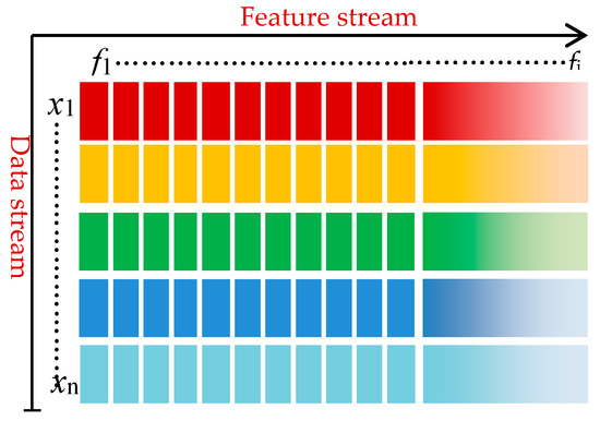
Figure 1. A feature stream with a fixed data stream.

In Figure 1, let X_i represent the data set at time t_i, denoted as X_i = [x₁, x₂, …, x_n]^T ∈ R^n×i, where n is the number of samples, i is the number of features so far over an i-dimensional feature space, and S = [f₁, f₂, …, f_i]^T ∈ Rⁱ. Let C = [c₁, c₂, …, c_m]^T ∈ R^m denote the class label vector with m distinct class labels. C denotes the class attribute, and at each time, t_i, we just obtain feature f_i of S but do not know the exact number of i in advance. Therefore, the problem is to derive x to c mapping at each time step. This is possible using a subset of the features that have arrived so far.

3.2. Framework for Filtering Conditional Independence

The feature selection process can be performed step by step, as illustrated in Figure 2, assuming that the feature space is the set of all features before the arrival of new features $f_{\mathrm{i}}$ at time $t_{\mathrm{i}}$. Of course, we do not save this space, but we filter only the new features.

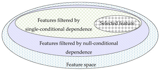
Figure 2. Features filtered using conditional dependence.

First, irrelevant features can be filtered through filtering of null-conditional dependence, leaving only relevant features. Second, parts of redundant features are further discarded from weakly relevant features through filtering of single-conditional dependence. Finally, the remaining redundant features are further filtered through filtering of multi-conditional independence. As a result, the remaining features are those that have been finally selected. The entire filtering process is repeated with the advent of new features. The arrival of new features changes the result of the selected features.

In this section, we propose a framework for filtering conditional independence to deal with data with streaming features, as illustrated in Figure 3.

Framework: The ConInd Framework

1. Initialization: class attribute C; candidate feature set: CFS; selected feature set $SF=\varnothing$; 2. Get a new feature, $f_{\mathrm{i}}$, at time ti. 3. Filtering of null-conditional independence: If $f_{\mathrm{i}}$ is an irrelevant feature, discard $f_{\mathrm{i}}$; if not, enter Step 4. 4. Filtering of single-conditional independence: Remove part of redundant features.   4.1 If $f_{\mathrm{i}}$ is a redundant feature in the filtering of single-conditional independence 1 condition, discard $f_{\mathrm{i}}$; if not, $CFS=CFS\cup \left\{f_{\mathrm{i}}\right\}$, enter Step 4.2.   4.2 If x ∈ CFS is a redundant feature in the filtering of single-conditional independence 2 condition, discard x from CFS; if not, enter Step 5. 5. Filtering of multi-conditional independence: Further remove redundant features in CFS in the filtering of the multi-conditional independence condition. 6. Repeat Steps 2–5 until there are no new features or the stopping criterion is met. 7. When SF = CFS, output the selected features, SF.

Figure 3. The ConInd framework for feature selection via conditional independence.

The following features indicate the uniqueness of the ConInd framework compared to existing algorithms. (1) ConInd employs three-layer filtering strategies with conditional independence to filter streaming features. (2) ConInd can mine an approximate Markov blanket through filtering irrelevant features and redundant features with a low time cost. At the same time, it can be used to prove the approximate Markov blanket theoretically. (3) Among algorithms for feature selection from streaming features, ConInd has significant performance improvements in terms of running time when the datasets have low redundancy and high relevance.

3.2.1. Filtering of Null-Conditional Independence

We use the filtering of null-conditional independence to identify and remove irrelevant features from streaming features. If an incoming feature is relevant to the class attribute C, the feature is added into CFS. If not, the feature would be discarded due to its irrelevance with C.

Proposition 1.

The features filtered by null-conditional independence are irrelevant features.

Proof. 

When one assumes (x, y) ∈ CFS, and considers Definitions 1 and 6, the following holds:

$$\begin{array}{ll}x\perp y|[]& \Rightarrow P(x|y,[])=P(x|[])\Rightarrow P(x|y)=P(x)\\ & \Rightarrow \frac{P(x,y)}{P(y)}=P(x)\Rightarrow P(x,y)=P(x)P(y)\Rightarrow x\perp y\end{array}$$

Therefore, x and y are non-conditionally independent and irrelevant to each other. □

3.2.2. Filtering of Single-Conditional Independence

The selected features may become redundant with time. We use the filtering of single-conditional independence to first remove parts of redundant features from a candidate feature set CFS.

The filtering of single-conditional independence is divided into two stages in order: filtering of single-conditional independence 1 and filtering of single-conditional independence 2.

Filtering of single-conditional independence 1: The single-conditional independence is filtered under the condition of each feature in the CFS. The filtering process is as follows (Figure 4):

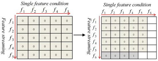
Figure 4. Filtering of single-conditional independence 1.

• Step (1): Let CFS = {f₁, f₂, f₃, f₄, f₅}; C is a class attribute, and f₆ is a new feature.
• Step (2): For each f_i ∈CFS, (i = 1, 2, …, 5), if ∃ f_i, s.t. f₆ $\perp$ C|[ f_i,], then discard f₆.
• Step (3): Else CFS = CFS $\cup$ {f₆}.
• Step (4): Return CFS.

When a new feature is added, every feature in the CFS element is used as a condition for feature selection. Once conditional independence is met, the new feature will be discarded, as illustrated in Figure 4.

Proposition 2.

C is a class attribute, $f_{\mathrm{i}}$ is a new feature at time t_i. If $\exists$ f ∈ CFS satisfies the filtering of single-conditional independence 1, i.e., $f_{\mathrm{i}}\perp C|[f]$, then f ∉ MB(C).

Proof. 

When one considers filtering of single-conditional independence 1, the following holds:

If ∃ f ∋ CFS, s.t. $f_{\mathrm{i}}\perp C|[f]$, through filtering of single-conditional independence 1, $f_{\mathrm{i}}\notin CFS$, and using Definition 2, we obtain $f_{\mathrm{i}}\in S/CFS\cup \left\{C\right\}$ s.t. $f_{\mathrm{i}}\perp C|CFS$, S is a set of the feature space, then, f_i ∉ MB(C). Therefore, Proposition 2 is proven. □

Filtering of single-conditional independence 2: The single-conditional independence is filtered on the condition of a new feature. The filtering process is as follows (Figure 5):

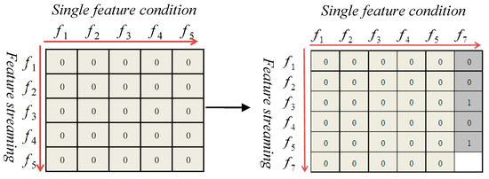
Figure 5. Filtering of single-conditional independence 2.

• Step (1): Let CFS = {f₁, f₂, f₃, f₄, f₅, f₇}, C is a class attribute, and f₇ is a new feature that is already added in the CFS through the filtering of single-conditional independence 1.
• Step (2): For each f_i (i = 1, 2, …, 5), if ∃ f_i, s.t. f_i $\perp$ C|f₇, then CFS = CFS/{f_i}.
• Step (3): Return CFS.

When a new feature is merged into CFS, it is used as a single condition to determine independence with each of the other features in the CFS. Once conditional independence is met, the other features in the CFS are discarded. For example, the features f₃ and f₅ are discarded, as illustrated in Figure 5.

Proposition 3.

C is a class attribute,$f_{\mathrm{i}}$is a new feature at time t_i,$f_{\mathrm{i}}$∈ CFS, If$\exists$f ∈ CFS/{$f_{\mathrm{i}}$}, that satisfies the filtering of single-conditional independence 2, i.e.,$f\perp C|[f_{\mathrm{i}}]$, then$f\notin MB\left(C\right)$.

Proof. 

When the filtering of single-conditional independence 2 is considered, the following holds:

If $f_{\mathrm{i}}$ is a new feature in CFS, ∃ f ∋ CFS, s.t. $f\perp C|[f_{\mathrm{i}}]$, and using Definition 2, we obtain the following:

$f_{\mathrm{i}}\in CFS$, and features in the CFS are conditionally dependent on each other, s.t. $f\perp C|CSF/\{f\}$, and f $\notin$ MB(C). Therefore, Proposition 3 is proven. □

3.2.3. Filtering of Multi-Conditional Independence

In filtering of single-conditional independence, if a feature is still not redundant, it is retained in the CFS. Therefore, we use the filtering of multi-conditional independence to identify surplus parts of redundant features in the CFS. After filtering of multi-conditional independence, the remaining features in the CFS become strongly relevant or non-redundant.

Filtering of multi-conditional independence: When a new feature is merged into the CFS, filtering of multi-conditional independence is started. The filtering steps are as follows:

• Step (1): C is a class attribute; for each f ∈ CFS, S_i $\subseteq$ CFS/{f},
• if ∃ S_i, s.t. f $\perp$ C|S_i, then CFS = CFS/{f}.
• Step (2): If $\forall$f ∈ CFS, S_i $\subseteq$ CFS/{f}, s.t. f $\bcancel{\perp }$ C|S_i, return CFS.

Proposition 4.

For a class attribute, C, the candidate feature set CFS goes through filtering of multi-conditional independence. If$\forall$f ∈ CFS,$\forall$S_i$\subseteq$CFS/{f}, s.t.$f\bcancel{\perp }C|S_{\mathrm{i}}$, then, f ∈ MB(C).

Proof. 

Suppose CFS has already been filtered through the filtering of multi-conditional independence. $\forall$f ∈ CFS, $\forall$S_i $\subseteq$ CFS/{f}, s.t. $f\bcancel{\perp }C|S_{\mathrm{i}}$. Because the MB (C) is a subset of CFS, $\exists$S_i = MB (C), s.t. $f\bcancel{\perp }C\left|MB\right(C)$. According to Definition 2, if $f\perp C|MB(C)$, f $\notin$ MB (C). Therefore, f ∈ MB(C). □

4. Online Streaming Feature Selection Algorithms

4.1. The ConInd Algorithm and Analysis

The ConInd framework is used with online feature selection for filtering of streaming features. We provide the detailed proposal of the ConInd algorithm, as illustrated in Figure 6. In the ConInd algorithm, CFS is a candidate feature set of current time, whereas $f_{\mathrm{i}}$ is a new feature at time t_i.

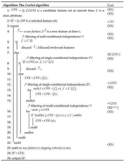
Figure 6. The ConInd algorithm.

Filtering 1:Filtering of null-conditional independence: In Steps 5 and 6, the filtering of null-conditional independence is executed. If $f_{\mathrm{i}}$ is an irrelevant feature with a class attribute C, the feature $f_{\mathrm{i}}$ is discarded. Otherwise, the feature $f_{\mathrm{i}}$ is further used in the filtering of single-conditional independence.

Filtering 2:Filtering of single-conditional independence: The filtering of single-conditional independence is orderly divided into two step categories: Steps 8–11 involve the filtering of single-condition independence 1, whereas Steps 12–15 involve the filtering of single-condition independence 2.

• Filtering of single-conditional independence 1: For each feature in the CFS, we determine the conditional independence with the class attribute C. If $\exists f\in CFS,$ $s.t.$ $f_{\mathrm{i}}\perp C|[f]$, then discard $f_{\mathrm{i}}$, because it is a redundant feature. Next, jump to Step 3 and continue to determine the next new feature $f_{\mathrm{i}+1}$. On the contrary, if $\exists f\in CFS,$ $s.t.$ $f_{\mathrm{i}}\bcancel{\perp }C|[f]$, then feature $f_{\mathrm{i}}$ is non-redundant with the class attribute C. The feature $f_{\mathrm{i}}$ is then included in the CFS. It is validated through the filtering of single-conditional independence 2.
• During the filtering of single-conditional independence 2: For the new feature $f_{\mathrm{i}}$, the conditional independence of each feature in the CFS expected for $f_{\mathrm{i}}$ is determined one feature at a time. If $f\in CFS-\left\{f_{\mathrm{i}}\right\}\mathrm{s}.\mathrm{t}.f\perp C|[f_{\mathrm{i}}]$, discard f from CFS and jump to Step 3. The reason is that f and C are conditionally independent under the condition of $f_{\mathrm{i}}$. Therefore, the feature f is unnecessary if $f_{\mathrm{i}}$ ∈ CFS. On the contrary, if $f\in CFS-\left\{f_{\mathrm{i}}\right\}$, $s.t.$ $f\bcancel{\perp }$ $C|[f_{\mathrm{i}}]$, the feature $f_{\mathrm{i}}$ is kept in the CFS. Then, we continue filtering for multi-conditional independence.

Filtering 3:Filtering of multi-conditional independence: As indicated in Steps 16–20, for the CFS, each feature f in the CFS, $y\perp C|subSet$, is determined under the condition of $subSet\subseteq CFS-\left\{y\right\}$. If $y\perp C|subSet$, then feature y is redundant and is discarded from CFS. Through a continuous loop in Steps 16–20, all redundant features in the CFS are discarded due to the arrival of new features.

The ConInd algorithm uses the notation $f_{\mathrm{i}}\perp C|S$, S $\subseteq$ CFS − {$f_{\mathrm{i}}$}, to denote conditional independence. To evaluate $f_{\mathrm{i}}\perp C|S$, ConInd uses the p-value returned by the G² test for discrete data and Fisher’s z-test for continuous data to measure it, with a significance level of 0.05 or 0.01 often used. In the present study, we set the significance level threshold value to 0.05.

Assuming that α is a given significance level of 0.05 and ρ is the p-value returned, $f_{\mathrm{i}}\perp C|S$ defines the null hypothesis (H₀). $f_{\mathrm{i}}$ and C are conditionally independent given S, iff ρ > α. $f_{\mathrm{i}}\bcancel{\perp }C|S$ defines the alternative hypothesis (H₁). $f_{\mathrm{i}}$ and C are non-conditionally independent given S, iff ρ ≤ α.

4.2. The Time Complexity of ConInd

The complexity of the ConInd algorithm depends on the test of null-conditional, single-conditional, and multi-conditional independence. It is assumed that |N| is the number of features that have arrived so far, |N_i| is the number of irrelevant features with the class attributes that have arrived so far, |M| is the number of remaining features before multi-conditional independence filtering, and |CSF| is the size of candidate feature sets that have arrived so far, as illustrated in Figure 6.

Table 2 presents that the time complexity of filtering of single-conditional independence is obviously lower than multi-conditional independence with increasing |CFS|. The key advantage of the ConInd algorithm is that, in the phase of filtering single-conditional independence, some redundant features are filtered. Objectively, |CFS| and |M| become smaller in the phase of filtering multi-conditional independence, and the time complexity, O(|M||CFS|2^|CFS|), is significantly reduced.

Table 2. The time complexity in the phase of three-layer filtering.

Phase of Filtering	Cost
null-conditional independence	O(|N|)
single-conditional independence	O((|N| − |Ni|)|CFS|)
multi-conditional independence	O(|M||CFS|2|CFS|)

The time complexity of ConInd is O(|N| + (|N| − |N_i|)|CFS| + |M||CFS|2^|CFS|). The time complexity of ConInd is mainly determined by the parameters |N|, |N_i|, |M|, and |CFS|. If most elements in the feature set are irrelevant features, the time complexity of ConInd becomes close to O(|N|). |M| and |CFS|, particularly |CFS|, have the greatest impact on the ConInd algorithms. In general, the value of |CFS| is far less than |N| − |N_i|, and |N|, (|CFS| < |M| < |N| − |N_i| < |N|). Through three-layer filtering, it can be ensured that |M| is not very large. We will discuss the details in Section 5.2. With the continuous arrival of strong relevance features, the complexity of ConInd becomes very high. The larger the volumes of irrelevant and redundant features are, the faster the ConInd algorithm is. The worst-case complexity is O(|N| + |N||CFS| + |N||CFS|2^|N|), where the size of the feature within the CFS is |N| in Step 17. Of course, this situation rarely exists.

4.3. Analysis of Approximate Markov Blankets of ConInd

We mine an approximate Markov blanket of the streaming feature for the following reasons: (1) To guarantee that the class attribute has a unique Markov blanket, the distribution of the dataset must be faithful [20,35]. However, many datasets from real-world applications may violate the faithful condition, and this makes the Markov blanket of a class attribute to be not unique [22]. (2) An optimal feature selection should select strongly relevant and non-redundant relevant features. However, as features continuously arrive in a streaming fashion, it is difficult to find all the strongly relevant and non-redundant features [3]. Therefore, we only attempt to find an approximate Markov blanket.

Through three-layer filtering, the ConInd algorithm discards many features from the CFS. The remaining features constitute elements of the selected feature set. According to Propositions 1–4, the discarded features do not belong to the Markov blanket of a class attribute. Obviously, the ConInd algorithm cannot move strongly relevant or non-redundant relevant features from the CFS. The ConInd algorithm can discard as many irrelevant and redundant features as possible. The set of selected features is called an approximate Markov blanket.

5. Experiments and Analysis

5.1. Experimental Setup

We empirically evaluated the performance of the algorithms. All experiments were conducted on a computer with Intel (R) Xeon (R) CPU E3-1505M 3.0 GHz, 32 GB RAM.

We tested representative algorithms of Alpha-investing and OSFS on the 14 benchmark datasets in Table 3. The arcene, colon, ionosphere, and leukemia datasets come from the NIPS 2003 feature selection challenge [8] and one frequently studied public microarray dataset (wdbc). We also downloaded the datasets from Causality Workbench, such as slyva, lung, cina0, reged1, lucas0, marti1, and lucap0. Cina0 is a marketing dataset derived from census data while reged1 is a genomics dataset that could be responsible for lung cancer. Marti1 is obtained from the data generative process of simulated genomic data. Lucas0 is a lung cancer simple set, whereas lucap0 is a lung cancer set with probes. They are used to model a medical application for the diagnosis, prevention, and cure of lung cancer. The number of features ranges from 11 to 10,000, and the number of samples varies from 72 to 145,252. In particular, the number of features in seven datasets—marti1, reged1, lung, prosate_GE, leukemia, arcene, and Smk_can_187—is larger than the number of samples. These 14 datasets cover a wide range of real-world application domains, including gene expressions, ecology, and casual discovery. This makes the construction of feature selection extremely challenging. We preprocessed the data, for example deleting similar columns in the leukemia dataset.

Table 3. Summary of the benchmark datasets.

Datasets	#	Size	Dataset	#	Size
wdbc	30	569	marti1	1024	500
colon	2000	62	reged1	999	500
lucas0	11	2000	lung	3312	203
sylva	216	13,086	prosate_GE	5966	102
ionosphere	34	351	leukemia	7066	72
cina0	132	16,033	arcene	10,000	100
lucap0	143	2000	Smk_can_187	19,993	187

#, the number of features, Size, the number of instances.

Our comparative study had the following design and compares the ConInd algorithm with two state-of-the-art online feature selection algorithms, namely Alpha-investing and OSFS, using 10-fold cross validation on each training dataset. The experiment was traced as follows: (1) analyzing the change in the number of features at every stage of running the ConInd; (2) comparing the prediction accuracy of ConInd with Alpha-investing and OSFS through some state-of-the-art classifiers, including Decision Tree, KNN, SVM, and Ensemble using their implementation provided in the MATLAB app tool; (3) analyzing the number of selected features and running time in different algorithms; and (4) analyzing changing trends in the numbers of selected features and running time in different ratios of the streaming features.

5.2. Number of Features through Filtering of Conditional Dependence in the ConInd Algorithm

To observe the variation of number of features through every filtering phases, i.e., null-conditional independence, single-conditional independence, and multi-conditional independence, Table 4 summarizes the variation of number of features with the three-layer filtering of conditional independence in ConInd algorithm.

Table 4. The number of features in filtering conditional independence.

Datasets	Number of Features (#)
	#IFS	#NIC	#SIC	#MIC (SF)
wdbc	30	24	6	3
colon	2000	359	5	3
lucas0	11	9	4	4
sylva	216	77	52	24
ionosphere	34	25	7	5
cina0	132	106	57	30
lucap0	143	94	49	40
marti1	1024	1	1	1
reged1	999	541	16	13
Lung	3312	2318	212	35
prosate_GE	5966	3182	24	4
leukemia	7066	2019	47	8
arcene	10,000	2666	13	6
Smk_can_187	19,993	4924	55	9

#, the number of selected features; #IFS, the number of initial feature space; #NIC, # via the filtering of Null-conditional dependence; #SIC, # through the filtering of Single-conditional dependence; #MIC, # through the filtering of Multi-conditional dependence; SF, selected feature of running algorithm.

In Table 4, we can observe that the elements of the candidate feature set gradually decrease under the three-layer filtering of conditional dependence. The filtering efficiency of ConInd increases with variation of feature number in the CFS. Moreover, the higher the dimension is, the more obvious the effect of ConInd is because, with the increase of feature scale, irrelevant features and redundant features will rapidly increase. For the five datasets of sylva, cina0, lucap0, reged1, and Lung, the number of selected features in the SF is greater than 10. This is because there are many features that are strongly relevant with class attribute in these datasets. For such datasets, the ConInd algorithm often has shorter running time than OSFS, especially for the datasets highlighted in bold. The reason is that most of the features have been filtered by the filtering of single-conditional independence. In the multi-conditional filtering phase, the size of filtering condition is relatively smaller than OSFS. We discuss the details in Section 5.3.2.

5.3. Comparison of ConInd with Two Online Algorithms

The above algorithms were all implemented in LOFS (Library of Online streaming Feature Selection) [39], an open-source library of online feature selection streaming features in MATLAB. To evaluate selected features in the experiments, we used the following 12 classifiers: Decision Tree (Complex Tree, Medium Tree, and Simple Tree), SVM (Linear SVM, Quadratic SVM, and Cubic SVM), KNN (Fine KNN, Medium KNN, and Cubic KNN), and ENSEMBLE Classifiers (Bagged Trees, Subspace discriminant, and RUSBoosted Trees). The classifiers were integrated into the MATLAB app tool.

To compare the performance of the proposed ConInd with existing streaming feature selection methods, we evaluated ConInd and its rivals based on prediction accuracy, sizes of selected feature sets, and running time. In the remaining sections, we present the following statistical comparisons to further analyze the prediction accuracy of ConInd.

5.3.1. Prediction Accuracy

As illustrated in Figure 7, we summarize the prediction accuracy for the 12 classifiers on the 14 datasets during online learning. The labels of the x-axis from 1 to 14 denote the datasets: (1) wdbc; (2) colon; (3) lucas0; (4) sylva; (5) ionosphere; (6) cina0; (7) lucap0; (8) marti1; (9) reged1; (10) Lung; (11) prosate_GE; (12) leukemia; (13) arcene; and (14) Smk_can_187.

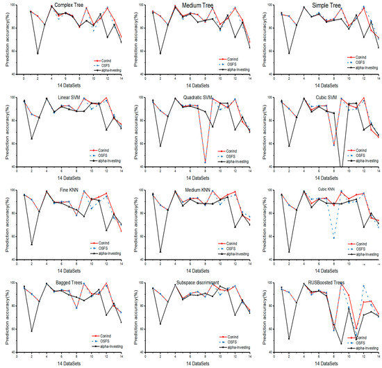
Figure 7. Prediction accuracy of algorithms in the 14 datasets under different classifiers.

We conducted experiments on these datasets using G² tests for discrete data and Fisher’s Z-test for continuous data at a significance level α = 0.05. The prediction accuracies of ConInd and OSFS were higher than that of Alpha-investing on 5–14 datasets in these classifiers. ConInd consistently achieved higher accuracy in all classifiers except for RUBSBoosted Trees. As shown in Figure 7, the accuracies of the classifiers were overtly reduced in the leukemia, marti1, and reged1 datasets. As shown in the three curves in Figure 7, we observed that Alpha-investing, OSFS, and ConInd have the same prediction accuracies in some datasets. There are seven datasets in ComplexTree, two in Medium Tree, four in SimpleTree, five in Liner SVM, four in Quadratic SVM, four in Cubic SVM, five in FineKNN, four in Medium KNN, four in Cubic KNN, four in Bagged Trees, four in Subspace discriminant, and three in RUBSBoosted Trees. Prediction accuracies for the wdbc, lucas0, and sylva datasets were equal, except for RUBSBoosted Trees, because they have the same respective selected features.

Table 5 presents the results of average accuracy in three different algorithms for the 14 datasets. For the average of Decision Tree, SVM, KNN, and ENSEMBLE, ConInd offers higher average accuracy (i.e., 88.79, 88.63, 9.76, and 88.61, respectively) than Alpha-investing (i.e., 83.74, 84.08, 83.2, and 82.3, respectively) does. The average classification accuracy of the features selected using the ConInd algorithm is the highest among the three algorithms. It is important to note that the average accuracy of ConInd is 5.62% higher than that of Alpha-investing.

Table 5. Comparison of average prediction accuracies.

Algorithms	Average Accuracy for Classifiers in 14 the Datasets (%)						Average Accuracy (%)
Alpha-investing	Complex Tree	Medium Tree	Simple Tree	Linear SVM	Quadratic SVM	Cubic SVM	83.33
	83.89	84.14	83.18	86.34	85.13	80.78
	Decision Tree average: 83.74			SVM average: 84.08
	Fine KNN	Medium KNN	Cubic KNN	Bagged Trees	Subspace discriminant	RUSBoosted Trees
	82.31	83.75	83.54	84.91	86.19	75.81
	KNN average: 83.2			ENSEMBLE average: 82.3
OSFS	Complex Tree	Medium Tree	Simple Tree	Linear SVM	Quadratic SVM	Cubic SVM	88.44
	88.22	88.58	88.62	90.44	87.60	87.64
	Decision Tree average: 88.47			SVM average: 88.56
	Fine KNN	Medium KNN	Cubic KNN	Bagged Trees	Subspace discriminant	RUSBoosted Trees
	87.83	90.22	87.41	89.89	90.27	84.54
	KNN: 88.49			ENSEMBLE: 88.23
ConInd	Complex Tree	Medium Tree	Simple Tree	Linear SVM	QuadraticSVM	Cubic SVM	88.95
	89.14	89.19	88.05	90.94	87.50	87.46
	Decision Tree average: 88.79			SVM average: 88.63
	Fine KNN	Medium KNN	Cubic KNN	Bagged Trees	Subspace discriminant	RUSBoosted Trees
	88.79	90.42	90.07	90.05	90.63	85.14
	KNN average: 89.76			ENSEMBLE average: 88.61

In our experiments, we found that ConInd has better accuracy than Alpha-investing. As mentioned above, this is because Alpha-investing only evaluates each feature once instead of considering the redundancy of selected features. As a result, the prediction accuracy is low and unstable. Similarly, ConInd also shows slightly better average accuracy than OSFS. A possible explanation is that a few parts of strongly relevant features and non-redundant features may be discarded due to the characteristics of streaming features.

5.3.2. The Number of Selected Features and Running Time

To further analyze the performance of the three algorithms in the number of selected features and running time, Table 6 presents their performances in the 14 datasets.

Table 6. The number of selected features and running time.

Datasets	Algorithms
	Alpha-investing		OSFS		ConInd
	#	Time	#	Time	#	Time
wdbc	20	0.0138	3	0.1577	3	0.2201
colon	1	0.0663	3	0.6778	3	8.6637
lucas0	4	0.0008	4	0.0142	4	0.0304
sylva	70	1.6717	18	247.9366	24	189.8111
ionosphere	10	0.0147	4	0.1315	5	0.2215
cina0	8	0.1046	22	721.3638	30	407.7689
lucap0	10	0.0197	36	1.67 × 103	40	225.7368
marti1	28	0.116	1	0.1081	1	0.1063
reged1	1	0.0417	13	121.2839	13	63.9082
lung	45	0.7523	11	420.5678	35	3.48 × 104
prosate_GE	12	0.4308	3	7.7915	4	4.72 × 104
leukemia	1	0.4346	3	12.7647	8	593.3249
arcene	8	1.4139	5	20.8445	6	764.5764
Smk_can_187	6	2.7929	4	42.8323	9	327.1579
the ratio of average features number: $({{\displaystyle \sum \#}}_A-{{\displaystyle \sum \#}}_C)/{{\displaystyle \sum \#}}_C$ = 242%

#, the number of selected features; Time, running time; ${{\displaystyle \sum \#}}_A$ and ${{\displaystyle \sum \#}}_C$, respectively, the sum of # of Alpha-investing and ConInd.

• A summary of the number of selected features of the algorithms

As shown in Figure 7, we observed that the prediction accuracy of ConInd is higher than that of Alpha-investing and OSFS for most of the datasets. However, in Table 6, it is obvious that the number of selected features is greater in Alpha-investing than in ConInd and OSFS for many datasets. In the 14 datasets, the ratio of the average number of features for Alpha-investing is 242% higher than that for ConInd. The can be attributed to the following reasons:

(a)

The predictive accuracy of Alpha-investing is low. This means that a part of the elements in Markov blanket cannot be obtained.

(b)

For the OSFS algorithm, during the redundant feature analysis phase, it is possible that non-redundant features are discarded under the condition of redundant features, resulting in low predictive accuracy and fewer features being selected.

(c)

For the ConInd algorithm, there are two aspects that account for the large number of selected features. On the one hand, ConInd significantly outperforms OSFS and Alpha-investing in mining the elements in the Markov blanket. It can find many more elements than OSFS in the Markov blanket. On the other hand, the number of #SIC is much smaller than the number of #NIC, as presented in Table 4. This also means that the size of the feature subset for the #SIC condition is smaller than the subset of #NIC. Therefore, there is a low possibility that the feature can be discarded.

• A summary of running time of algorithms

A summary of the performance of three algorithms in terms of running time is reported in Table 6. Obviously, Alpha-investing is much faster than OSFS and ConInd for all datasets. This is because Alpha-investing considers only new features that are added; the discarded features are never considered again. This also leads to generally low prediction accuracy (Figure 7), such as those for colon, lucap0, reged1, leukemia, and Smk_can_187 classifiers.

The performances of ConInd and OSFS in terms of running time are significantly different. The results in Table 6 indicate that OSFS is much faster than ConInd on datasets wdbc, colon, lucas0, ionosphere, lung, prosate_GE, arcene, leukemia, and Smk_can_187. Conversely, ConInd is much faster than OSFS on datasets sylva, cina0, lucap0, and reged1. These datasets are highlighted in bold. The differences arise from the feature relevance and the redundancy of the datasets. We find that the datasets in bold have more selected features (as indicated in Column 6 of Table 6); these datasets have low redundancy and high strong and weak relevance because the runtime for the two algorithms is significantly influenced by the size of candidate selected features.

Table 7 presents that, when the datasets are lowly redundant and highly relevant, the average running time for ConInd is reduced by 53.56% compared to OSFS. This indicates that ConInd has perfect efficiency in terms of running time.

Table 7. Variation in the ratio of running time for Alpha-investing and ConInd.

Datasets	Running Time		$\mathit{A}{\mathit{v}}_{\mathit{T}}(\%)$	$\mathit{A}\mathit{v}\mathit{e}\mathit{r}\mathit{a}\mathit{g}\mathit{e}\mathit{A}{\mathit{v}}_{\mathit{T}}$
	TA	TC
sylva	247.9366	189.8111	−0.2344	−0.5356
cina0	721.3638	407.7689	−0.4347
lucap0	1.43 × 107	225.7368	−0.9998
reged1	121.2839	63.9082	−0.4731

T_A, running time of Alpha-investing; T_C, running time of ConInd; $A{v}_T=(T_A-T_C)/T_A$, variation in the ratio of the running time.

5.3.3. Variation in the Number of Features and Running Time with the Increase of Feature Ratio

To further observe the variation in of number of features and running time in every filtering phase with the increase of the feature size, we ran these algorithms by step by step increasing the features size in 14 datasets.

In the experiment, the running time was reported as execution time only. For comparison, all datasets were executed once in the same environment. We observed the variation ratio of the feature number by continuing to increase the incoming features from 20% to 100%, as presented in Table 8.

Table 8. Variation in the number of selected features and running time with the ratio of feature space.

Dataset	Ratio	#				Time
		ConInd			OSFS	ConInd	OSFS
		#NIC	#SIC	SF	SF
ionosphere	25%	8	5	5	4	0.0222	0.0184
	50%	15	6	5	4	0.0855	0.0678
	75%	21	6	5	4	0.148	0.1078
	100%	25	7	5	4	0.2215	0.1315
marti1	25%	0	0	0	0	0.0235	0.0251
	50%	0	0	0	0	0.0446	0.0474
	75%	0	0	0	0	0.0673	0.0698
	100%	1	1	1	1	0.1063	0.1081
leukemia	25%	488	21	5	3	74.3909	3.6738
	50%	914	28	6	3	143.903	5.8859
	75%	1521	35	8	4	356.6957	9.9276
	100%	2019	47	9	3	593.3249	12.7647
arcene	25%	670	3	3	4	26.9589	1.6326
	50%	1354	8	5	4	111.864	6.8246
	75%	2017	11	6	3	259.0335	10.2471
	100%	2666	13	6	5	764.5764	20.8445
cina0	25%	24	17	12	10	3.6124	3.8368
	50%	52	30	17	14	34.372	35.8382
	75%	81	47	28	23	157.9134	263.1822
	100%	106	57	30	22	407.7689	721.3638
sylva	25%	22	17	12	10	4.3963	12.7006
	50%	36	24	15	13	13.3102	27.0316
	75%	55	39	22	18	53.8118	115.1798
	100%	77	52	24	18	189.8111	247.9366
lucap0	25%	24	18	16	15	2.4505	10.5797
	50%	50	38	32	26	32.2265	147.5867
	75%	68	44	36	30	88.2781	416.6544
	100%	94	49	40	36	225.7368	1.43 × 107
reged1	25%	6	1	1	2	0.0282	0.0299
	50%	15	3	3	4	0.0791	0.103
	75%	22	5	5	6	0.1639	0.2067
	100%	541	16	13	13	63.9082	121.2839

Ratio, ratio of feature space #, the number of selected features; Time, runtime; Ratio, Ratio of feature number; SF, selected feature of the algorithm; #NIC, # through the filtering of null-conditional dependence; #SIC, # through the filtering of single-conditional dependence.

At a ratio of 100% for incoming features, the changes in the features by filtering for the cina0, sylva, lucap0, and reged1 datasets were 106 → 57 → 30, 77 → 52 → 24, 94 → 49 → 40, and 541 → 16 → 13 (Table 8). We observed that, from #NIC → #SIC → SF, there was a low range in the number of features, and more than 10 features were selected. This means that the datasets have low redundancy and high relevance. Similarly, we observed that, in the datasets for leukemia and arcene, the change of features by filtering was 2009 → 47 (2.3%) and 2666 → 13 (0.48%). The number of features declined rapidly, meaning that the features are highly redundant. For the datasets of ionosphere and marti1, the number of relevant features was only 25 and 1, respectively. Therefore, the running time for OSFS was lower than that for ConInd. This is because the filtering for single-conditional independence is not necessary for a few non-redundant features. For the first four datasets in Table 8, OSFS significantly outperformed ConInd over many datasets in terms of the number of selected features and running time. By contrast, it was observed that, to the right of the data in Table 8, ConInd significantly outperformed OSFS. The best result for the ConInd algorithm is highlighted in bold on the right side of Table 8. The representative datasets include sylva, cina0, lucap0, and reged1. The results indicate that the ConInd algorithm achieved better results than OSFS in candidate feature sets with low redundancy and high relevance. OFSF is suitable for high redundancy feature streaming and spare candidate feature sets. The encouraging results verify the efficacy of the ConInd algorithm for datasets with low redundancy and high relevance.

As illustrated in Figure 8, ConInd outperformed OSFS on the cina0, sylva, lucap0, and reged1 datasets. As the size of the features increased, the running time for OSFS increased rapidly, while the running time for ConInd remained stable. It can also be seen in Table 8 that the four datasets have very few redundant features. Meanwhile, there is higher number of SF in the two algorithms. The number of SF was more than 10, e.g., for OSFS, 18 for sylva, 22 for cina0, 36 for ucap0, and 13 for reged1. For ConInd, the number change from #SIC to SF was 52 → 24, 57 → 30, 49 → 40, and 16 → 13 for the sylva, cina0, lucap0, and reged1 datasets, respectively.

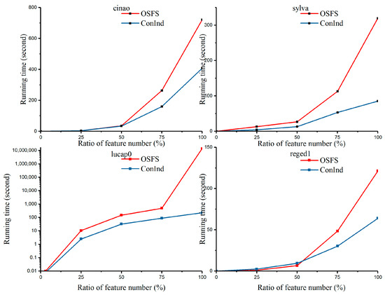
Figure 8. The variation in running time with increase in ratio feature number in datasets with low redundancy and high relevance.

As illustrated in Figure 9, OSFS outperformed ConInd on the ionosphere, leukemia, marti1, and arcene datasets. The running time for OSFS remained stable as the size of the features increased, while the running time for ConInd increased rapidly. It can also be seen in Table 8 that the four datasets have very few features in SF or many redundant features. Meanwhile, the number of SF for the two algorithms was less than 10; e.g., for OSFS, there are four for ionosphere, three for leukemia, one for marti1, and five for arcene. For ConInd, the number variation from #SIC to SF was 7 → 5, 47 → 8, 1 → 1, and 13 → 6 for the ionosphere, leukemia, marti1, and arcene datasets, respectively.

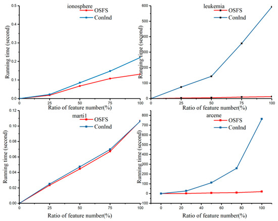
Figure 9. The variation of running time with the increase of ratio feature number with high redundancy and low relevance.

To sum up, Figure 8 shows that ConInd significantly improves performance in the aspect for running time while the datasets is lowly redundant and highly relevant. This is because the number of selected features is quite large in these datasets. This means that, compared with ConInd, OSFS will spend more time dealing with redundant features. In contrast, Figure 9 shows that, with the increase of feature size, ConInd is not suitable for processing the datasets with high redundancy and low relevance. The reason is that the filtering of single-conditional independence would spend some time. Instead, when the number of selected features is very small, OSFS uses very little time to process redundant features. Therefore, from the perspective of time performance, ConInd is more suitable for dealing with the datasets with low redundancy and high relevance.

5.4. Comparison of ConInd with Two Markov Blanket Algorithms

To observe the performance of the proposed ConInd algorithm in the aspect of mining Markov blankets, we compared ConInd with other methods of discovering Markov blankets, i.e., HITON_MB and OSFS. The HITON_MB is the first concrete algorithm that would find sets of direct causes or direct effects and Markov blankets in a scalable and efficient manner [20]. However, some error nodes may be introduced. The OSFS algorithm contains online relevance analysis and online redundancy analysis based on a Markov blanket criterion. The redundant features removed earlier remain redundant during the rest of the process when some features within its Markov blanket are later removed [16]. There is a distinct difference between these two families of algorithms: HITON_MB can only handle fixed feature sets. Therefore, we fixed feature sets instead of streaming features. The Probabilistic Network Learning Toolkit for Biomedical Discovery (Causal Explorer) [31] is the first comprehensive library for use in MATLAB that implements the HITON_MB algorithms for discovering Markov blankets. Meanwhile, ConInd and OSFS run datasets with streaming features. To compare HITON_MB with ConInd and OSFS, it is interesting and useful to compare them directly. According to the results of the algorithm, we mainly analyzed the following aspects: (1) degree of closeness among HITON_MB, OSFS, and ConInd; and (2) the reasons for the differences in the results of the Markov blankets.

Table 9 presents the results of the number of selected features for ConInd, HITON_MB, and OSFS. We observed that HITON_MB has more selected features than those in ConInd and OSFS. This is because HITON_MB discovers the Markov blanket under fixed features, and mined features may not belong to nodes in its Markov blanket. Meanwhile, many error nodes will be produced in HITON_MB.

Table 9. The number of selected features of the three algorithms.

Dataset	HITON_MB	OSFS	ConInd
wdbc	5	3	3
colon	3	3	3
lucas0	5	4	4
sylva	64	18	24
ionosphere	6	4	5
cina0	66	22	30
lucap0	79	36	40
marti1	3	1	1
reged1	24	13	13
lung	97	11	35
prosate_GE	6	3	4
leukemia	7	3	8
arcene	8	5	6
Smk_can_187	11	4	9

Table 5 and Table 10 present the results of comparison of prediction accuracy. Although the number of selected features for ConInd is far less than that of HITON_MB, as indicated in Table A1, the prediction accuracies of ConInd are not significantly lower than those of HITON_MB. Meanwhile, these selected features for ConInd are approximately included in HITON_MB. Meanwhile, these features are indispensable to classification and prediction, and are strongly relevant or non-redundant to class attribute.

Table 10. Average prediction accuracies of HITON_MB.

Algorithms	Average Accuracy for Classifiers in the 14 Datasets (%)						Average Accuracy (%)
HITON_MB	Complex Tree	Medium Tree	Simple Tree	Linear SVM	Quadratic SVM	Cubic SVM	89.51
	88.54	88.74	88.80	92.76	91.78	87.59
	Decision Tree average: 88.69			SVM average: 90.71
	Fine KNN	Medium KNN	Cubic KNN	Bagged Trees	Subspace discriminant	RUSBoosted Trees
	89.11	90.98	90.56	88.61	91.61	85.00
	KNN average: 90.22			ENSEMBLE average: 88.41

6. Conclusions

We studied the online feature selection problem with streaming features. By employing multi-layer filtering strategies with conditional independence, we proposed an online learning algorithm called ConInd to reduce the dimensionality of streaming features by removing irrelevant and redundant features in real time.

The proposed ConInd algorithm can output an approximate Markov blanket in a short running time, with high accuracy even when the streaming features have low redundancy and high relevance. Our empirical study demonstrated that: (1) ConInd has significant performance improvements in terms of accuracy prediction compared to Alpha-investing and OSFS. The average increase in accuracy prediction was 5.62% higher than that of Alpha-investing and 0.51% higher than that of OSFS. (2) ConInd offers perfect efficiency in terms of running time when the datasets have low redundancy and high relevance. The running time was reduced by an average of 53.56% compared to that of OSFS. (3) ConInd can retain as many features as possible in the Markov blanket, thus the features are not filtered.

Meanwhile, although ConInd obviously has high prediction accuracy, many features would also potentially be selected for some datasets. Therefore, it is necessary to conduct thorough theoretical analyses and empirical studies on the following: (1) how to obtain accurate Markov blankets; and (2) how to further improve the efficiency of ConInd in terms of running time.

In addition, deep learning can be viewed as a high dimensional nonlinear data reduction scheme [40], which represents a pervasive tendency in today’s data analysis community. A deep learning model tries to learn the underlying structure of the feature space to learn a better representation of the feature. When the feature space grows over time, the challenges are shown in the following aspects: (1) in an online scenario, deep learning model would need to re-train everything when new features arrive; (2) if relevant features are introduced, uncertainty of the structure of the feature space increases; and (3) learning rate decay needs to be tuned again.

References

- Tang, J.; Alelyani, S.; Liu, H. Feature selection for classification: A review. Data Classif. Algorithms Appl. 2014, 37. [Google Scholar] [CrossRef]
- Kumar, V. Feature selection: A literature review. Smart Comput. Rev. 2014, 4. [Google Scholar] [CrossRef]
- Li, J.; Cheng, K.; Wang, S.; Morstatter, F.; Trevino, R.P.; Tang, J.; Liu, H. Feature selection: A data perspective. ACM Comput. Surv. (CSUR) 2017, 50, 94. [Google Scholar] [CrossRef]
- Cai, J.; Luo, J.; Wang, S.; Yang, S. Feature selection in machine learning: A new perspective. Neurocomputing 2018, 300, 70–79. [Google Scholar] [CrossRef]
- Zhang, Q.; Zhang, P.; Long, G.; Ding, W.; Zhang, C.; Wu, X. Online learning from trapezoidal data streams. IEEE Trans. Knowl. Data Eng. 2016, 28, 2709–2723. [Google Scholar] [CrossRef]
- Wu, X.; Yu, K.; Ding, W.; Wang, H.; Zhu, X. Online feature selection with streaming features. IEEE Trans. Pattern Anal. Mach. Intell. 2013, 35, 1178–1192. [Google Scholar] [PubMed]
- Li, Y.; Li, T.; Liu, H. Recent advances in feature selection and its applications. Knowl. Inf. Syst. 2017, 53, 551–577. [Google Scholar] [CrossRef]
- Yu, K.; Ding, W.; Simovici, D.A.; Wang, H.; Pei, J.; Wu, X. Classification with streaming features: An emerging-pattern mining approach. ACM Trans. Knowl. Discov. Data 2015, 9, 30. [Google Scholar] [CrossRef]
- Mairal, J.; Bach, F.; Ponce, J.; Sapiro, G. Online learning for matrix factorization and sparse coding. J. Mach. Learn. Res. 2010, 11, 19–60. [Google Scholar]
- Wang, J.; Zhao, P.; Hoi, S.C.; Jin, R. Online feature selection and its applications. IEEE Trans. Knowl. Data Eng. 2014, 26, 698–710. [Google Scholar] [CrossRef]
- Jia, X.; Kuo, B.-C.; Crawford, M.M. Feature mining for hyperspectral image classification. Proc. IEEE 2013, 101, 676–697. [Google Scholar] [CrossRef]
- Xie, W.; Zhu, F.; Jiang, J.; Lim, E.-P.; Wang, K. Topicsketch: Real-time bursty topic detection from twitter. IEEE Trans. Knowl. Data Eng. 2016, 28, 2216–2229. [Google Scholar] [CrossRef]
- Ashfaq, R.A.R.; Wang, X.-Z.; Huang, J.Z.; Abbas, H.; He, Y.-L. Fuzziness based semi-supervised learning approach for intrusion detection system. Inf. Sci. 2017, 378, 484–497. [Google Scholar] [CrossRef]
- Medhat, F.; Chesmore, D.; Robinson, J. Automatic classification of music genre using masked conditional neural networks. IEEE Int. Conf. Data Min. 2017, 979–984. [Google Scholar] [CrossRef]
- Wu, X.; Zhu, X.; Wu, G.-Q.; Ding, W. Data mining with big data. IEEE Trans. Knowl. Data Eng. 2014, 26, 97–107. [Google Scholar]
- Hu, X.G.; Zhou, P.; Li, P.P.; Wang, J.; Wu, X.D. A survey on online feature selection with streaming features. Front. Comput. Sci. 2018, 12, 479–493. [Google Scholar] [CrossRef]
- Ni, J.; Fei, H.; Fan, W.; Zhang, X. Automated medical diagnosis by ranking clusters across the symptom-disease network. In Proceedings of the 2017 IEEE International Conference on Data Mining (ICDM), New Orleans, LA, USA, 18–21 November 2017; pp. 1009–1014. [Google Scholar]
- Zhou, J.; Foster, D.; Stine, R.; Ungar, L. Streaming feature selection using alpha-investing. In Proceedings of the Eleventh ACM SIGKDD International Conference on Knowledge Discovery in Data Mining, Chicago, IL, USA, 21–24 August 2005; ACM: New York, NY, USA, 2005; pp. 384–393. [Google Scholar]
- Yu, K.; Wu, X.; Ding, W.; Pei, J. Scalable and accurate online feature selection for big data. ACM Trans. Knowl. Discov. Data 2016, 11, 16. [Google Scholar] [CrossRef]
- Aliferis, C.F.; Statnikov, A.; Tsamardinos, I.; Mani, S.; Koutsoukos, X.D. Local causal and markov blanket induction for causal discovery and feature selection for classification part i: Algorithms and empirical evaluation. J. Mach. Learn. Res. 2010, 11, 171–234. [Google Scholar]
- Yu, K.; Wu, X.; Zhang, Z.; Mu, Y.; Wang, H.; Ding, W. Markov blanket feature selection with non-faithful data distributions. In Proceedings of the 2013 IEEE 13th International Conference on Data Mining, Dallas, TX, USA, 7–10 December 2013; pp. 857–866. [Google Scholar]
- Yu, K.; Wu, X.; Ding, W.; Mu, Y.; Wang, H. Markov blanket feature selection using representative sets. IEEE Trans. Neural Netw. Learn. Syst. 2017, 28, 2775–2788. [Google Scholar] [CrossRef]
- Izmailov, R.; Lindqvist, B.; Lin, P. Feature selection in learning using privileged information. In Proceedings of the 2017 IEEE International Conference on Data Mining Workshops (ICDMW), New Orleans, LA, USA, 18–21 November 2017; pp. 957–963. [Google Scholar]
- Kaul, A.; Maheshwary, S.; Pudi, V. Autolearn—Automated feature generation and selection. In Proceedings of the 2017 IEEE International Conference on Data Mining (ICDM), New Orleans, LA, USA, 18–21 November 2017; pp. 217–226. [Google Scholar]
- Gheyas, I.A.; Smith, L.S. Feature subset selection in large dimensionality domains. Pattern Recognit. 2010, 43, 5–13. [Google Scholar] [CrossRef]
- Lin, Y.; Hu, Q.; Zhang, J.; Wu, X. Multi-label feature selection with streaming labels. Inf. Sci. 2016, 372, 256–275. [Google Scholar] [CrossRef]
- Zhang, Q.; Zhang, P.; Long, G.; Ding, W.; Zhang, C.; Wu, X. Towards mining trapezoidal data streams. In Proceedings of the 2015 IEEE International Conference on Data Mining, Atlantic City, NJ, USA, 14–17 November 2015; pp. 1111–1116. [Google Scholar]
- Perkins, S.; Theiler, J. Online feature selection using grafting. In Proceedings of the 20th International Conference on Machine Learning (ICML-03), Washington, DC, USA, 21–24 August 2003; pp. 592–599. [Google Scholar]
- Wang, J.; Wang, M.; Li, P.; Liu, L.; Zhao, Z.; Hu, X.; Wu, X. Online feature selection with group structure analysis. IEEE Trans. Knowl. Data Eng. 2015, 27, 3029–3041. [Google Scholar] [CrossRef]
- Tsamardinos, I.; Aliferis, C.F. Towards principled feature selection: Relevancy, filters and wrappers. In Proceedings of the Ninth International Workshop on Artificial Intelligence & Statistics, Key West, FL, USA, 3–6 January 2003. [Google Scholar]
- Aliferis, C.F.; Tsamardinos, I.; Statnikov, A.R.; Brown, L.E. Causal explorer: A causal probabilistic network learning toolkit for biomedical discovery. In Proceedings of the International Conference on Mathematics and Engineering Techniques in Medicine and Biological Scienes, Las Vegas, NV, USA, 23–26 June 2003; pp. 371–376. [Google Scholar]
- Aliferis, C.F.; Tsamardinos, I.; Statnikov, A. Hiton: A novel markov blanket algorithm for optimal variable selection. AMIA Ann. Symp. Proc. 2003, 2003, 21. [Google Scholar]
- Tsamardinos, I.; Aliferis, C.F.; Statnikov, A. Time and sample efficient discovery of markov blankets and direct causal relations. In Proceedings of the Ninth ACM SIGKDD International Conference on Knowledge Discovery and Data Mining, Washington, DC, USA, 24–27 August 2003; ACM: New York, NY, USA, 2003; pp. 673–678. [Google Scholar]
- Statnikov, A.; Lytkin, N.I.; Lemeire, J.; Aliferis, C.F. Algorithms for discovery of multiple markov boundaries. J. Mach. Learn. Res. 2013, 14, 499–566. [Google Scholar] [PubMed]
- Yu, K.; Wu, X.; Wang, H.; Ding, W. Causal discovery from streaming features. In Proceedings of the 2010 IEEE 10th International Conference on Data Mining, Sydney, Australia, 13–17 December 2010; pp. 1163–1168. [Google Scholar]
- Pellet, J.-P.; Elisseeff, A. Using markov blankets for causal structure learning. J. Mach. Learn. Res. 2008, 9, 1295–1342. [Google Scholar]
- Lim, Y.; Kang, U. Time-weighted counting for recently frequent pattern mining in data streams. Knowl. Inf. Syst. 2017, 53, 391–422. [Google Scholar] [CrossRef]
- Chen, C.-C.; Shuai, H.-H.; Chen, M.-S. Distributed and scalable sequential pattern mining through stream processing. Knowl. Inf. Syst. 2017, 53, 365–390. [Google Scholar] [CrossRef]
- Yu, K.; Ding, W.; Wu, X. Lofs: A library of online streaming feature selection. Knowl.-Based Syst. 2016, 113, 1–3. [Google Scholar] [CrossRef]
- Polson, N.G.; Sokolov, V. Deep learning: A bayesian perspective. Bayesian Anal. 2017, 12, 1275–1304. [Google Scholar] [CrossRef]
© 2018 by the authors. Licensee MDPI, Basel, Switzerland. This article is an open access article distributed under the terms and conditions of the Creative Commons Attribution (CC BY) license (http://creativecommons.org/licenses/by/4.0/).