Abstract
Advanced applications of attosecond pulses require the implementation of experimental techniques for a complete and accurate characterization of the pulse temporal characteristics. The method of choice is the frequency resolved optical gating for the complete reconstruction of attosecond bursts (FROG-CRAB), which requires the development of suitable reconstruction algorithms. In the last few years, various numerical techniques have been proposed and implemented, characterized by different levels of accuracy, robustness, and computational load. Many of them are based on the central momentum approximation (CMA), which may pose severe limits in the reconstruction accuracy. Alternative techniques have been successfully developed, based on the implementation of reconstruction algorithms which do not rely on this approximation, such as the Volkov-transform generalized projection algorithm (VTGPA). The main drawback is a notable increase of the computational load. We propose a new method, called refined iterative ptychographic engine (rePIE), which combines the advantages of a robust algorithm based on CMA, characterized by a fast convergence, with the accuracy of advanced algorithms not based on such approximation. The main idea is to perform a first fast iterative ptychographic engine (ePIE) reconstruction and then refine the result with just a few iterations of the VTGPA in order to correct for the error introduced by the CMA. We analyse the accuracy of the novel reconstruction method by comparing the residual error (i.e., the difference between the reconstructed and the simulated original spectrograms) when VTGPA, ePIE, and rePIE reconstructions are employed. We show that the rePIE approach is particularly useful in the case of short attosecond pulses characterized by a broad spectrum in the vacuum-ultraviolet (VUV)–extreme-ultraviolet (XUV) region.
1. Introduction
The capability to follow electronic and nuclear processes evolving on ultrafast time scales is essential to foster the comprehension of the physical and chemical properties of matter. Ultrashort light pulses proved to be a powerful tool to investigate such dynamics. While nuclei motion in molecules and crystals can be probed with femtosecond pulses [1], attosecond radiation is needed to track electronic motion in matter [2,3]. As direct measurements with electronic devices are impossible in this time domain, one of the first priority tasks in attosecond science was to develop techniques capable to characterize the temporal properties of the attosecond pulses. Attosecond streaking [4,5], in combination with iterative algorithms for phase reconstruction, was established as a powerful and versatile tool suited for the purpose. In addition, attosecond streaking experiments gives us access to ultrafast photoelectron dynamics in atoms [6,7] and solid samples [8,9,10,11]. The constant improvement of both theoretical models and experimental techniques has pushed the time resolution of attosecond experiments, thus driving the search for increasingly precise attosecond pulse reconstruction procedures. As a result, several different pulse reconstruction techniques have been presented in the last years [12,13]. Among them, FROG-CRAB (frequency resolved optical gating for the complete reconstruction of attosecond bursts) [14] proved to be the most widely used. Despite the simplicity and robustness of this method, some of the approximations, like the central momentum approximation (CMA), which are at the core of the most widely used reconstruction algorithms, limit its accuracy [15,16,17]. As an alternative, one can employ reconstruction algorithms which do not rely on such approximations [18,19]. Nevertheless, those algorithms require a significantly higher computational effort, which in turns considerably increases the associated computational time. In this work we present a new approach which enables to combine the strengths of a fast and robust algorithm, based on the CMA, such as ePIE (iterative ptychographic engine) [20] with the accuracy of the Volkov transform generalized projection algorithm (VTGPA) [18]. We tested the novel method, dubbed rePIE (refined ePIE), with simulated attosecond streaking traces which do not rely on any limiting approximation. The model used to obtain the simulated traces is presented in Section 2, while the results of the reconstructions are presented in Section 3. A detailed comparison of rePIE with simple ePIE and VTGPA is reported in Section 4, while Section 5 contains the conclusions.
2. Simulated Spectrograms
We tested the novel approach by applying it to simulated streaking traces and by comparing it with standard ePIE and VTGPA reconstructions. In this section we will introduce the theoretical model used to obtain the simulated streaking traces. In an attosecond streaking experiment [4], a target is ionized by the energetic XUV photons in the presence of an opportunely delayed phase-locked infrared (IR) pulse. The IR pulse acts as a phase modulator which changes the final photoelectron momentum by an amount that depends on the relative time delay, , between IR and XUV pulses. The collection of photoelectron spectra as a function of pump-probe delay is called spectrogram. In case the target is an atomic gas and under the strong field approximation (SFA), the spectrogram can be written as [21] (atomic units are used hereafter):
where
is the target ionization potential, p is the electron momentum, is the electron burst obtained after ionization by the extreme-ultraviolet (XUV) attosecond electric field . If no atomic transitions lie within the spectrum of the attosecond pulses, can be expressed in terms of the atomic dipole d and as:
where is defined as [15]:
Here defines the inverse Fourier transform, represents the Fourier transform of the attosecond electric field, is the atomic cross-section for single photon ionization, and is the atomic Wigner-like spectral phase acquired by the electron during the photoemission process [22,23]. We note that Equations (3) and (4) are valid only in the case of single XUV photon ionization. A different (multiphoton) regime will require a proper and different description of . As multiphoton regimes are less likely to be experimentally implemented and do not improve the pulse reconstruction technique, in this work we limit ourselves to the single XUV photon interaction.
In our simulations we chose Ar as a target gas. The Ar cross-section, , is taken from Ref. [24] while the atomic phase is extracted from Ref. [25]. We assumed a Gaussian envelope for both the attosecond, , and the femtosecond, , electric fields:
where is the central frequency ( for the femtosecond IR field, for the attosecond XUV field), and is the field amplitude ( for the IR field, for the XUV field). The temporal width is linked to the intensity full-width half maximum, , by . A quadratic spectral phase term is then added to both pulses by multiplying the field Fourier transform by , where is the group-delay dispersion (GDD). In order to mimic realistic experimental conditions, for the IR pulse we set a transform-limited duration fs, a central frequency eV (corresponding to a wavelength of 790 nm), a GDD fs, and a peak intensity W/cm. For the XUV pulse, instead, we assume a transform-limited duration as and a GDD fs. We tested rePIE on three different spectrograms generated by the same IR femtosecond pulse and three different attosecond pulses characterized by a varying central frequency corresponding to the 15th, the 19th, and the 21st harmonic of the IR field, , , and .
The first column in Figure 1 shows the spectral amplitude and phase of both the XUV photon pulse (dashed lines) and the photoelectron burst (solid lines). The second column displays the corresponding temporal behaviours. The third column shows the associated streaking traces obtained by using Equation (1). The results for , and are shown in the first, second, and third row, respectively. As expected, the lower the XUV central frequency the stronger effect of the target cross section on the photoelectron burst spectral components and, in turn, on the corresponding temporal profile. While the attosecond pulse bandwidth does not appreciably change, the center of mass of the streaking traces obviously moves towards lower electron kinetic energies for a decreasing . As a consequence, the central momentum approximation (see the next section), at the basis of most of the standard FROG-CRAB methods [14], is expected to get less and less accurate. Even if this does not prevent a qualitative reconstruction of the attosecond pulse, it can be an important limiting factor when the physical quantity of interest is represented by a small photoemission delay of the order of tens of attoseconds or less [7,26,27,28].
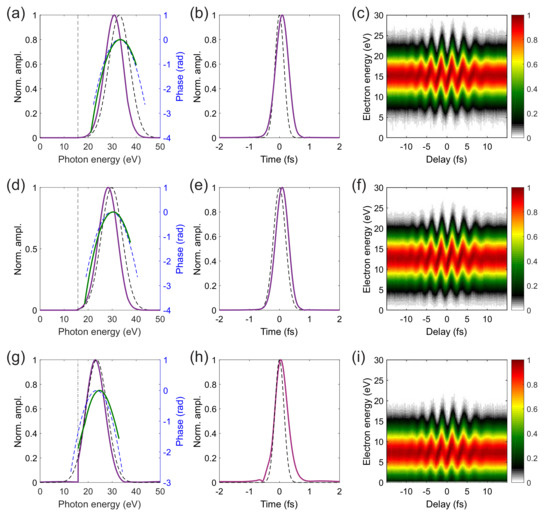
Figure 1.
Theoretical simulations. (a) Dashed lines represent the original attosecond spectral amplitude (black) and phase (blue) for a pulse with central energy corresponding to the 21st harmonic of the infrared (IR) pulse ( eV). Solid lines display amplitude (violet) and phase (green) of the corresponding calculated electron burst resulting from Ar ionization [24]. The vertical black dash-dotted line marks the position of the Ar ionization potential. (b) Temporal behaviour of the extreme-ultraviolet (XUV) attosecond pulse (black dashed) and the attosecond electron burst (solid violet). (c) Associated attosecond streaking trace. In false color it is shown the amplitude of the spectrogram . (d–i) Same quantities for a single attosecond pulse with central energy corresponding to the 19th harmonic at 29.82 eV and the 15th harmonic at 23.54 eV, respectively. The other calculations parameters are reported in the text. As a result of the atomic cross-section spectral filtering, the final photoelectron spectral amplitude bandwidths are: 8.95, 9.75, and 9.44 eV for the results in the first, second, and last row, respectively.
3. Reconstruction Results
As discussed above, the most commonly used reconstruction approaches are based on the FROG-CRAB method in combination with several reconstruction algorithms [20,29,30]. The main limitation of this approach lies in the fact that the spectrogram in Equation (1) needs to be factorized as an internal product between a pulse and gate functions, which depend only on time. To do so, we need to remove the momentum dependence from the quantum phase . This is is obtained by substituting p with the value of the electron central momentum in Equation (2). This procedure is called central momentum approximation (CMA) and allows Equation (1) to be rewritten in the form:
where the pulse function is and the gate function is , a pure phase gate. If one applies the CMA, the spectrogram in Equation (6) can be interpreted as a blind FROG trace and both pulse and gate can be retrieved with a FROG-like iterative algorithm. We underline that in a real attosecond streaking experiment FROG-like approaches are not sensitive to the actual pulse intensity as identical pulses with different peak intensities will produce the same spectrogram besides a constant multiplication factor. The attosecond pulse peak intensity can be estimated by measuring the actual XUV beam profile, the pulse energy and duration. Therefore, a precise time characterization of the attosecond pulse represents the first step towards a correct estimation of its peak intensity. Among all the proposed algorithms, the extended ptychographic iterative engine (ePIE) proved to be superior in terms of robustness, flexibility, and convergence speed [20,31]. Figure 2 shows the residual reconstruction error obtained by subtracting the simulated streaking traces displayed in Figure 1c,f,i from their reconstructions for (Figure 2a), (Figure 2b), and (Figure 2c). The first row of Figure 2 shows the residual reconstruction error obtained when ePIE is used for the reconstruction. In this case the residual error map shows a top-bottom asymmetry (negative values at high energies and positive values at low energies) which originates from the CMA at the heart of the ePIE algorithm [16]. Since the CMA is less accurate for low electron final momenta, the residual error increases upon decreasing , as clearly visible comparing Figure 2a,c. In all the ePIE reconstructions presented here, the original spectrograms of Figure 1 are down-sampled to 4096 points in energy (energy step meV) and 199 in delay (delay step fs) before reconstruction. The algorithm runs over 2000 iterations, which is more than enough to guarantee convergences after about 7 min of computational time on a common personal computer.
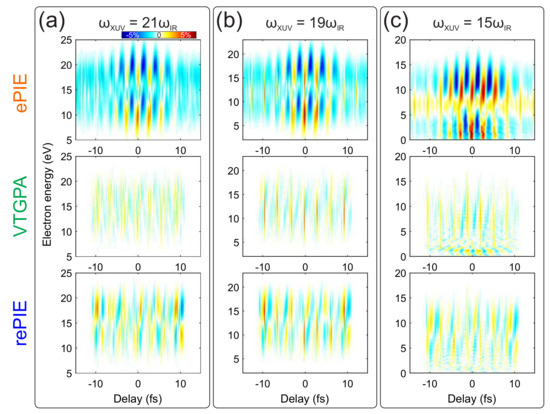
Figure 2.
(a–c) Residual error for the reconstructed spectrograms which have as input the traces in Figure 1c,f,i, respectively. The first raw, extended Ptychograpic Iterative Engine (ePIE) outputs. Second and third rows, Volkov Transform Generalized Projection Algorithm (VTGPA) and refined extended Ptychograpic Iterative Engine (rePIE) results. In all cases, VTGPA and rePIE show considerably low reconstruction error.
CMA can be avoided in FROG-CRAB reconstruction by implementing a method recently proposed by Keathley and coworkers [18], based on a a different algorithm called VTGPA. VTGPA does not use fast Fourier transformation and can handle the momentum dependence in the gate function, hence giving more accurate results. The disadvantage of this method is a notable reduction of the computational speed. The second row in Figure 2 shows the residual error obtained with VTGPA after 100 iterations. VTGPA shows a superior convergence and the final residual error is considerably smaller and does not show any systematic up-down asymmetric structure (compare first and second rows in Figure 2). Since the code is considerably slower, we were forced to strongly reduce the energy and time resolution in the VTGPA reconstruction. The simulated spectrograms are re-sampled onto 179 energy points ( meV) and 100 delay points ( fs). In these conditions the same personal computer takes 11 h to finish the 100 iterations. Our new approach attempts to combine the positive aspects of ePIE and VTGPA in order to overcome the limitations introduced by CMA at acceptable total computational times. The idea is to perform a first fast ePIE reconstruction and then “refine” the obtained result with only a few iterations of the VTGPA to correct for the error introduced by the CMA. We dubbed this method rePIE (refined extended ptychographic iterative engine). The residual errors obtained with rePIE (2000 ePIE plus 100 VTGPA iterations) for the pulses centred at , , and are shown in the third row of Figure 2. Details on the reconstructed pulses and speed convergence will be discussed in depth in the next section. Nevertheless, we can already notice that the residual spectrogram error is considerably better than the one obtained with ePIE and comparable to the VTGPA one. It is worth to notice that this is not a trivial outcome. As ePIE is based on CMA, the algorithm converges towards a solution which is the best approximation of the exact solution, but still satisfies the CMA. This point could represent a local attractor in the ensemble of the general solutions which are not based on the CMA. Therefore, there is no guarantee that the subsequent application of the VTGPA code will be able to steer the convergence away form this local minimum, towards a more general solution.
4. Comparison and Discussion
In this section we compare the results obtained with ePIE, VTGPA, and rePIE for the three attosecond pulses previously presented. We will start from the attosecond pulse centred around the 21st harmonic of the IR field for which the CMA is supposed to hold and later move towards lower photon energies.
Figure 3 shows in details the reconstructed XUV and IR pulses for ePIE (orange dots), VTGPA (green squares), and rePIE (blue open circles), in the case of attosecond pulses with spectrum centred around the 21st harmonic. The vertical dash-dotted line in Figure 3b,c shows the position of the Ar ionization potential (15.76 eV). All methods reconstruct the correct XUV pulse in time (Figure 3a), spectral amplitude (Figure 3b), and phase (Figure 3c). Also the IR pulse is reconstructed with high accuracy (Figure 3d). The error on the IR retrieval, defined as reconstructed IR electric field minus the theoretical input field, is shown in Figure 3e. VTGPA gives the best reconstruction while ePIE is characterized by the largest error. Even if this could be a limiting factor for ePIE in certain kind of experiments, like attosecond IR transient polarization spectroscopy [32], in general it represents another strength of ePIE. Indeed, the error introduced by the CMA is projected on the IR pulse and the XUV reconstruction is unaffected. Being considerably faster than VTGPA, the use of ePIE is particularly useful for attosecond metrology experiments where the CMA is a good approximation. rePIE gives slightly better IR reconstruction than ePIE, but does not reach the degree of precision of VTGPA. Nevertheless, rePIE converges much faster than VTGPA. In Figure 3f we show the behaviour of the reconstruction error for the last 100 iteration of the VTGPA code in both cases: Pure VTGPA (green) and rePIE (blue). While pure VTGPA takes around 100 iterations (roughly 11 h of computing time) to converge to an error of , after only 10 iterations (a bit more than 1 h) rePIE has already reached the convergence with an overall comparable error of .
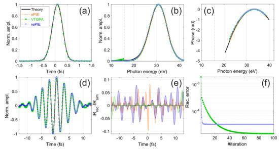
Figure 3.
Attosecond pulses with spectrum centred around the 21st harmonic. (a) Temporal amplitude profile of the XUV pulse. (b,c) Associated spectra amplitude and phase. (d) Reconstructed IR femtosecond pulse. (e) Residual error between the simulated and reconstructed IR pulse. (f) Reconstruction error of the last 100 iterations for VTGPA and rePIE algorithms as a function of iteration number. In all the figures, orange full dots represent the ePIE results, green squared marks show the VTGPA results, while the rePIE output is represented by the blue open circles.
Figure 4 shows the same quantities in the case of XUV attosecond pulses centred around the 19th harmonic. In this spectral region the CMA starts to be less accurate and for ePIE we observe very small deviations of the reconstructed spectral phase of the XUV pulse, compared to the simulations (compare green and black curve in Figure 4c). Nevertheless, the phase is properly reconstructed and the deviations are observed only at the tails of the XUV spectrum where the spectral power is small. The error on the IR pulse reconstruction is comparable to what previously found for the pulse centred around the 21st harmonic (compare orange coloured areas in Figure 3e and Figure 4e). Therefore, ePIE can still reconstruct properly the XUV pulse, even if the best IR reconstruction is achieved with VTGPA also in this case. Nevertheless, we observe that full VTGPA reconstruction starts to face a problem due to the filtering action of the atomic cross-section. The reconstructed spectral amplitude (Figure 4b) displays a second shoulder located right below the Ar ionization potential, (shown by the green shaded area in Figure 4b). This artefact probably originates from the abrupt cut of the photon spectrum at . We remark that, since the spectral phase is properly reconstructed (Figure 4c), one can remove the artefact after reconstruction, by filtering out the spectral components below and thus retrieve the perfect time envelope of the electron burst. As in the previous case, rePIE gives an outcome that lies in between the results of the two previous algorithms. The attosecond pulse is perfectly reconstructed and there is no artefact below in the spectral domain. The IR pulse residual error (Figure 4e) is smaller than the one of the previous case (Figure 3e). The stronger deviation is observed around the tails of the pulse where also the VTGPA result deviates considerably. This is probably due to the finite number of points chosen for the time axis in VTGPA. Figure 4f shows that rePIE is again considerably faster. For the full VTGPA approach convergence is reached in almost 100 iterations leading to an error of . rePIE needs only 10 additional iteration of the VTGPA to reach convergence with an error of , thus saving a great amount of computational time.
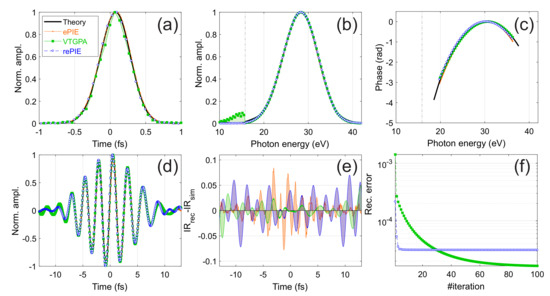
Figure 4.
Attosecond pulses with spectrum centred around the 19th harmonic. (a) Temporal amplitude profile of the XUV pulse. (b,c) Associated spectra amplitude and phase. (d) Reconstructed IR femtosecond pulse. (e) Residual error between the simulated and reconstructed IR pulse. (f) Reconstruction error of the last 100 iterations for VTGPA and rePIE algorithms as a function of iteration number. In all the figures, orange full dots represent the ePIE results, green squared marks show the VTGPA results, while the rePIE output is represented by the blue open circles.
To conclude our analysis, we study what happens when a considerable portion of the XUV spectrum lies below the target ionization potential. The results are reported in Figure 5 and show the different reconstructions for an attosecond pulse centred at the 15th harmonic. The Ar ionization potential produces a clear vertical cut in the photoelectron spectrum of Figure 5b (black solid curve). In this case the CMA is certainly not justified. Indeed, the error of the ePIE reconstruction increases when compared to the two previous cases (see Figure 2). The spectral phase in Figure 5c shows some oscillations in the region between 15 and 20 eV and it considerably deviates from the theoretical curve at high energies. The extracted chirp is −0.03 fs instead of the theoretical value of −0.02 fs. The error on the IR reconstruction (Figure 5e) is also appreciably bigger than the previous cases. Nevertheless, also in this case the majority of the reconstruction error comes from a wrongly reconstructed IR pulse and the XUV pulse is surprisingly well reconstructed also in this extreme case. A full VTGPA approach does not perform well at these energies. The artefact observed before in Figure 4b becomes stronger in this case, deeply affecting the time profile of the reconstructed electron burst. Since in this case also the reconstructed spectral phase is affected (the shaded green area in Figure 5c indicates the deviation from the theoretical input), we notice that here it will not be possible to filter out the artefact after reconstruction. Therefore, despite giving the best IR reconstruction (compare the shaded areas in Figure 5e), VTGPA will not reconstruct accurately the electron burst, especially in the energy region close to . This can be a problem for short attosecond pulses, characterized by a broad bandwidth in the VUV-XUV region [13]. Once again, rePIE brings together the positive aspects of the two algorithms. Even if it also shows an artefact below (blue area in Figure 5b), it is considerably smaller that the one obtained with full VTGPA and the spectral phase is no longer strongly affected. Compared to ePIE, rePIE reconstructed spectral phase follows more accurately the simulations also at high energies. The extracted value of the chirp is −0.0206 fs, in excellent agreement with the theoretical values. The IR residual error is also strongly reduced (blue area in Figure 5e). Finally, as shown in Figure 5f, not only rePIE is faster than full VTGPA, but also it converges to a solution characterized by a smaller residual error of instead of for full VTGPA. We recently applied rePIE to actual experimental attosecond streaking traces centered at low electron kinetic energies. The results are reported in Ref. [13] and confirm what found by the theoretical investigation here presented.
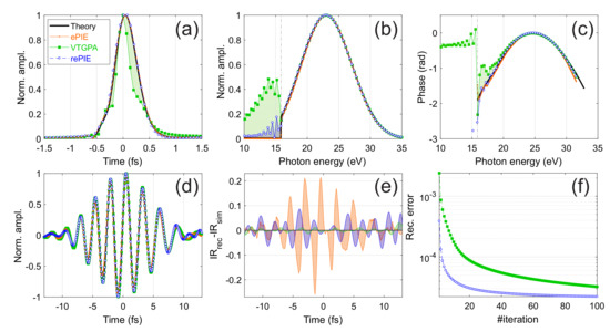
Figure 5.
Attosecond pulses with spectrum centred around the 15th harmonic. (a) Temporal amplitude profile of the XUV pulse. (b,c) Associated spectra amplitude and phase. (d) Reconstructed IR femtosecond pulse. (e) Residual error between the simulated and reconstructed IR pulse. (f) Reconstruction error of the last 100 iterations for VTGPA and rePIE algorithms as a function of iteration number. In all the figures, orange full dots represent the ePIE results, green squared marks show the VTGPA results while the rePIE output is represented by the blue open circles.
5. Conclusions
In conclusion, we showed that the CMA in FROG-CRAB reconstructions based on a ptychographic algorithm mainly affects the reconstructed IR femtosecond pulse. The lower the photoelectron kinetic energies (or XUV photon energies), the stronger the effect on both reconstructed IR and attosecond pulses. The error introduced by the CMA can be avoided if more advanced reconstruction algorithms like VTGPA are used. Nevertheless, this approach is very demanding from the point of view of computational costs and seems to suffer from numerical artefacts when the ionization potential of the target lies within the XUV spectrum. In this work, we show that an opportune combination of the two algorithms, called rePIE, can maintain their individual strengths, giving an accurate and fast reconstruction of both IR and XUV pulse. We found that this approach is particularly useful for short attosecond pulses, characterized by a broad spectrum in the VUV-XUV region.
Author Contributions
M.L. wrote the rePIE code, performed the simulations and reconstructions. All the authors participated the interpretation of the results and wrote the paper.
Funding
This research received no external funding.
Acknowledgments
The authors wish to thank P. D. Keathley and L. Pedrelli for their help in implementing the VTGPA code.
Conflicts of Interest
The authors declare no conflict of interest.
Abbreviations
The following abbreviations are used in this manuscript:
| XUV | extreme-ultraviolet |
| VUV | vacuum-ultraviolet |
| IR | infrared |
| CMA | central momentum approximation |
| FROG-CRAB | Frequency Resolved Optical Gating for the Complete Reconstruction of Attosecond Bursts |
| ePIE | extended Ptychograpic Iterative Engine |
| VTGPA | Volkov Transform Generalized Projection Algorithm |
| rePIE | refined extended Ptychograpic Iterative Engine |
References
- Zewail, A.H. Femtochemistry: Atomic-Scale Dynamics of the Chemical Bond. J. Phys. Chem. A 2000, 104, 5660–5694. [Google Scholar] [CrossRef]
- Krausz, F.; Ivanov, M. Attosecond physics. Rev. Mod. Phys. 2009, 81, 163–234. [Google Scholar] [CrossRef]
- Nisoli, M.; Decleva, P.; Calegari, F.; Palacios, A.; Martín, F. Attosecond Electron Dynamics in Molecules. Chem. Rev. 2017, 117, 10760–10825. [Google Scholar] [CrossRef] [PubMed]
- Itatani, J.; Quéré, F.; Yudin, G.L.; Ivanov, M.Y.; Krausz, F.; Corkum, P.B. Attosecond Streak Camera. Phys. Rev. Lett. 2002, 88, 173903. [Google Scholar] [CrossRef] [PubMed]
- Drescher, M.; Hentschel, M.; Kienberger, R.; Uiberacker, M.; Yakovlev, V.; Scrinzi, A.; Westerwalbesloh, T.; Kleineberg, U.; Heinzmann, U.; Krausz, F. Time-resolved atomic inner-shell spectroscopy. Nature 2002, 419, 803–807. [Google Scholar] [CrossRef]
- Schultze, M.; Fieß, M.; Karpowicz, N.; Gagnon, J.; Korbman, M.; Hofstetter, M.; Neppl, S.; Cavalieri, A.L.; Komninos, Y.; Mercouris, T.; et al. Delay in Photoemission. Science 2010, 328, 1658–1662. [Google Scholar] [CrossRef]
- Sabbar, M.; Heuser, S.; Boge, R.; Lucchini, M.; Carette, T.; Lindroth, E.; Gallmann, L.; Cirelli, C.; Keller, U. Resonance Effects in Photoemission Time Delays. Phys. Rev. Lett. 2015, 115, 133001. [Google Scholar] [CrossRef]
- Cavalieri, A.; Muller, N.; Uphues, T.; Yakovlev, V.; Baltuska, A.; Horvath, B.; Schmidt, B.; Blumel, L.; Holzwarth, R.; Hendel, S.; et al. Attosecond spectroscopy in condensed matter. Nature 2007, 449, 1029–1032. [Google Scholar] [CrossRef]
- Neppl, S.; Ernstorfer, R.; Cavalieri, A.L.; Lemmel, C.; Watcher, G.; Magerl, E.; Bothschafter, E.M.; Jobst, M.; Hofstetter, M.; Kleineberg, U.; et al. Direct observation of electron propagation and dielecric screening on the atomic length scale. Nature 2015, 517, 342–346. [Google Scholar] [CrossRef]
- Siek, F.; Neb, S.; Bartz, P.; Hensen, M.; Strüber, C.; Fiechter, S.; Torrent-Sucarrat, M.; Silkin, V.M.; Krasovskii, E.E.; Kabachnik, N.M.; et al. Angular momentum-induced delays in solid-state photoemission enhanced by intra-atomic interactions. Science 2017, 357, 1274–1277. [Google Scholar] [CrossRef]
- Ossiander, M.; Riemensberger, J.; Neppl, S.; Mittermair, M.; Schäffer, M.; Duensing, A.; Wagner, M.S.; Heider, R.; Wurzer, M.; Gerl, M.; et al. Absolute timing of the photoelectric effect. Nature 2018, 561, 374–377. [Google Scholar] [CrossRef] [PubMed]
- Chini, M.; Gilbertson, S.; Khan, S.D.; Chang, Z. Characterizing ultrabroadband attosecond lasers. Opt. Express 2010, 18, 13006–13016. [Google Scholar] [CrossRef] [PubMed]
- Pedatzur, O.; Trabattoni, A.; Leshem, B.; Shalmoni, H.; Castrovilli, M.C.; Galli, M.; Lucchini, M.; Månsson, E.; Frassetto, F.; Poletto, L.; et al. Double Blind Holography of Attosecond Pulses. Nat. Photonics. in press.
- Mairesse, Y.; Quéré, F. Frequency-resolved optical gating for complete reconstruction of attosecond bursts. Phys. Rev. A 2005, 71, 011401. [Google Scholar] [CrossRef]
- Wei, H.; Morishita, T.; Lin, C.D. Critical evaluation of attosecond time delays retrieved from photoelectron streaking measurements. Phys. Rev. A 2016, 93, 053412. [Google Scholar] [CrossRef]
- Cattaneo, L.; Vos, J.; Lucchini, M.; Gallmann, L.; Cirelli, C.; Keller, U. Comparison of attosecond streaking and RABBITT. Opt. Express 2016, 24, 29060–29076. [Google Scholar] [CrossRef] [PubMed]
- Cirelli, C.; Sabbar, M.; Heuser, S.; Boge, R.; Lucchini, M.; Gallmann, L.; Keller, U. Energy-Dependent Photoemission Time Delays of Noble Gas Atoms Using Coincidence Attosecond Streaking. IEEE J. Sel. Top. Quantum Electron. 2015, 21, 1–7. [Google Scholar] [CrossRef]
- Keathley, P.D.; Bhardwaj, S.; Moses, J.; Laurent, G.; Kärtner, F.X. Volkov transform generalized projection algorithm for attosecond pulse characterization. New J. Phys. 2016, 18, 073009. [Google Scholar] [CrossRef]
- Gaumnitz, T.; Jain, A.; Wörner, H.J. Complete reconstruction of ultra-broadband isolated attosecond pulses including partial averaging over the angular distribution. Opt. Express 2018, 26, 14719–14740. [Google Scholar] [CrossRef]
- Lucchini, M.; Brügmann, M.; Ludwig, A.; Gallmann, L.; Keller, U.; Feurer, T. Ptychographic reconstruction of attosecond pulses. Opt. Express 2015, 23, 29502–29513. [Google Scholar] [CrossRef] [PubMed]
- Kitzler, M.; Milosevic, N.; Scrinzi, A.; Krausz, F.; Brabec, T. Quantum theory of attosecond XUV pulse measurement by laser dressed photoionization. Phys. Rev. Lett. 2002, 88, 173904. [Google Scholar] [CrossRef] [PubMed]
- Wigner, E.P. Lower limit for the energy derivative of the scattering phase shift. Phys. Rev. 1955, 98, 145–147. [Google Scholar] [CrossRef]
- Dahlström, J.M.; L’Huillier, A.; Maquet, A. Introduction to attosecond delays in photoionization. J. Phys. B At. Mol. Opt. Phys. 2012, 45, 183001. [Google Scholar] [CrossRef]
- West, J.B.; Marr, G.V. The absolute photoionization cross sections of helium, neon, argon and krypton in the extreme vacuum ultraviolet region of the spectrum. Proc. R. Soc. Lond. A 1976, 349, 397–421. [Google Scholar] [CrossRef]
- Mauritsson, J.; Johnsson, P.; Gustafsson, E.; L’Huillier, A.; Schafer, K.J.; Gaarde, M.B. Attosecond Pulse Trains Generated Using Two Color Laser Fields. Phys. Rev. Lett. 2006, 97, 013001. [Google Scholar] [CrossRef]
- Ossiander, M.; Siegrist, F.; Shirvanyan, V.; Pazourek, R.; Sommer, A.; Latka, T.; Guggenmos, A.; Nagele, S.; Feist, J.; Burgdörfer, J.; et al. Attosecond correlation dynamics. Nat. Phys. 2016, 13, 280–285. [Google Scholar] [CrossRef]
- Isinger, M.; Squibb, R.; Busto, D.; Zhong, S.; Harth, A.; Kroon, D.; Nandi, S.; Arnold, C.L.; Miranda, M.; Dahlström, J.M.; et al. Photoionization in the time and frequency domain. Science 2017, 358, 893–896. [Google Scholar] [CrossRef]
- Vos, J.; Cattaneo, L.; Patchkovskii, S.; Zimmermann, T.; Cirelli, C.; Lucchini, M.; Kheifets, A.; Landsman, A.S.; Keller, U. Orientation-dependent stereo Wigner time delay and electron localization in a small molecule. Science 2018, 360, 1326–1330. [Google Scholar] [CrossRef]
- Kane, D. Recent progress toward real-time measurement of ultrashort laser pulses. IEEE J. Quantum Electron. 1999, 35, 421–431. [Google Scholar] [CrossRef]
- Gagnon, J.; Goulielmakis, E.; Yakovlev, V. The accurate FROG characterization of attosecond pulses from streaking measurements. Appl. Phys. B 2008, 92, 25–32. [Google Scholar] [CrossRef]
- Lucchini, M.; Lucarelli, G.D.; Murari, M.; Trabattoni, A.; Fabris, N.; Frassetto, F.; Silvestri, S.D.; Poletto, L.; Nisoli, M. Few-femtosecond extreme-ultraviolet pulses fully reconstructed by a ptychographic technique. Opt. Express 2018, 26, 6771–6784. [Google Scholar] [CrossRef] [PubMed]
- Sommer, A.; Bothschafter, E.M.; Sato, S.A.; Jakubeit, C.; Latka, T.; Razskazovskaya, O.; Fattahi, H.; Jobst, M.; Schweinberger, W.; Shirvanyan, V.; et al. Attosecond nonlinear polarization and light-matter energy transfer in solids. Nature 2016, 534, 86–90. [Google Scholar] [CrossRef] [PubMed]


© 2018 by the authors. Licensee MDPI, Basel, Switzerland. This article is an open access article distributed under the terms and conditions of the Creative Commons Attribution (CC BY) license (http://creativecommons.org/licenses/by/4.0/).