Featured Application
The proposed circuit model is able to foresee the overall current distortion of different lamp configurations. This feature is very useful in the optimal design of lighting systems when a key target is the mitigation of the current distortion due to the power converter inside the energy-saving lamps.
Abstract
Energy-saving lamps are equipped with converters enabling high energy efficiency at the cost of injecting very distorted currents on the mains. The problem is more complex in the emerging smart-lighting scenario where these lamps are also used to perform additional tasks. Harmonics mitigation at the lamp level is expensive; consequently, an optimal lighting system design aiming at reducing both costs and current distortion of the whole lighting system is necessary. A tool able to emulate the current drawn from the lamps is necessary for optimal design. Such a tool has also to consider the fluctuations of the voltage on the mains that usually occur throughout the day. In this perspective, a parametric PSpice circuit is proposed and the netlist is reported in this work. Moreover, the simple procedure to be adopted for computing the parameters is also described. The validation has confirmed the ability of the proposed circuit in emulating the current drawn from various CFLs and LED lamps under different supplying voltage.
1. Introduction
Energy efficiency is a crucial target in view of a sustainable energy future [1], thus, different policies to improve energy efficiency have been internationally introduced [2,3,4,5,6]. European Council has initially set the target of 27% (that should become 30%) energy savings by 2030. Moreover, the European Union is pushing towards “nearly zero-energy buildings” by introducing legal requirement in the construction of new buildings [7]. In this perspective, the European Union has also decided to phase out inefficient light bulbs and, similarly, in the U.S.A., the manufacture of light bulbs that do not meet federal energy-efficiency standards is prohibited according to the Energy Independence and Security Act [8,9].
Energy-saving lamps (ESLs) are consequently the natural choice for lighting system retrofitting as well as for designing future lighting systems. An ESL is a non-linear load due to the converters adopted in the lamp that draws a very distorted current from the mains. In the Smart Lighting scenario, intelligent lamps present new capabilities and functionality (e.g., continuously flashing to signal an intrusion, use sensors for automatic dimming, and so on) making them more than simple illumination systems [10]. Such additional tasks involve driving algorithms for the converters that may intensify the harmonic distortion. Obviously, the effect of the current drawn from a single lamp is negligible. On the other hand, the effect of the total current harmonics injected on the mains cannot be neglected in large lighting systems in view of the widespread use of ESLs in building and streets. The harmonics negatively affect the power network: reduction of the cable ampacity and life, while the losses and EMI issues increase [11]; premature aging and failures of capacitor banks used for power factor correction and ancillary services [12,13,14,15]; undesired losses in motors and transformers windings with related life expectancy reduction [16,17]. The large use of ESLs will involve additional issues on future smart grids that use network control and management techniques based on measurements that may be affected by the harmonics [18]. The problem is exacerbated by the ESLs since dealing with the large distorted current due to a very great number of dispersed ESLs is more complex than in case of a single large harmonics source [19]. Therefore, there is a noteworthy need for mitigation of the harmonics due to ESL based lighting systems. The addition of filters, power factor corrector circuits, and other devices in the ESL increase the lamp cost and consequently the economic investment for both retrofitting and new lighting systems [20,21,22,23,24]. On the other hand, although a single compensation circuit for the whole lighting system may be less expensive [25], it has to be revised each time a new lighting system retrofit is performed.
The best choice from cost and flexibility point of view is the harmonic mitigation at lighting system design stage. The optimal lighting system design aiming at mitigation of the distorted current drawn from the whole lighting system requires a tool for estimating such a current when different lamps configurations are adopted (number, type, nominal parameter, and so on). In such a case the best configuration is the one with the greatest harmonic cancellation and lowest THD [25,26,27,28,29].
The proposed parametric PSpice circuit is suitable to perform this task. More specifically, the current drawn from a given ESL under a variable voltage on the main is emulated by means of a generalized PSpice netlist with parametric components. The parameters of an ESL can be obtained by few simple current measurements to be performed at the lamp terminals. These parameters are the coefficients of the functions obtained by linear interpolation of the rms of the current harmonics. In view of the increasing attention in the reduction of harmonic injection, the coefficient of these polynomial functions should be provided by manufactures in the ESL datasheet in the future, regardless the specific use of that information in this paper.
The PSpice circuit validation has been performed comparing the measured and simulated currents: the results have confirmed the suitability of the model. The circuit can be used to predict the current waveform of each lamp and, consequently, the overall current drawn from the lighting system for different configurations can be foresee. Therefore, it is a useful tool for the optimal design of a new lighting system or its subsequent optimal retrofit.
2. Related Works
The design of the lighting system plays a fundamental role because it is a prime component to help to living and feeling better in the private houses, in the offices and industrial locations. In these terms, the design should take into account the light level and the uniformity of the light pattern, the aesthetic appearance, the economic benefit, the safety and appropriate equipment [30]. Safety issues should be more cared in some industrial applications and in street lighting. Only ESLs will be used in future smart lighting systems, then there is an increasing interest in studying the new devices in their large applications.
The optimal lighting system design in different indoor applications of ESLs have been investigated by considering several constraints and objectives: cost saving, energy efficiency and management, functional suitability, system integration, people satisfaction, and quality of lighting [31,32,33,34,35,36,37,38]. Moreover, it is important to point out the different innovative solutions in the modern agriculture consist on the development of facilities LED lighting technology. Among the different advantages, it can be realized a continuous production of crops and, consequently, the growth factors (temperature, light, etc.) can be controlled during the whole process while it is also reduced the use of pesticide [39,40,41,42]. It is evident that the use of parallel optimization algorithms [43] plays a key role in the optimal design of the lighting system that requires investment and operating costs minimization, as well as uniform light distribution over the plant growing area, accounting for light intensity capability and shading effects [44,45]. In outdoor applications, accurate methods have been developed to test the road lighting effects to ensure a good visibility in the street [46,47,48,49,50].
Although several key aspects of the optimal lighting system design have been considered until now, the power quality degradation due to the employment of the ESLs has been neglected in both indoor and outdoor lighting design. In the perspective of an optimal and efficient design, the distorted current drawn by a large number of lamps have to be considered. The parametric PSpice circuit proposed in this paper enables to consider power quality degradation at the planning stage of the lighting system and, consequently, overcome the aforesaid limitation of previous works on the optimal lighting design.
The impact on the grid of the current harmonics produced by the CFLs and LED lamps has been analysed in depth so far [51,52,53,54,55,56,57,58]. In [51] the results of the experimental evaluation of electrical characteristics of several LED lamps from different manufacturers have been reported. The behaviour of each lamp using different supply voltage has been considered and the amount of current harmonic injected into the grid has been measured. The main goal of [52] has been the comparison of different house hold illumination appliances and the monitoring of the power quality degradation. In [53] the current harmonics that are injected into the utility-grid by the different types of LED lamps that are available in the Indian market have been considered and the results have been compared with the IEC 61000-3-2 guidelines. In [54] a comparison between the use of incandescent lamps and ESLs has been carried out for a large building. In [55] the measurements in two private houses and on low voltage side of the distribution transformer supplying these houses have been performed. Additionally, in this case the incandescent lamps have been replaced with the energy saving ones. It is worth highlighting that in [56] the impact of the current harmonic due to by several domestic appliances, together with many LED lamps has been analysed. It is also interesting to note how the power quality issues in term of harmonics generated by lighting system when both CFLs and LED lamps are employed have been studied [57]. In such a work the design of a filter circuit for harmonic reduction in lighting system applications has been considered. Different LED light bulbs have been compared in [58], focusing on the current harmonic emission and, consequently, on the negative impact on the distribution grid. In [59], a method to examine the effect on harmonic distortion levels in the distribution network through a custom software has been proposed. Although the current distortion has been investigated in these works, there were not developed any model able in predicting the distorted current. Although the harmonics due to the ESLs have been studied in these works, they do not provide any method to esteem the harmonic distortion due to them.
Several works have treated the prediction of the amount of current harmonic that the ESLs inject into the power grid [60,61,62,63,64,65,66,67,68,69,70,71,72]. In [60] has been investigated the effect of the employing of many energy-saving lamps on the power grid in New Zeeland. A Norton equivalent has been used to emulate a large number of houses assumed as series of distributed loads. The main objective of [61] has been the prediction of the maximum number of CFLs that can be used without overcome a threshold value of THD imposed by the users. In [62] the results of a research performed on energy-efficient electronic ballasts for T8 fluorescent lamps have been presented. Unlike the previous cases, the CFL behaviour in a distribution system a fixed harmonic injection method has been adopted, where the single CFL has been modelled by means of an ideal current source. In this way, a possible solution developed in the PSCAD/EMTDC environment to model the CFL ballast circuit has been proposed in [63]. The solution analysed the interactions of several CFLs connected to an electrical network at the same time. It has been studied the error between the measured current waveform and the ones obtained through the fixed harmonic current injection. Moreover, the tensor analysis with phase dependency is used with the aims to take into account the harmonic interaction of the mains voltage in the CFL harmonic currents. The analysis of the power factor and harmonic emission of CFLs have highlighted that the current drawn of the lamps are influenced by the main voltage variation [60,61,62,63]. Consequently, when multiple CFLs interact together through the AC system impedance, the harmonic current injection method is not always accurate. In [64], the black box CFL behaviour is obtained analysing the current waveform drawn as a function of the main voltage applied. The current has been modelled by a mathematical function given by the difference between two exponentials. Even if many results have been accurate, some particular CFLs under test have had to use some ad hoc adjustment to fit accurately with the measurements.
Some researchers have worked out the behaviour of the CFL using an equivalent electrical circuit [65,66,67,68,69,70,71,72]. A common and general model is depicted in Figure 1, where the key circuit components are: a diode bridge that rectifies the main voltage, an AC equivalent resistor (Rac) and a DC smoothing electrolytic capacitor (C) supplying the downstream inverter that, in turn, feeds the fluorescent tube. Both the inverter and the fluorescent tube can be modelled as a unique equivalent resistance, RD, since they behaviour like to a constant load for the DC busbar. In [65,66] an admittance model that depends on some internal parameters (firing and extinction angles) that, in turn, depend on the voltage waveform being used instead of the general model. A method based on the measurements to obtain harmonic models of power electronic-based home appliances, among which ESLs, has been presented in [65]. In [66] a model based on harmonically coupled admittance matrix used to study harmonics in static converters of ESLs have been proposed. However, admittance model it is valid only in a specific condition of the supply voltage. In [67] a simplified version of the general model is adopted where the AC resistor has been neglected since it presents a small resistance. However, this approximation may lead to non-realizable infinite slopes of the AC current rising edge.

Figure 1.
Simple equivalent circuit usually adopted in literature for modelling a CFL [67,68,69,70,71,72].
Similarly, the CFL equivalent circuit considering the AC resistance has been proposed in [68]. The model considers that the behaviour of the CFL electrical circuit is similar to the one shown in Figure 1. The supply voltage has been modelled with the series of the fundamental and inter-harmonic voltage generators with their network equivalent impedance. In [69] the CFL parameter estimation has been obtained as a detailed analysis of the electrical model developed in [68], where the former used a non-linear least-square procedures based on actual measurements. The resolution is based on the Newton method calculating the terms of the Jacobian matrix by finite difference approach. The study of CFL impact and the related model has involved the determination of the CFL equivalent circuit parameters Rac, C, and RD described previously. It is worth noting that in literature several procedures are developed to determine the parameters from the supply voltage and AC current measurements [68,69]. Other studies deal with the estimation of other non-linear loads using least-square algorithms [70,71,72]. In [70,71] the parameter estimation of single-phase rectifiers by analysing several non-linear sets of equations has been performed. More specifically, the former has proposed the two methods to esteem the electrical components in the input rectifier that there are in many electronic equipment available in the market. The latter has presented an estimation algorithm based on a rectifier model and actual measurements. A methodology for the estimation of the main parameters related to the harmonic due industrial loads has been considered in [72] where aggregated measurements of the total load has been performed Regarding the LED light bulb, few works investigate the electrical model for the current drawn [73].
The procedures described before offers several rules that enable to obtain the circuit model of CFLs available on the market, but they require the knowledge of the ballast internal circuit components and not negligible computational resources, which make them unsuitable tool for optimal lighting system design. Moreover, the circuit model includes non-linear components. On the other hand, as said before, although several objective and constraints have been considered so far in the optimal lighting system design, the harmonic mitigation target has been totally neglected. Therefore, a parametric PSpice circuit overcoming these limitations has been proposed in the following. The knowledge of the ballast circuit, driver, package, and so on, is not necessary to obtain the parameters to be used in the proposed PSpice circuit. Indeed, any ESL can be treated as a black box, and the components of the circuit are simply obtained with some electrical measurements, that is, the amplitude and phase shift of the fundamental current and harmonics drawn by the ESL. An additional advantage of the proposed circuit is that it contains only linear components and the circuit simulation is very fast and it requires little computational effort.
3. Materials and Methods
The measurements of the current drawn from several ESLs from different manufactures have confirmed the presence of odd harmonics while even harmonics, subharmonics, and inter-harmonics are almost negligible. Moreover, the measurements have also confirmed a low voltage total-harmonic-distortion, which is less than 4%. Therefore, in the following the key equations of non-sinusoidal periodical instantaneous electric quantities in the absence of subharmonics and inter-harmonics are discussed. After that, the test rig and the measurements are presented with the proposed parametric PSpice circuit able in emulating the current drawn by the lamps under variable voltage on the mains.
3.1. Non-Sinusoidal Periodical Electric Quantities
Considering a circuit operating at steady-state conditions, the non-sinusoidal periodical instantaneous electric quantities, that is the voltage v(t) and the current i(t), can be represented by means of the Fourier series in the absence of subharmonics and inter-harmonics [74]:
Key terms are the power system fundamental frequency of the voltage, v1(t), and current, i1(t) [74]:
Grouping the constant term with the harmonics [74]:
any non-sinusoidal periodical instantaneous electric quantity can be summarized according the IEEE Std-1459TM [74]:
Without loss of generality, it can be set:
and also . Therefore:
The instantaneous power related to the fundamental frequency deriving from these equations is:
and the fundamental apparent power, S1, is then obtained from the fundamental active power, P1, and the fundamental reactive power, Q1, through the following equation [74]:
that, in turn, is part of the overall apparent power, S, that includes the harmonics contribution (that is the non-fundamental apparent power) [74]:
where the current distortion power, DI, the voltage distortion power, DV, and the harmonic apparent power, SH, are obtained from the evaluation of the rms value of vH(t), that is VH, and iH(t), that is IH [74]:
The harmonics related to the voltage on the mains are negligible in comparison with the current harmonics, and it is also confirmed by the measurements. Consequently, the term vH(t) in Equation (4) can be neglected, and then the apparent power is approximated to:
Therefore, modelling the current harmonics enables to estimate the non-active powers Q1 and DI that involve undesired power losses in the line. It is worth noting that, while the current harmonics pertain to the undesired term DI, the fundamental current affect the active power as well as the useless power Q1. Therefore, it is useful to consider the fundamental current divided into two components [75,76]:
It is easy to prove that:
Therefore, the term iP1(t) affects only the active power, then in the following it is called “active current”. The term iQ1(t), affects only the reactive power, then in the following it is called “reactive current”. Finally, as expected, in all performed tests for all the lamps, the phase shift of the fundamental frequency current drawn was always: (with respect to the voltage on the mains), which implies a positive value of in Equation (12).
3.2. Test Rig
The measurements of the amplitude and phase shift of the fundamental and harmonic currents have to be performed in order to obtain the components of the proposed PSpice circuit. For a given ESL, these measurements have to be performed by setting five voltage levels at the lamp terminals: 0.9 Vnom, 0.95 Vnom, Vnom, 1.05 Vnom, and 1.1 Vnom. For each current harmonic, a polynomial function has to be obtained by measurements interpolation. Similarly, polynomial functions have to be obtained for, respectively, the active and reactive current. The coefficients of these polynomial functions have to be used to select the components of the PSpice circuit according the rules that are described in the next section. Moreover, the quantities related to these components are also related to these coefficients as described in the following. With this in mind, this section describes the test rig used to set the desired voltage levels across the lamp terminals and to perform the aforesaid measurements.
Figure 2 and Figure 3 depict the measurements of the fundamental current and the odd current harmonic amplitudes up to the 13th for both a CFL and a LED light bulb. The measurements highlighted that a linear interpolation of the current harmonics turns out to be enough accurate:
with K the number of harmonics considered for emulating the waveform of the current drawn from the lamp.
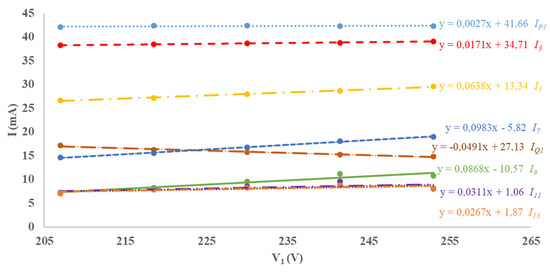
Figure 2.
Measured amplitude of the fundamental current and greatest harmonics for a CFL. The linear interpolation functions are reported on the right with the related current symbol.
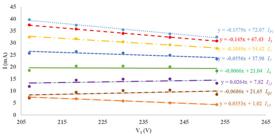
Figure 3.
Measured amplitude of the fundamental current and greatest harmonics for a LED. The linear interpolation functions are reported on the right with the related current symbol.
Remark 1.
is always positive regardless its trend in Equation (14) because it is obtained by multiplying I1 with , where the former is positive by definition while the latter has been previously proved to be positive . Similar considerations are valid for as well as for the terms in the related interpolation functions. On the other hand, although I1 is positive by definition, may be positive or negative, it depends on .
Remark 2.
Considering the previous remark and that V1 is positive by definition, at least one between
and in the interpolation function have to be positive. Similar considerations are always valid for and , while for and are valid only when is positive. On the other hand, when is negative, a dual behaviour occurs, that is at least one between and in the interpolation function have to be negative.
In the test rig (Figure 4), a transformer with continuous variable transform ratio (variac) is connected to the mains voltage with the aim of emulating the variable voltage on the mains. In other words, each time a measurement has to be performed at a given voltage level, the variac is properly tuned to emulate such a voltage level across the lamp terminals. The variac feeds the ESL through a power analyser used to measure the voltage across the lamp terminals as well as to measure the fundamental and harmonic currents (in terms of amplitude and phase shift) drawn. Moreover, to simultaneously observe the current harmonics amplitude and the waveforms of the voltage and current at ESL terminals, an oscilloscope is also used. More specifically, the current drawn from the ESL has been displayed through the oscilloscope. The power analyser has a 1 A shunt probe that offers a high resolution and accuracy for testing currents as low as 80 μA. This enables the meter to measure standby power as low as 20 mW at 240 V. The maximum voltage peak can reach 2kV, with an accuracy of 20 mV. The power analyser has a bandwidth of 1 MHz.

Figure 4.
Experimental setup. A variac, connected to the mains, feeds the ESL through a power analyser that acquires the measurements. The oscilloscope displays the waveforms.
The measurements have been performed in the range of ±10% of the rated voltage due to the voltage variations that is allowed for the utility [77]. Throughout the day, the rated voltage could suffer of some variations due to the distributed renewable generators into the network, the load variations, the network configurations and so on, without the possibility for the users to do anything about it [78].
Figure 5 shows the amplitude of the current harmonics normalized with respect to the fundamental one, in case of a CFL with 212V (rms) at its terminals. The normalized harmonic amplitudes, in blue, are sorted in ascending order and the abscissa reports the related harmonic. The figure also reports, in red, the THD error in percentage when some current harmonics are neglected, assuming as THD reference, THDI,TOT, the one computed considering the harmonics until the 50th. More specifically, for a given harmonic, n, the THD error, , is obtained when a set of m harmonics are neglected. Harmonic n and those on its left in the figure belong to this set. The current THD reference is [74]:
while the THD referred to a given current harmonic n, THDI,n, is computed subtracting the aforesaid m current harmonic amplitudes:
with an array where the amplitudes of the current harmonics have been ascending sorted and p indicates the position in the sequence. Consequentially the percentage error referred to the THDI,n is equal to:

Figure 5.
Normalized current harmonics and THD error, when the CFL is feed with 212 V.
In the THD error diagram, the first red point on the left has been calculated by removing from the total current the harmonic that has the smallest amplitude (that is the 50th), the second point is calculated neglecting the two smallest current amplitude (that is the 50th and 48th) and so on, until it is removed the 3rd current harmonic.
As can be seen from the Figure 5, for the CFL under test when the supplying voltage is 212 V, the THD percentage error is less to 1% by removing the smallest m = 38 (that is n = 23) current harmonics amplitudes (that is, considering only the 3rd, 5th, 7th, 9th, 11th, 13th, 15th, 17th, 19th, 21th, and 27th harmonics). On the other hand, by removing m = 46 harmonics, n = 9 (considering only the 3rd, 5th, and 7th), the percentage error is less than 10%. Figure 6 shows the same quantities when the voltage is 237 V.

Figure 6.
Normalized current harmonics and THD error, when the CFL is feed with 237 V.
A similar reasoning is valid for a LED lamp under test. Figure 7 depicts the normalized current harmonics and the THD percentage error. It is less to 1% by removing the smallest m = 41 (that is n = 15) current harmonics (that is, considering only the 3rd, 5th, 7th, 9th, 11th, 13th, 17th, and 19th harmonics). On the other hand, by removing m = 46 harmonics, n = 9 (considering only the 3rd, 5th, and 7th), the percentage error is less than 10%. Figure 8 reports the quantities for the LED when the voltage is 237 V.
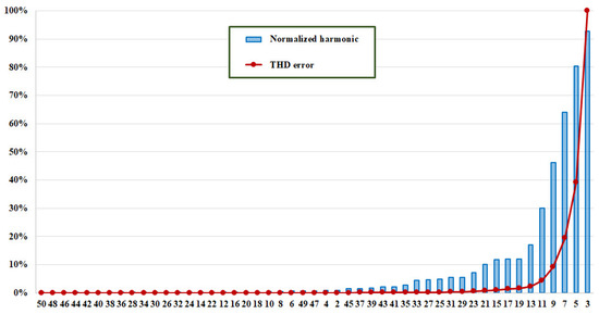
Figure 7.
Normalized current harmonics and THD error, when the LED light bulb is feed with 212 V.

Figure 8.
Normalized current harmonics and THD error, when the LED light bulb is feed with 237 V.
3.3. PSpice Model for Emulating the Current Drawn from an ESL
The proposed circuit model accounts for the change of the current drawn from a lamp when the rms voltage, V1, on the mains varies within the range allowed by the regulation (±10% of Vnom). More specifically, the model emulates the variation of the value of the rms, I1, and the change in the phase shift, , of the fundamental frequency current, i1(t). The model also emulates the variation of the rms of any other current harmonic, Ik, while it neglects any variation of the phase offset, (that is the phase offset at nominal voltage is considered). A graphical representation of the proposed circuit that accounts for the previous interpolation functions is reported in Figure 9.

Figure 9.
Proposed linear equivalent circuit of a generic ESL.
The components in the subcircuits called “Active”, “Reactive”, and “kth harmonic” emulate the behaviour of, respectively, , , and in Equation (14). According the circuit model in the figure and the equations in (14), the following equations are valid:
Then accounts for the constant term , accounts for the linear term and so on:
In the previous equations, the currents , and are independent from V1 since they arise from the constant terms in (14). Therefore, their waveforms are emulated by means of independent current generators in the equivalent circuit (Figure 9).
It is useful to recall that, when a constant term is negative (for example ) the related generator ( in such an example) is in antiphase with the overall current it belongs to ( in such an example). Consequently, according to Remark 2, the other term ( in such an example) is definitively positive because the related current ( in such an example) has to be in phase with the overall current. Moreover, the amplitude of the “in-phase” current () is greater than the amplitude of the “antiphase” current () according to Remark 1.
The voltage independent generator, vFk, with an element in series are responsible for emulating the current . The voltage independent generator has an angular frequency k times greater than the mains voltage and the same amplitude:
where is the phase offset of the kth harmonic current according to Equation (6); d can assume only two values +1 or −1, it depends on the component selected by the switches.
When the circuit component adopted is an inductor then d = 1, otherwise, when it is chosen a capacitor d = −1. It is worth noting that this voltage generator does not emulate the kth voltage harmonic on the mains but it is a fictitious generator belonging to the lamp model.
By using superposition theorem, it can be noted that such a fictitious voltage independent generator supplies only the aforesaid component, e.g., the inductor when d = 1 (see Figure 10). Therefore, at steady-state, when an inductor Lk is adopted the steady-state current trough it due to vFk is:
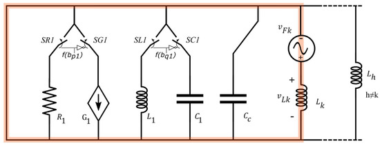
Figure 10.
Equivalent circuit when only vFk works while the other independent generators are turned off. It is apparent that this generator supplies only Lk.
When is positive, the phase of is and the previous equation becomes:
that is presents the same phase of . These currents can present also the same amplitude by properly choosing Lk:
When is negative, the phase of is since this current is in antiphase with , moreover Equation (21) becomes:
Once again presents the same phase offset of thanks to the adopted waveform of the fictitious voltage generator. These currents can present also the same amplitude by properly choosing Lk:
Therefore, by using a fictitious voltage generator with the waveform reported in Equation (20) and an inductor is always possible emulate the linear term bk:
When bk is equal to 0, the amplitude of Ik is independent from the voltage on the mains, then only the independent current generator is considered while the fictitious independent voltage generator and the inductor are removed.
When a capacitor Ck is adopted (then d = −1) the steady-state current trough it due to vFk is:
When is positive the previous equation becomes:
that is, presents the same phase of like to the previous case where an inductor has been considered. These currents can present also the same amplitude by properly choosing Ck:
and, more in general, it is always possible to emulate the linear term bk also using the fictitious voltage from Equation (20) and a capacitor:
In [75] and [76] have been presented, respectively, a circuit model (called “fundamental current circuit”, Figure 9) of the active and reactive current as well as the related PSpice model. The model of the fundamental current has been slightly modified in this work and for sake of completeness the main considerations and relations are reported in the following.
The active current has to be in phase with the mains voltage since the lamp is a load. Notwithstanding, when the constant term, aP1, is negative the independent current generator is in antiphase with the mains voltage. On the other hand, in such a case, the term bP1 has to be positive according to Remark 2, that is the current ibP1 must be in phase with the mains voltage. Moreover, its amplitude has to exceed the other in the voltage range of application (±10% of Vnom). Similarly, when the linear term, bP1, is negative the current ibP1 is in antiphase with the mains voltage, but the term aP1 is positive (according to Remark 2) and enough to ensure that the overall active current is in phase with the mains voltage in the range of application of the model. It is worth noting that negative values of bP1 highlights a reduction of the active current drawn from the lamp as the mains voltage increases. Therefore, in the PSpice circuit a resistor is adopted when ibP1 is positive (to emulate an increasing current in phase with the mains voltage), otherwise a voltage controlled current source (VCCS), G1, is considered:
Finally, no issues arise when both terms are positive. In such a case the independent generator is in phase with the mains voltage and a resistor is adopted to emulate the increasing active current drawn by the lamp as the voltage on the mains increases.
When IQ1 is positive, the reactive current leads the mains voltage. In such a case, if the constant term, aQ1, is negative then the related independent current generator lags the mains voltage. Therefore, the term bQ1 has to be positive (according to Remark 2), that is the current ibQ1 must lead the mains voltage. Moreover, its amplitude has to exceed the other in the voltage range of application (±10% of Vnom). Similarly, when the linear term, bQ1, is negative, the current ibQ1 lags the mains voltage, but the term aP1 is positive (according to Remark 2) and enough to ensure that the overall reactive current leads the mains voltage in the range of application of the model. It is worth noting that, in this specific case, negative values of bQ1 means a reduction of the reactive current drawn from the lamp as the mains voltage increases.
Dually, when IQ1 is negative, the reactive current lags the mains voltage. In such a case, if the constant term, aQ1, is positive then the related independent current generator leads the mains voltage. Therefore, the term bQ1 has to be negative (according to Remark 2), that is the current ibQ1 must lag the mains voltage. Moreover, its amplitude has to exceed the other in the voltage range of application (±10% of Vnom). Similarly, when the linear term, bQ1, is positive, the current ibQ1 leads the mains voltage, but the term aP1 is negative (according to Remark 2) and enough to ensure that the overall reactive current lags the mains voltage in the range of application of the model. It is worth noting that, in this specific case, a positive value of bQ1 means a reduction of the reactive current drawn from the lamp as the mains voltage increases. Figure 2 and Figure 3 graphically represent the previous cases.
Whatever IQ1, a capacitor may be adopted in the model when ibQ1 leads the mains voltage and an inductor when ibQ1 lags the mains voltage:
It is worth noting that there is a crucial difference between these components and the others described before (Lk and Ck). More specifically, when bQ1 is positive a capacitor must be used in the PSpice circuit, while when bk is positive Lk and Ck can be equally used in the PSpice model. On the other hand, once the component (Lk or Ck) is chosen the waveform of the fictitious independent voltage generator cannot be chosen arbitrarily since the value of d is fixed by the component choice.
By using the superposition theorem, it can be noted that the voltage independent generator representing the mains voltage supplies the “fundamental current circuit” and also the components (Lk, Ck) adopted for emulating the current harmonics. Figure 11 easily makes evident such a consideration. Therefore, undesired reactive currents flow through these components. These currents have to be eliminated to ensure that the reactive current is given only by the “fundamental current circuit”. This goal is reached by adding a compensation component (LC or CC) which is resonant at the fundamental frequency with the equivalent component (CEQ or LEQ) downstream form it:

Figure 11.
Equivalent circuit when only v1 works while the other independent generators are turned off. It is apparent that a current at the fundamental frequency flows through Leq. Cc is, thus, accorded to nullify the fundamental current downstream from the “fundamental current circuit”.
Starting from the previous considerations and equations, the netlist (that is the circuit description file. CIR) can be obtained and simulated in PSpice. Indeed, PSpice impedes the simulation of the considered circuit “as is” when Lk is considered due to the presence of loop with only voltage sources and inductors. This obstacle can be easily overcome by adding a resistor, Rloop, in each loop (Figure 12). A small value of resistance has to be used since the resistor negatively affects the ability of the PSpice circuit in emulating the measured current.

Figure 12.
Resistance Rloop not belonging to the proposed model but necessary to enable the PSpice simulation.
It is worth to underline that the proposed model enables to emulate the steady-state current drawn by the lamp while it is not able in emulating the transient (inrush current and so on [79]) when turned on. On the other hand, the waveforms in the PSpice circuit are obtained by using a transient analysis, then the simulation period has to be enough to ensure the steady-state condition is reached.
When only capacitors are used for emulating the current harmonics, the voltage across Ck is imposed by the related loop (Figure 13):
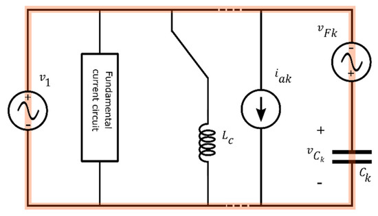
Figure 13.
KVL for obtaining the voltage across a capacitor adopted in the kth harmonic circuit.
According to this Kirchhoff’s voltage law (KVL), the voltage across the capacitors is imposed and then it is already at steady-state when the PSpice transient analysis starts.
The use of these capacitors asks for inserting a compensation inductor, LC, resonant at the fundamental frequency with the equivalent capacitor CEQ. As said before a resistor has to be added in series with the inductor to avoid the loop (LC − v1) which impedes simulation starts. Unfortunately, the current across this inductor is not yet at steady-state when the PSpice transient analysis starts, and recalling the standard expression of the current in a resistor-inductor circuit:
it is evident that the smaller the resistance the greater the time required to reach a steady state condition. In other words, the use of small resistance provides more accurate results but at the cost of long simulation time. To solve this problem, the initial condition value has to nullify the transient current across the compensation inductor, LC, that is:
Given the expression of the current across the inductor at steady-state when R→0, that implies :
the initial condition to be set is easily obtained:
To nullify the effect of Rloop (which is not present in the proposed model), a voltage controlled voltage source (VCVS) is placed in series with the resistor. More specifically, it is controlled by the voltage across the resistor with a gain equal to –1, thus obtaining that the following relation is valid for any resistance value Figure 14:
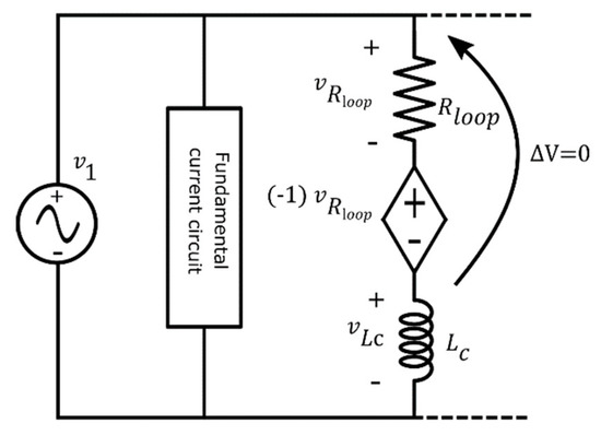
Figure 14.
VCCS that nullifies the effect of Rloop, thus obtaining a PSpice circuit that actually implements the proposed model.
Therefore, setting the initial condition equal to zero enables a steady-state current through the inductor when the PSpice transient analysis starts, regardless the value of Rloop. Moreover, nullifying the effect of the resistor enables to obtain a PSpice circuit that actually implements the proposed model. It is worth to noticing that the use of the VCVS without properly setting the initial condition enables to start the simulation but it does not address the underlining issues that lead PSpice to impede the simulation of circuit where a loop with only voltage sources and inductors is present. Finally, it is worth to recall that the steady-state current across the inductor has the same amplitude of the fundamental current flowing through the equivalent capacitor but these currents are in antiphase between them. Then the resulting fundamental current is zero which means, in turn, that the fundamental current flows only in the “fundamental current circuit”.
As said before, whether bq1 is positive, a capacitor is used in the “fundamental current circuit”, and then the voltage across it is equal to v1 according to the related KVL, then the voltage is also already at steady-state when the PSpice transient analysis starts. On the other hand, when bq1 is negative an inductor has to be adopted and, consequently, a resistor Rloop with the related VCVS has to be adopted and the initial condition has to be properly set (once again it has to be set equal to zero).
The mechanism adopted for these inductors can be readapted when Lk is used instead of Ck. At steady-state the voltage across the inductor is (Figure 15):

Figure 15.
A VCCS and a CCCS used to emulate, respectively, a short circuit and an open circuit when Lk is selected (that is d = 1, then Lk is connected in the lamp model while Ck is disconnected).
Then the steady-state current is:
Consequently, the initial condition to set in order to obtain a zero transient time for the current through the inductor is:
The switches in the model (Figure 9) have been emulated in PSpice with “voltage-controlled switch” (VCS) components. On the other hand, the VCS is not an ideal switch as the ones considered in the model. More specifically, a VCS is a resistor with a high resistance, ROFF, when it emulates the open-status while the closed-status is obtained by considering a low resistance, RON. The VCS resistance is set according the voltage value of the controlling nodes. It is worth noting that, the switch SR1 and SG1 (Figure 9) have to be controlled by the same voltage but with opposite logic since when the former is open the latter is closed, and vice versa. Therefore, to drive these switches, a fictitious constant voltage generator has been considered:
and:
A similar mechanism can be adopted for the couple of switches SL1-SC1, SCc-SLc, and SLk-SCk.
Regardless the status of a switch, the related resistance does not belong to the proposed model. Hence, similarly to Rloop, their effect should be nullified. It is worth noting, that the switch should ideally be a short-circuit when it is closed (that is, RON should be ideally zero). Therefore, the insertion of a VCVS that nullifies the effect of RON indeed enables to emulate a short circuit (as shown in Figure 15), thus, once again, the PSpice circuit actually implements the proposed model. On the other hand, ROFF emulates an open-circuit and, consequently, the addition of the VCVS is undesired in such a case. Notwithstanding, as the VCVS nullifies the effect of RON, dually, a current controlled current source (CCCS) placed in parallel with ROFF enables nullifying its effect, that is, it enables obtaining the desired open circuit. More specifically, it is controlled by the current through the resistor with a gain equal to –1, thus obtaining that the circuit elements downstream from the switch have no effect on the current drawn from the lamp circuit model.
The parametric PSpice circuits of the generic model of an ESL are reported in Figure 16, Figure 17, Figure 18, Figure 19 and Figure 20. It is worth to noticing that all voltage and current waveforms have been previously defined in terms of the “cosine” function while PSpice adopts the “sine” function; hence π/2 has been added in all the independent generators used in the PSpice netlist. The phase shift of the harmonics has been accordingly modified accounting for the related frequency.

Figure 16.
Netlist of the overall lamp circuit.
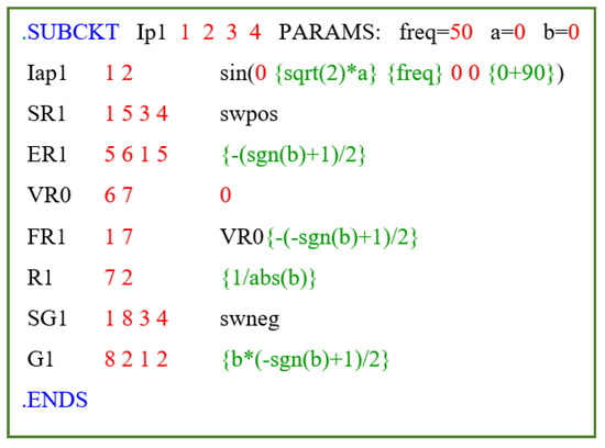
Figure 17.
Netlist of the active current circuit.
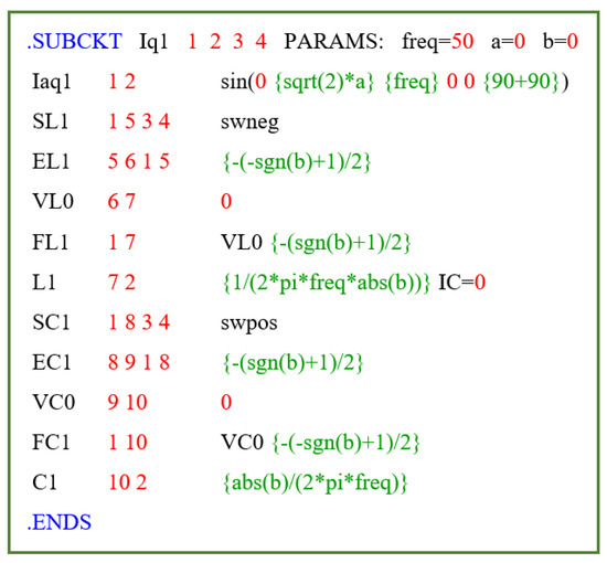
Figure 18.
Netlist of the reactive current circuit.
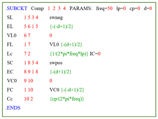
Figure 19.
Netlist of the compensation circuit.
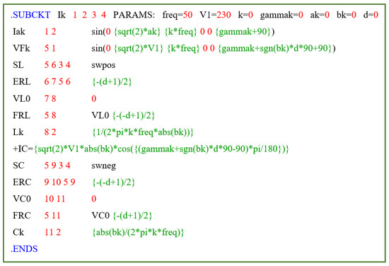
Figure 20.
Netlist of the generic harmonic circuit.
Figure 16 is the main PSpice circuit of a generic ESL, where “freq” is the fundamental frequency, V1 is the rms of the voltage on the main assumed to be purely sinusoidal and d is the aforesaid parameter used for considering an inductor (d = 1) or a capacitor (d = −1) in each harmonic subcircuit. The switches models “swpos” and “swneg” are used to emulate the complementary operated switches. They are used in combination with the fictitious independent generators Vbp1, Vbq1, and Vd to drive the couple of switches SR1-SG1, SL1-SC1, and SL-SC. Finally, Xp1, Xq1, and Xksim are the instances of, respectively, the active, reactive and harmonics currents, while X1 is the instance of the compensation subcircuit. The parameters ap1, bp1, aq1, bq1, ls, cs, gamma2, a2, b2, and so on, until gamma50, a50, and b50 can be reported in an external file for each lamp and then used with a “.INC” statement. The parameters ls and cs refer to the series in Equation (33).
Figure 17 reports the netlist related to the active current, where the nodes 1 and 2 are the local numbering of the lamp terminals (which are node 1 and 0 of the PSpice lamp model as evident from the instance Xp1 in Figure 16); the nodes 3 and 4 are the local numbering of the terminals (which are node 2 and 0 of the PSpice lamp model) of the voltage controlling the switches status; “freq” is the fundamental frequency (50 Hz is the default value); a and b are aP1 and bP1. Then, the actual nodes numbering as well as the parameter values depend on the calling instance Xp1. SR1 and SG1 are the switches complementary operated to ensure that only one between the resistor, R1, and the VCCS are connected. The following explanation refers to the local numbering.
When bp1 is a positive number the voltage across terminals 3–4 is 1 V, consequently SR1 and SG1 are equivalent to resistors with resistance equal to, respectively, 1 μΩ (that is ron) and 1 GΩ (that is roff). Moreover, the expression in the curly brackets of the VCVS ER1 is equal to −1, while it is 0 for the CCCS FR1 (it is an open circuit). Consequently, the voltage between nodes 1–6 is equal to 0, which implies a voltage across the resistor equal to the voltage on the mains (nodes 1–2) being also 0, the voltage between nodes 6–7. At the same time, the expression in the curly brackets of the VCCS G1 is equal to 0.
The behaviour of SR1 and SG1 is dual to the previous one when bq1 is a negative number because, in such a case, the voltage across the terminals 3–4 is −1 V. Moreover, the expression in the curly brackets of the CCCS FR1 is equal to −1, while is 0 for the VCVS ER1. Consequently, no current flows through R1 according the Kirchhoff’s Current Law (KCL) at node 7. At the same time, the expression in the curly brackets of the VCCS G1 is equal to the value of bp1. Therefore, only G1 is actually connected in the lamp circuit.
Similar considerations are valid for the other subcircuits. When a switch is closed, the VCVS in series with it presents a gain −1 that ensures the switch is equivalent to a short circuit (in this case the CCCS has gain equal to 0, then it has not any effect). The complementary switch is open, hence, its VCVS presents a gain equal to 0, having no effect, while the CCCS has a gain equal to −1 to ensure the switch behaves like to an open circuit.
4. Results
The comparison between the measured and simulated current waveforms of different ESLs have been carried out. The results have highlighted the high fidelity level of the proposed PSpice model in emulating the current drawn by the lamps under variable voltage on the mains. In the following the comparison between simulations and measurements have been reported for one CFL and one LED light bulb.
Figure 21, Figure 22, Figure 23 and Figure 24 report the measured voltage on the mains (blue waveform), the measured current (green waveform) and the simulated current (red waveform) for the two lamps when the rms voltage on the mains is, respectively, 212 V and 237 V. These two voltage levels have not been used for obtaining the parameters of the interpolation function, since these measurements have been performed only for model validation. They have been set by means of the variac similarly to the voltage level used for the interpolation functions as described before.
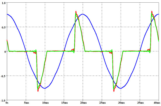
Figure 21.
Measured voltage on the mains (blue waveform, rms 212 V), measured current (green waveform) and simulated current (red waveform) for a CFL. Per-unit system: base voltage 400 V, base current 250 mA.
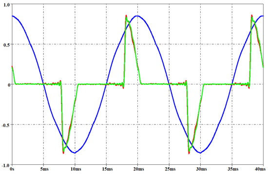
Figure 22.
Measured voltage on the mains (blue waveform, rms 237 V), measured current (green waveform) and simulated current (red waveform) for a CFL. Per-unit system: base voltage 400V, base current 250 mA.
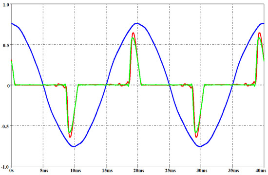
Figure 23.
Measured voltage on the mains (blue waveform, rms 212 V), measured current (green waveform) and simulated current (red waveform) for a LED. Per-unit system: base voltage 400 V, base current 300 mA.
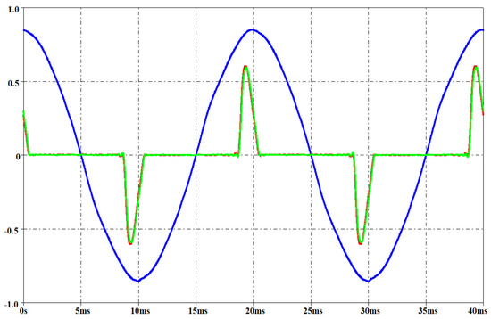
Figure 24.
Measured voltage on the mains (blue waveform, rms 237 V), measured current (green waveform) and simulated current (red waveform) for a LED. Per-unit system: base voltage 400 V, base current 300 mA.
The simulated currents that are reported in the figures have been obtained using the inductors in the harmonic subcircuits (i.e., d = 1). The results confirm that the current is already at steady-state when the transient analysis starts, then the method adopted for the PSpice implementation of the current lamp model is effective. By analyzing the figures, the goodness of the proposed PSpice model is also evident. Moreover, the results shown a slightly better current estimation for the CFL with respect to the LED light bulb when the voltage on the mains is less than the rated one. On the other hand, the predicted current is more accurate for the LED light bulb in case of voltage on the mains exceeding the nominal value. As expected, there was not any difference between the voltage THD during the current measurement (lamp on) and without any load (lamp off). The THD of the voltage on the mains was in the interval 2–4% during the measurements.
The total number of circuit components in the active and reactive current circuit is, respectively, 8 and 11 (Figure 17 and Figure 18). The compensation circuit includes 10 components (Figure 19), while there are 12 components in each harmonic subcircuit (Figure 20). Therefore, the total number of components of the lamp PSpice circuit is 617 when the current harmonics, until the 50th, are used. On the other hand, a reduced circuit can be obtained using a less general circuit where each switch with the related zero-voltage generator, VCVS, and CCCS are removed together with the elements to be disconnected. In such a case the number of components in the active current circuit is 2. The number of component in the reactive current circuit is also 2 when the capacitor has to be considered (bq1 is positive), while it is 4 when the inductor has to be considered since a resistor, Rloop, and the related VCVS have to be considered. The adoption of only capacitors or only inductors in the harmonic subcircuit reduces its number of component to three in the first case, while five components in the second one are due to the need of the resistor and VCVS. Finally, only the capacitor is adopted in the compensation circuit when the inductors are used in the harmonic subcircuits, while three components are necessary when an inductor has to compensate the equivalent capacitance of the harmonic subcircuits. Therefore, the smallest reduced lamp circuit has 154 components, while 252 components are present in the greatest reduced circuit. It is worth noting that the reduced circuits provide the same current waveform of the one with 617 (full circuit) but each reduced circuit is related only to a given lamp.
Neglecting a current harmonic enables to remove 12 components from the full circuit (three or five in the reduced ones) at the cost of worsening the model accuracy. The error on the current THD described before has been used as criterion for choosing the harmonic to be considered. Two levels of maximum THD error have been considered: 1% and 10%. It is worth noticing that each time a group of harmonics is neglected and the related components removed from the PSpice circuit the value of LEQ (or CEQ) changes, then the resonant (at the fundamental frequency) component in the compensation circuit has to be properly accorded. Figure 25, Figure 26, Figure 27 and Figure 28 report the measured current (green waveform) and the simulated current involving a THD error of 1% (red waveform) and 10% (blue waveform) for both lamps at the two aforementioned voltage levels adopted for model validation. The harmonics neglected for achieving a given THD error refer to Figure 5, Figure 6, Figure 7 and Figure 8. It is worth noting that the reduced circuit performing a THD error of 1% contains less than 40 components. The electrical components used in the PSpice circuit to obtain the current waveforms involving a THD error of 10% are summarized in Appendix A.
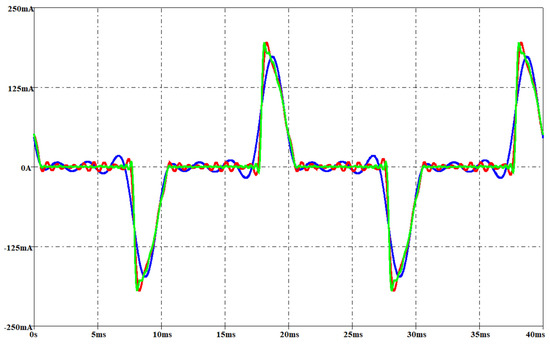
Figure 25.
CFL: measured current (green waveform) and the simulated current involving a THD error of 1% (red waveform) and 10% (blue waveform) with an rms voltage of 212 V.
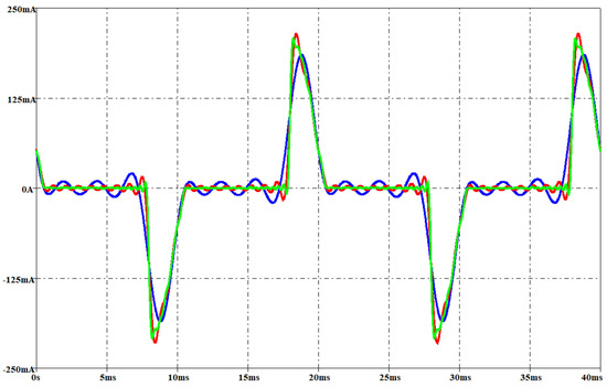
Figure 26.
CFL: measured current (green waveform) and the simulated current involving a THD error of 1% (red waveform) and 10% (blue waveform) with an rms voltage of 237 V.
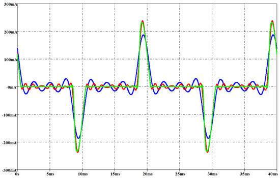
Figure 27.
LED lamp: measured current (green waveform) and the simulated current involving a THD error of 1% (red waveform) and 10% (blue waveform) with an rms voltage of 212 V.
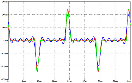
Figure 28.
LED lamp: measured current (green waveform) and the simulated current involving a THD error of 1% (red waveform) and 10% (blue waveform) with an rms voltage of 237 V.
At 212 V, the simulated currents involve about the same accuracy level for both lamps in case of 1% THD error. On the other hand, the comparison of the predicted currents in case of 10% THD error points out that the CFL current is more accurately esteemed. For both lamps and THD errors, the “flat zone” in the measured current waveform is poorly approximated although the CFL current is more accurate. The “hills” in the measured current waveform are well approximated for both lamps in case of 1% THD error, while a poor result is obtained in case of 10% THD error. At 237 V, the simulated currents are more accurate that the other voltage level in case of 1% THD error. In such a case, the simulated waveform of the LED current is more accurate than the. On the other hand, in case of 10% THD error, the “flat zone” in the simulated waveform of the CFL current is better than the LED one, while the LED outperforms the CFL in the “hill” estimation.
5. Conclusions
The reduction of the distorted current injected on the mains by energy-saving lamps is necessary, especially in case of large lighting systems or smart lighting systems implementing several functionalities. Optimal lighting system design aiming at harmonics cancellation is the most economical solution, but it needs a tool able to predict the current drawn from each lamp also considering the variation of the voltage on the mains. A parametric PSpice circuit has been proposed to predict the current waveform of any lamp on the market once few measurements are performed. The underlying theory, equations, rules, and procedures, as well as the parametric netlist, have been reported. The key features enabling to overcome the limitations of other circuit models is that the proposed parametric PSpice circuit does not need any information about the lamp driver and components since each lamp is treated as a black box when the lamp parameters have to be computed. A further advantage of the method over previous works is the use of a linear circuit that enables low computational cost and fast simulation. The results have confirmed the high accuracy level of the PSpice circuit in predicting the current waveform even when a reduced circuit is adopted and various harmonics are neglected.
Author Contributions
All authors contributed equally to this work.
Funding
This research received no external funding.
Conflicts of Interest
The authors declare no conflict of interest.
Nomenclature
| [V] | Fundamental frequency of the voltage on the main. | |
| [A] | Fundamental frequency of the current drawn by the lamp. | |
| [A] | kth current harmonic | |
| [A] | Active current | |
| [A] | Reactive current | |
| [A] | Current that takes into account the term | |
| [A] | Current that takes into account the term | |
| [A] | Current that takes into account the term | |
| [A] | Current that takes into account the term | |
| [A] | Current that takes into account the term | |
| [A] | Current that takes into account the term | |
| [V] | Fictitious voltage independent generator | |
| [Ω] | Compensation component | |
| [Ω] | On/Off resistance of a Voltage Controlled Switch |
| Intercept of the interpolation function of the active current (rms) | |
| Slope of the interpolation function of the active current (rms) | |
| Intercept of the interpolation function of the reactive current (rms) | |
| Slope of the interpolation function of the reactive current (rms) | |
| Intercept of the interpolation function of the current (rms) harmonics | |
| Slope of the interpolation function of the current (rms) harmonics |
Appendix A
The electrical components used in PSpice circuit to obtain some current waveforms reported in the “Results” section are summarized in this appendix. In Table A1 are reported the values of the electrical components of the PSpice circuit of the CFL when it has been considered the 10% THD error, and in Table A2 the LED lamp quantities in the case.

Table A1.
Quantities used in the PSpice circuit of a CFL under test in case of 10% THD error.
Table A1.
Quantities used in the PSpice circuit of a CFL under test in case of 10% THD error.
| Quantity | Value | Quantity | Value | Quantity | Value |
|---|---|---|---|---|---|
| IaP1 | 41.64 mA | Lc | 56.90 H | φ5 | 107° |
| IaQ1 | 27.61 mA | Cc | 24.52 µF | L5 | 9.98 H |
| φ1 | 90° | SCc | closed | C5 | 40.63 µF |
| R1 | 355.81 kΩ | SLc | open | SL5 | closed |
| G1 | 2.81 µΩ−1 | Ia3 | 34.71 mA | SC5 | open |
| SR1 | closed | φ3 | 62° | Ia7 | 5.82 mA |
| SG1 | open | L3 | 62.08 H | Φ7 | 162° |
| L1 | 64.31 H | C3 | 18.15 µF | L7 | 4.62 H |
| C1 | 0.16 µF | SL3 | closed | C7 | 44.72 µF |
| SL1 | closed | SC3 | open | SL7 | closed |
| SC1 | open | Ia5 | 13.34 mA | SC7 | open |
Table A2.
Quantities used in the PSpice circuit of a LED under test in case of 10% THD error.
Table A2.
Quantities used in the PSpice circuit of a LED under test in case of 10% THD error.
| Quantity | Value | Quantity | Value | Quantity | Value |
|---|---|---|---|---|---|
| IaP1 | 72.07 mA | Lc | 34.35 H | φ5 | 47° |
| IaQ1 | 21.65 mA | Cc | 26.32 µF | L5 | 6.07H |
| φ1 | 90° | SCc | closed | C5 | 68.81 µF |
| R1 | 6.33 kΩ | SLc | open | SL5 | closed |
| G1 | 157.9 µΩ−1 | Ia3 | 67.43 mA | SC5 | open |
| SR1 | open | φ3 | 35° | Ia7 | 37.98 mA |
| SG1 | closed | L3 | 7.32 H | Φ7 | 68° |
| L1 | 46.42 H | C3 | 1.53 µF | L7 | 8.18 H |
| C1 | 0.21 µF | SL3 | closed | C7 | 15.80 µF |
| SL1 | closed | SC3 | open | SL7 | closed |
| SC1 | open | Ia5 | 54.42 mA | SC7 | open |
References
- Hoseini, A.; Dahlan, N.; Berardi, U.; Hoseini, A.; Makaremi, N.; Hoseini, M. Sustainable energy performances of green buildings: A review of current theories, implementations and challenges. Renew. Sustain. Energy Rev. 2013, 25, 1–17. [Google Scholar] [CrossRef]
- Yu, Y.; Wang, X.; Li, H.; Qi, Y.; Tamura, K. Ex-post assessment of China’s industrial energy efficiency policies during the 11th Five-Year Plan. Energy Policy 2015, 76, 132–145. [Google Scholar] [CrossRef]
- Ringel, M.; Schlomann, B.; Krail, M.; Rohde, C. Towards a green economy in Germany? The role of energy efficiency policies. Appl. Energy 2016, 179, 1293–1303. [Google Scholar] [CrossRef]
- Bye, B.; Fæhn, T.; Rosnes, O. Residential energy efficiency policies: Costs, emissions and rebound effects. Energy 2018, 143, 191–201. [Google Scholar] [CrossRef]
- Santos, A.; Fagá, M.; Santos, E. The risks of an energy efficiency policy for buildings based solely on the consumption evaluation of final energy. Int. J. Electr. Power Energy Syst. 2013, 44, 70–77. [Google Scholar] [CrossRef]
- Brown, M. Innovative energy-efficiency policies: An international review. Wiley Interdiscip. Rev. Energy Environ. 2015, 4, 1–25. [Google Scholar] [CrossRef]
- Perea-Moreno, M.; Manzano-Agugliaro, F.; Perea-Moreno, A.-J. Sustainable Energy Based on Sunflower Seed Husk Boiler for Residential Buildings. Sustainability 2018, 10, 3407. [Google Scholar] [CrossRef]
- Bladh, M. Energy efficient lighting meets real home life. Energy Effic. 2011, 4, 35–245. [Google Scholar] [CrossRef]
- Dixon, R.K.; McGowan, E.; Onysko, G.; Scheer, R.M. US energy conservation and efficiency policies: Challenges and opportunities. Energy Policy 2010, 38, 6398–6408. [Google Scholar] [CrossRef]
- Karlicek, R.F. Smart lighting—More than illumination. In Proceedings of the Asia Communications and Photonics Conference (ACP), Guangzhou, China, 7–10 November 2012. [Google Scholar]
- Patil, K.D.; Gandhare, W.Z. Effects of harmonics in distribution systems on temperature rise and life of XLPE power cables. In Proceedings of the International Conference on Power and Energy Systems, Chennai, India, 22–24 December 2011; pp. 1–6. [Google Scholar]
- Wu, J.-C.; Jou, H.-L.; Wu, K.-D.; Shen, N.C. Power converter-based method for protecting three-phase power capacitor from harmonic destruction. IEEE Trans. Power Deliv. 2004, 19, 1434–1441. [Google Scholar] [CrossRef]
- Lin, S.; Salles, D.; Freitas, W.; Xu, W. An Intelligent Control Strategy for Power Factor Compensation on Distorted Low Voltage Power Systems. IEEE Trans. Smart Grid 2012, 3, 1562–1570. [Google Scholar] [CrossRef]
- Cheng, C.-A.; Chang, E.C.; Tseng, C.-H.; Chung, T.-Y. A Single-Stage LED Tube Lamp Driver with Power-Factor Corrections and Soft Switching for Energy-Saving Indoor Lighting Applications. Appl. Sci. 2017, 7, 115. [Google Scholar] [CrossRef]
- Chang, Y.-N.; Chan, S.-Y.; Cheng, H.-L. A Single-Stage High-Power Factor Converter with Synchronized Self-Excited Technique for LED Lighting. Appl. Sci. 2018, 8, 1408. [Google Scholar] [CrossRef]
- Said, D.M.; Nor, K.M.; Majid, M.S. Analysis of distribution transformer losses and life expectancy using measured harmonic data. In Proceedings of the 14th International Conference on Harmonics and Quality of Power—ICHQP 2010, Bergamo, Italy, 26–29 September 2010; pp. 1–6. [Google Scholar]
- Dao, T.; Phung, B.T.; Blackburn, T. Effects of voltage harmonics on distribution transformer losses. In Proceedings of the IEEE PES Asia-Pacific Power and Energy Engineering Conference (APPEEC), Brisbane, Australia, 15–18 November 2015; pp. 1–5. [Google Scholar]
- Serov, A.N.; Shatokhin, A.A.; Gerasimov, S.I. The Impact of Power Harmonics and Noise on the Measurement Error of the Frequency by Derivative Technique. In Proceedings of the Renewable Energies, Power Systems & Green Inclusive Economy (REPS-GIE), Casablanca, Morocco, 23–24 April 2018; pp. 1–5. [Google Scholar]
- Watson, N.R.; Scott, T.; Hirsch, S. Compact fluorescent lamps (CFL)—Implications for distribution networks. In Proceedings of the EEA Conference, Auckland, New Zealand, June 2006. [Google Scholar]
- Chuang, Y.; Ke, Y.; Chuang, H.; Hu, C. Single-Stage Power-Factor-Correction Circuit with Flyback Converter to Drive LEDs for Lighting Applications. In Proceedings of the IEEE Industry Applications Society Annual Meeting, Houston, TX, USA, 3–7 October 2010; pp. 1–9. [Google Scholar]
- Karim, F.A.; Ramdhani, M.; Kurniawan, E. Low pass filter installation for reducing harmonic current emissions from LED lamps based on EMC standard. In Proceedings of the International Conference on Control, Electronics, Renewable Energy and Communications (ICCEREC), Bandung, Indonesia, 13–15 September 2016; pp. 132–135. [Google Scholar]
- Sarwono, E.; Facta, M.; Handoko, S. Investigation of Passive Filter for LED Lamp. IOP Conf. Ser. Mater. Sci. Eng. 2017. [Google Scholar] [CrossRef]
- Ann, M.M.; Sudhakar, T.D.; Mohanadasse, K.; Sharmeela, C. Performance comparison of electronic ballast topologies for low power compact fluorescent lamp application. In Proceedings of the International Conference on Circuits, Power and Computing Technologies [ICCPCT], Nagercoil, India, 20–21 March 2014; pp. 1251–1256. [Google Scholar]
- Prabha, S.U.; Srinivasan, M.; Keerthana, C. Reduction of total harmonic distortion in electronic ballast. In Proceedings of the International Conference on Innovations in Electrical, Electronics, Instrumentation and Media Technology (ICEEIMT), Coimbatore, India, 3–4 February 2017; pp. 62–65. [Google Scholar]
- Hassanzadeh, M.; Sheikholeslami, A.; Ghoreishi, H.; Mohseni, S.; Nazari, M. A novel method for current harmonic reduction of CFLs in large number usage. In Proceedings of the 6th Power Electronics, Drive Systems & Technologies Conference (PEDSTC2015), Tehran, Iran, 3–4 February 2015; pp. 424–429. [Google Scholar]
- Nassif, A.B.; Xu, W. Characterizing the Harmonic Attenuation Effect of Compact Fluorescent Lamps. IEEE Trans. Power Deliv. 2009, 24, 1748–1749. [Google Scholar] [CrossRef]
- Ćuk, V.; Cobben, J.F.G.; Kling, W.L.; Timens, R.B. An analysis of diversity factors applied to harmonic emission limits for energy saving lamps. In Proceedings of the 14th International Conference on Harmonics and Quality of Power, Bergamo, Italy, 26–29 September 2010; pp. 1–6. [Google Scholar]
- Uddin, S.; Shareef, H.; Mohamed, A.; Hannan, M.A. An analysis of harmonic diversity factors applied to LED lamps. In Proceedings of the IEEE International Conference on Power System Technology (POWERCON), Auckland, New Zeland, 30 October–2 November 2012; pp. 1–5. [Google Scholar]
- Gil-de-Castro, A.; Rönnberg, S.; Bollen, M.H.J.; Moreno-Muñoz, A.; Pallares-Lopez, V. Harmonics from a domestic customer with different lamp technologies. In Proceedings of the IEEE 15th International Conference on Harmonics and Quality of Power, Hong Kong, China, 17–20 June 2012; pp. 585–590. [Google Scholar]
- Yeh, E.; Venkata, S.S.; Sumic, Z. Improved distribution system planning using computational evolution. IEEE Trans. Power Syst. 1996, 11, 668–674. [Google Scholar] [CrossRef]
- Soori, P.K.; Vishwas, M. Lighting control strategy for energy efficient office lighting system design. Energy Build. 2013, 66, 329–337. [Google Scholar] [CrossRef]
- Mukherjee, P. An Overview of Energy Efficient Lighting System Design for Indoor Applications of an Office Building. Key Eng. Mater. 2016, 692, 45–53. [Google Scholar] [CrossRef]
- Alzubaidi, S.; Soori, P.K. Energy Efficient Lighting System Design for Hospitals Diagnostic and Treatment Room—A Case Study. J. Light Vis. Environ. 2012, 36, 23–31. [Google Scholar] [CrossRef]
- Byun, J.; Shin, T. Design and Implementation of an Energy-Saving Lighting Control System Considering User Satisfaction. IEEE Trans. Consum. Electron. 2018, 64, 61–68. [Google Scholar] [CrossRef]
- Soori, P.K.; Alzubaidi, S. Study on improving the energy efficiency of office building’s lighting system design. In Proceedings of the IEEE GCC Conference and Exhibition (GCC), Dubai, USA, 19–22 February 2011; pp. 585–588. [Google Scholar]
- Wagiman, K.R.; Abdullah, M.N. Lighting system design according to different standards in office building: A technical and economic evaluations. J. Phys. Conf. Ser. 2018, 1049. [Google Scholar] [CrossRef]
- Wang, L.; Li, H.; Zou, X.; Shen, X. Lighting system design based on a sensor network for energy savings in large industrial buildings. Energy Build. 2015, 105, 226–235. [Google Scholar] [CrossRef]
- Muhamad, W.N.W.; Zain, M.Y.M.; Wahab, N.; Aziz, N.H.A.; Kadir, R.A. Energy Efficient Lighting System Design for Building. In Proceedings of the International Conference on Intelligent Systems, Modelling and Simulation, Liverpool, UK, 27–29 January 2010; pp. 282–286. [Google Scholar]
- Liang, L.; Tian, H.; Ning, P. Artificial light LED planting system design. In Proceedings of the 14th China International Forum on Solid State Lighting: International Forum on Wide Bandgap Semiconductors China (SSLChina: IFWS), Beijing, China, 1–3 November 2017; pp. 88–90. [Google Scholar]
- Kuo, W.; Chiang, C.; Huang, Y. An Automatic Light Monitoring System with Light-to-Frequency Converter for Flower Planting. In Proceedings of the IEEE Instrumentation and Measurement Technology Conference, Victoria, BC, Canada, 12–15 May 2008; pp. 1146–1149. [Google Scholar]
- Olvera-Gonzalez, E.; Alaniz-Lumbreras, D.; Torres, V.; González-Ramírez, E.; De Jesús Hernández, J.; Araiza, M.; Tsonchev, R.; Olvera-Olvera, C.; Castaño, V. A LED-based smart illumination system for studying plant growth. Light. Res. Technol. 2014, 46, 128–139. [Google Scholar] [CrossRef]
- Khamis, M.N.; Ismail, N.F.; Yunus, N.A.M.; Ahmad, D. LED lighting with remote monitoring and controlling system for indoor greenhouse. In Proceedings of the IEEE Asia Pacific Conference on Postgraduate Research in Microelectronics and Electronics (PrimeAsia), Kuala Lumpur, Malaysia, 31 October–2 November 2017; pp. 81–84. [Google Scholar]
- Dilettoso, E.; Rizzo, S.A.; Salerno, N. A Parallel Version of the Self-Adaptive Low-High Evaluation Evolutionary-Algorithm for Electromagnetic Device Optimization. IEEE Trans. Magn. 2014, 50, 633–636. [Google Scholar] [CrossRef]
- Santiago, R.M.C.; Jose, J.A.; Bandala, A.A.; Dadios, E.P. Multiple objective optimization of LED lighting system design using genetic algorithm. In Proceedings of the International Conference on Information and Communication Technology, Malacca City, Malaysia, 17–19 May 2017; pp. 1–5. [Google Scholar]
- Ferentinos, K.P.; Albright, L.D. Optimal design of plant lighting system by genetic algorithms. Eng. Appl. Artif. Intell. 2005, 18, 473–484. [Google Scholar] [CrossRef]
- Cheng, C.-A.; Chang, C.-H.; Cheng, H.-L.; Tseng, C.-H.; Chung, T.-Y. A Single-Stage High-Power-Factor Light-Emitting Diode (LED) Driver with Coupled Inductors for Streetlight Applications. Appl. Sci. 2017, 7, 167. [Google Scholar] [CrossRef]
- Bender, V.C.; Mendes, F.B.; Maggi, T.; Dalla Costa, M.A.; Marchesan, T.B. Design methodology for street lighting luminaires based on a photometrical analysis. In Proceedings of the Brazilian Power Electronics Conference, Gramado, Brasil, 27–31 October 2013; pp. 1160–1165. [Google Scholar]
- Chu, C.-W.; Chao, W.-C.; Yang, C.-C.; Wu, P.-J.; Chen, C.-Y.; Kuo, Y.-P.; Lee, L.-L. Optimal Design of LED Street Lighting with Road Conditions. In Proceedings of the Third International Conference on Computing Measurement Control and Sensor Network (CMCSN), Matsue, Japan, 20–22 May 2016; pp. 9–11. [Google Scholar]
- Sun, C. Design of LED Street Lighting Adapted for Free-Form Roads. IEEE Photonics J. 2017, 9, 1–13. [Google Scholar] [CrossRef]
- Yao, Q.; Wang, H.; Uttley, J.; Zhuang, X. Illuminance Reconstruction of Road Lighting in Urban Areas for Efficient and Healthy Lighting Performance Evaluation. Appl. Sci. 2018, 8, 1646. [Google Scholar] [CrossRef]
- Xu, X.; Collin, A.; Djokic, S.Z.; Langella, R.; Testa, A.; Drapela, J. Experimental evaluation and classification of LED lamps for typical residential applications. In Proceedings of the IEEE PES Innovative Smart Grid Technologies Conference Europe (ISGT-Europe), Torino, Italy, 26–29 September 2017; pp. 1–6. [Google Scholar]
- Saxena, R.; Nikum, K. Comparative study of different residential illumination appliances based on power quality. In Proceedings of the IEEE 5th India International Conference on Power Electronics (IICPE), Delhi, India, 6–8 December 2012; pp. 1–5. [Google Scholar]
- Swami, H.; Jain, A.K.; Azad, I.H.; Meena, N. Evaluation of input harmonic characteristics of LED lamps connected to utility grid. In Proceedings of the IEEMA Engineer Infinite Conference, New Delhi, India, 13–14 March 2018; pp. 1–6. [Google Scholar]
- Rönnberg, S.K.; Wahlberg, M.; Bollen, M.H.J. Harmonic emission before and after changing to LED and CFL—Part II: Field measurements for a hotel. In Proceedings of the 14th International Conference on Harmonics and Quality of Power, Bergamo, Italy, 26–29 September2010; pp. 1–6. [Google Scholar]
- Rönnberg, S.K.; Wahlberg, M.; Bollen, M.H.J. Harmonic emission before and after changing to LED lamps—Field measurements for an urban area. In Proceedings of the IEEE 15th International Conference on Harmonics and Quality of Power, Hong Kong, China, 17–20 June 2012; pp. 552–557. [Google Scholar]
- Rönnberg, S.K.; Wahlberg, M.; Bollen, M.H.J. Harmonic emission before and after changing to LED and CFL—Part I: Laboratory measurements for a domestic customer. In Proceedings of the 14th International Conference on Harmonics and Quality of Power, Bergamo, Italy, 26–29 September 2010; pp. 1–7. [Google Scholar]
- Shabbir, H.; Ur Rehman, M.; Rehman, S.A.; Sheikh, S.K.; Zaffar, N. Assessment of harmonic pollution by LED lamps in power systems. In Proceedings of the Clemson University Power Systems Conference, Clemson, SC, USA, 11–14 March 2014; pp. 1–7. [Google Scholar]
- Adoghe, A.U.; Eberechukwu, O.C.; Sanni, T.F. The effect of low power factor led lamp invasion on the utility grid: A case study of Nigerian market. In Proceedings of the IEEE PES PowerAfrica, Accra, Ghana, 27–30 June 2017; pp. 413–417. [Google Scholar]
- Blanco, A.M.; Parra, E. Effects of high penetration of CFLS and LEDS on the distribution networks. In Proceedings of the 14th International Conference on Harmonics and Quality of Power, Bergamo, Italy, 26–29 September 2010; pp. 1–5. [Google Scholar]
- Watson, N.R.; Scott, T.L.; Hirsch, S.J.J. Implications for Distribution Networks of High Penetration of Compact Fluorescent Lamps. IEEE Trans. Power Deliv. 2009, 24, 1521–1528. [Google Scholar] [CrossRef]
- Pileggi, D.J.; Gulachenski, E.M.; Root, C.E.; Gentile, T.J.; Emanuel, A.E. The effect of modern compact fluorescent lights on voltage distortion. IEEE Trans. Power Deliv. 1993, 8, 1451–1459. [Google Scholar] [CrossRef]
- Embriz-Santander, E.; Domijan, A.; Williams, C.W. A comprehensive harmonic study of electronic ballasts and their effect on a utility’s 12 kV, 10 MVA feeder. IEEE Trans. Power Deliv. 1995, 10, 1591–1599. [Google Scholar] [CrossRef]
- Wei, Z.; Watson, N.R.; Frater, L.P. Modelling of compact fluorescent lamps. In Proceedings of the 13th International Conference on Harmonics and Quality of Power, Australia, 28 September–1 October 2008; pp. 1–6. [Google Scholar]
- Cunill-Sola, J.; Salichs, M. Study and Characterization of Waveforms From Low-Watt (<25 W) Compact Fluorescent Lamps with Electronic Ballasts. IEEE Trans. Power Deliv. 2007, 22, 2305–2311. [Google Scholar] [CrossRef]
- Nassif, A.B.; Yong, J.; Xu, W. Measurement-based approach for constructing harmonic models of electronic home appliances. IET Gener. Transm. Distrib. 2010, 4, 363–375. [Google Scholar] [CrossRef]
- Braga, D.S.; Jota, P.R.S. Prediction of total harmonic distortion based on harmonic modeling of nonlinear loads using measured data for parameter estimation. In Proceedings of the 17th International Conference on Harmonics and Quality of Power (ICHQP), Belo Horizonte, Brazil, 16–19 October 2016; pp. 454–459. [Google Scholar]
- Yong, J.; Chen, L.; Nassif, A.B.; Xu, W. A Frequency-Domain Harmonic Model for Compact Fluorescent Lamps. IEEE Trans. Power Deliv. 2010, 25, 1182–1189. [Google Scholar] [CrossRef]
- Molina, J.; Sainz, L. Model of Electronic Ballast Compact Fluorescent Lamps. IEEE Trans. Power Deliv. 2014, 29, 1363–1371. [Google Scholar] [CrossRef]
- Molina, J.; Mesas, J.J.; Sainz, L. Parameter estimation procedure for the equivalent circuit model of compact fluorescent lamps. Electr. Power Syst. Res. 2014, 116, 128–135. [Google Scholar] [CrossRef]
- Souza, R.R.N.; Coutinho, D.F.; Tonkoski, R.; Silva, S.L.C.; Telló, M.; Canalli, V.M.; Dias, G.A.D.; Lima, J.C.M.; Sarmanho, U.A.S.; Maizonave, G.B.; et al. Nonlinear Loads Parameters Estimation and Modeling. In Proceedings of the IEEE International Symposium on Industrial Electronics, Vigo, Spain, 4–7 June 2007; pp. 937–942. [Google Scholar]
- Mesas, J.; Sainz, L.; Molina, J. Parameter Estimation Procedure for Models of Single-Phase Uncontrolled Rectifiers. IEEE Trans. Power Deliv. 2011, 26, 1911–1919. [Google Scholar] [CrossRef]
- Maza-Ortega, J.M.; Gómez-Expósito, A.; Trigo-García, J.L.; Burgos-Payán, M. Parameter estimation of harmonic polluting industrial loads. Int. J. Electr. Power Energy Syst. 2005, 27, 635–640. [Google Scholar] [CrossRef]
- Monjo, L.; Mesas, J.J.; Sainz, L.; Pedra, J. Study of voltage sag impact on LED lamp consumed currents. In Proceedings of the International Symposium on Fundamentals of Electrical Engineering (ISFEE), Bucharest, Romania, 30 June–2 July 2016; pp. 1–6. [Google Scholar]
- IEEE-1459-2010 Standard—IEEE Standard Definitions for the Measurements of Electric Power Quantities under Sinusoidal, Nonsinusoidal, Balanced or Unbalanced Conditions; IEEE: New York, NY, USA, 2010.
- Di Mauro, S.; Raciti, A.; Rizzo, S.A.; Susinni, G. LED lamp PSpice circuit emulating first harmonic current absorption as a function of the main voltage. In Proceedings of the 2018 International Symposium on Power Electronics, Electrical Drives, Automation and Motion (SPEEDAM), Amalfi, Italy, 20–22 June 2018; pp. 1101–1106. [Google Scholar]
- Raciti, A.; Rizzo, S.A.; Susinni, G. Steady-State Electrical Modeling of LED and CF Bulb Lamps under Variable Voltage on the Main. In Proceedings of the 2018 IEEE International Conference on Environment and Electrical Engineering and IEEE Industrial and Commercial Power Systems Europe (EEEIC/I&CPS Europe), Palermo, Italy, 12–15 June 2018; pp. 1–6. [Google Scholar]
- Alobeidli, K.; Syed, M.; El Moursi, M.; Zeineldin, H. Novel Coordinated Voltage Control for Hybrid Micro-Grid with islanding capability. IEEE Trans. Smart Grid 2015, 6, 1116–1127. [Google Scholar] [CrossRef]
- Pasha, A.M.; Zeineldin, H.; Saad, A.; Sumaiti, A.; El Moursi, M.S.; El Sadaany, E.F. Conservation Voltage Reduction for Autonomous Microgrids Based on V–I Droop Characteristics. IEEE Trans. Sustain. Energy 2017, 8, 1076–1085. [Google Scholar] [CrossRef]
- Tech, H.; Leber, D.; Schwarzmeier, A. A novel approach to efficient inrush current limitation for LED power applications. In Proceedings of the PCIM Europe 2014: International Exhibition and Conference for Power Electronics, Intelligent Motion, Renewable Energy and Energy Management, Nuremberg, Germany, 20–22 May 2014; pp. 1–8. [Google Scholar]
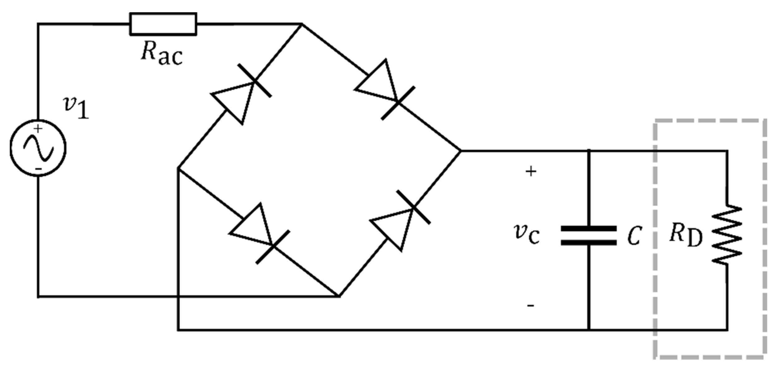
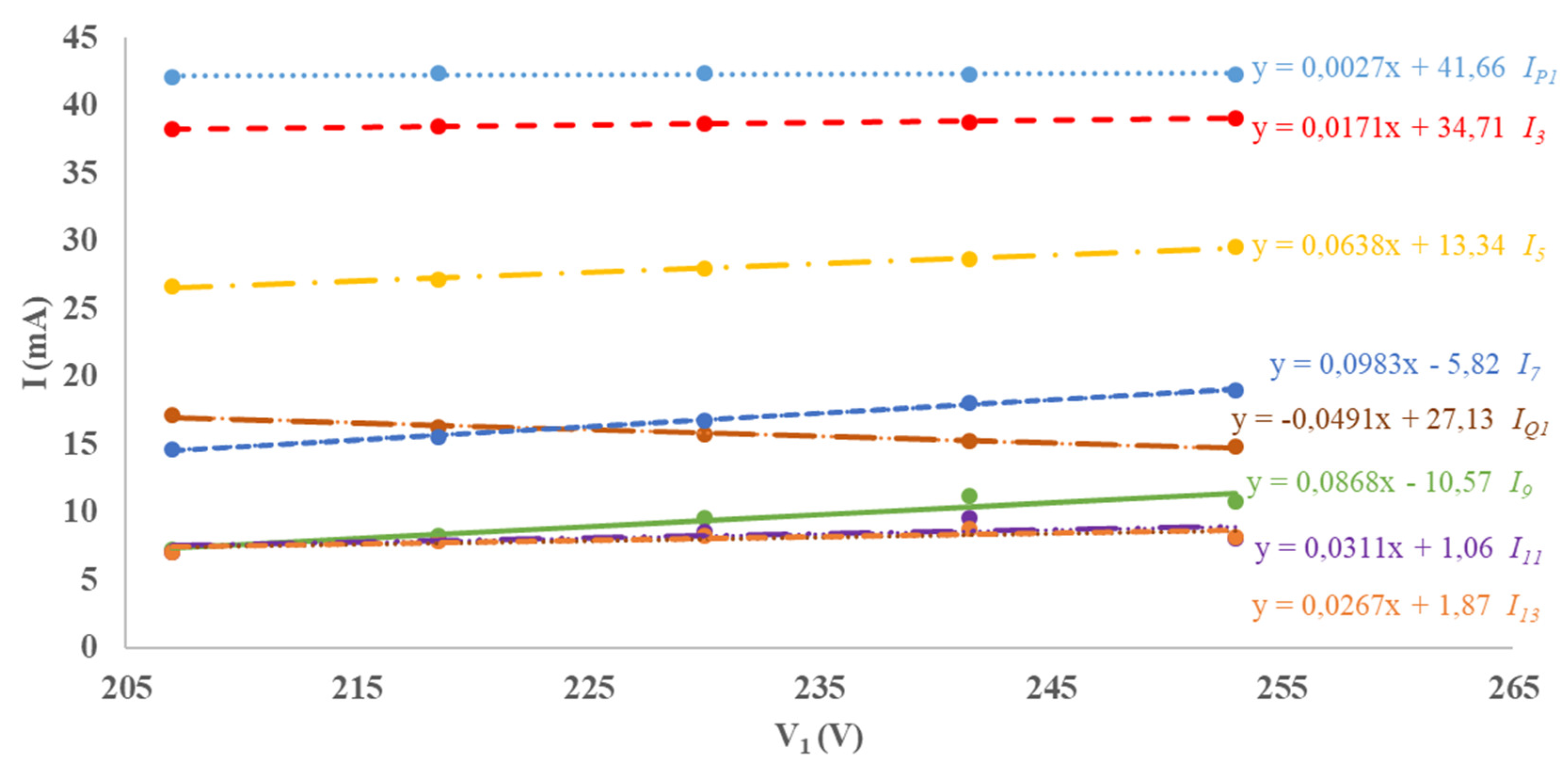
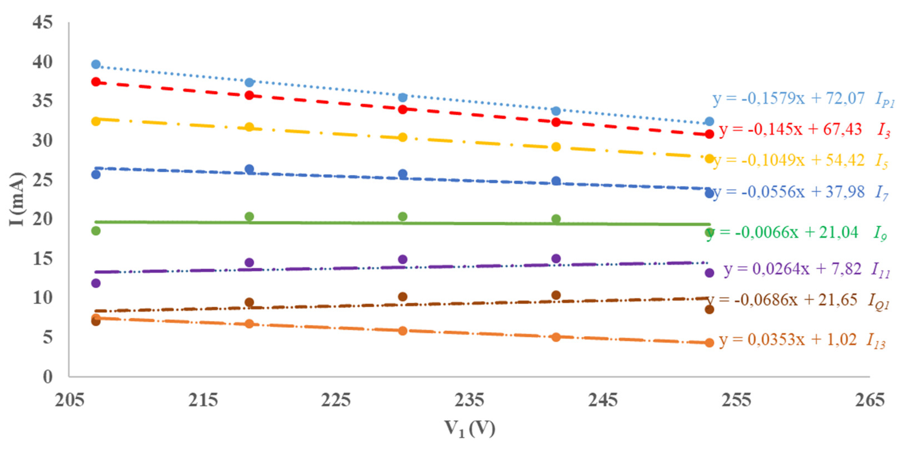
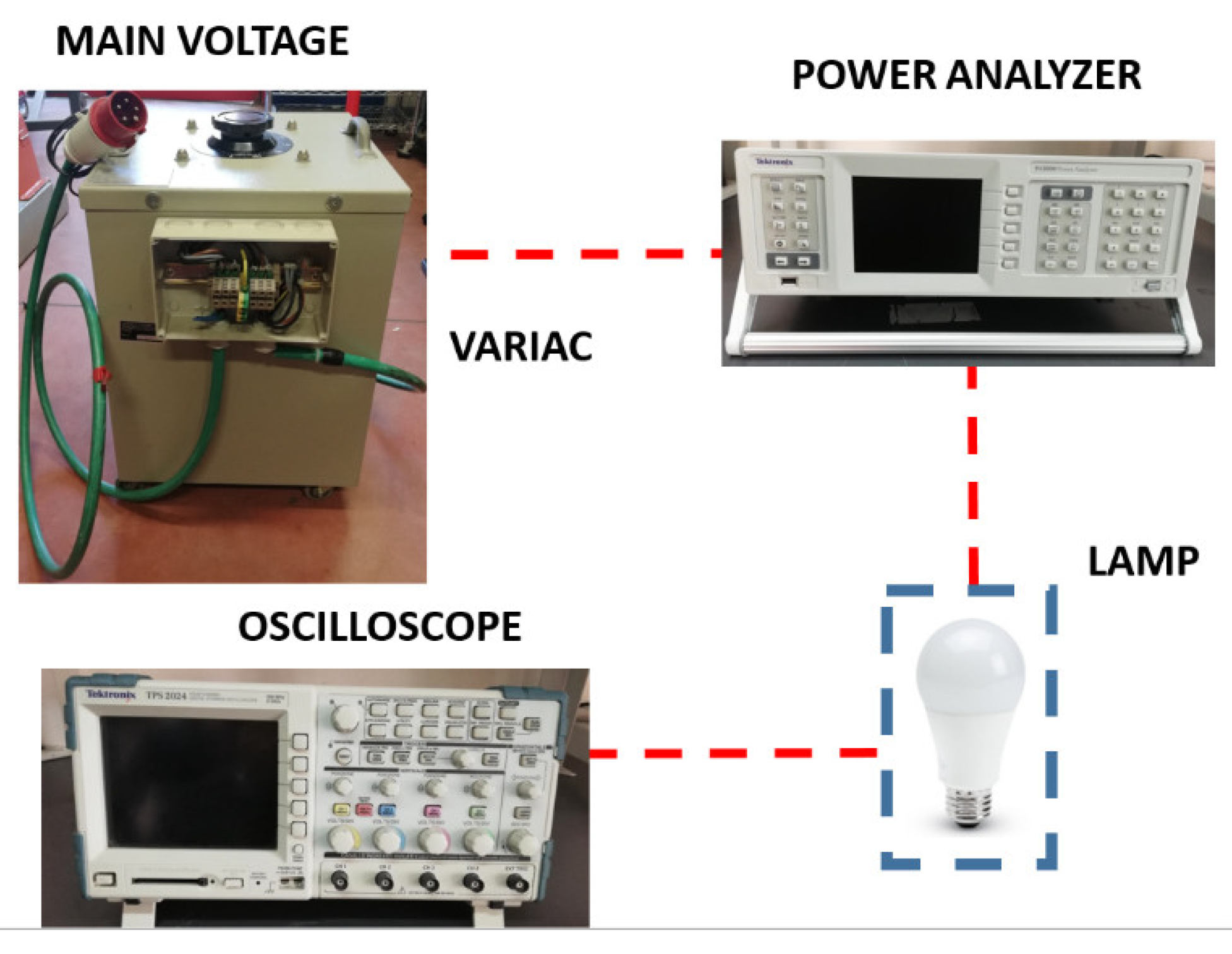
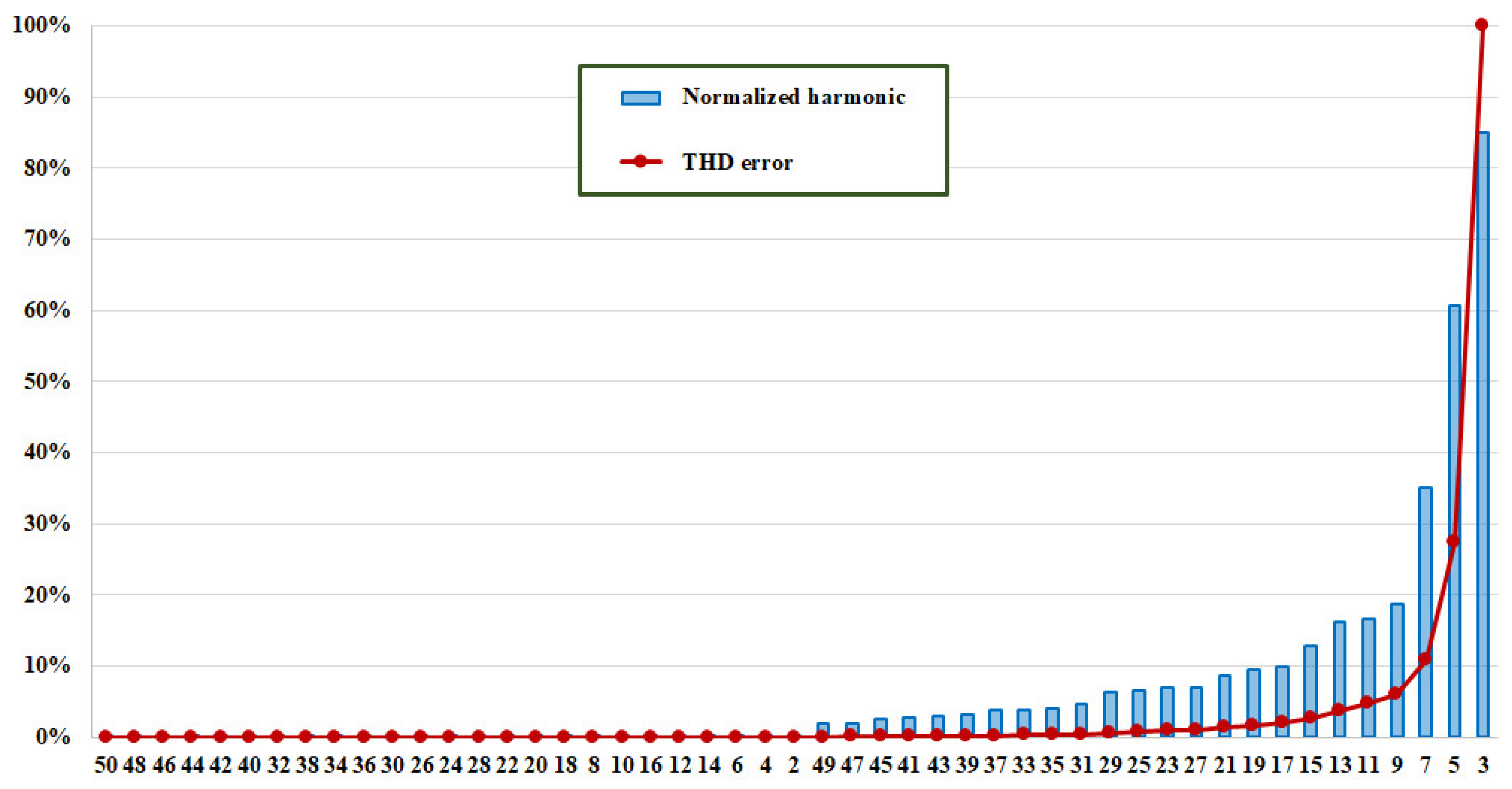


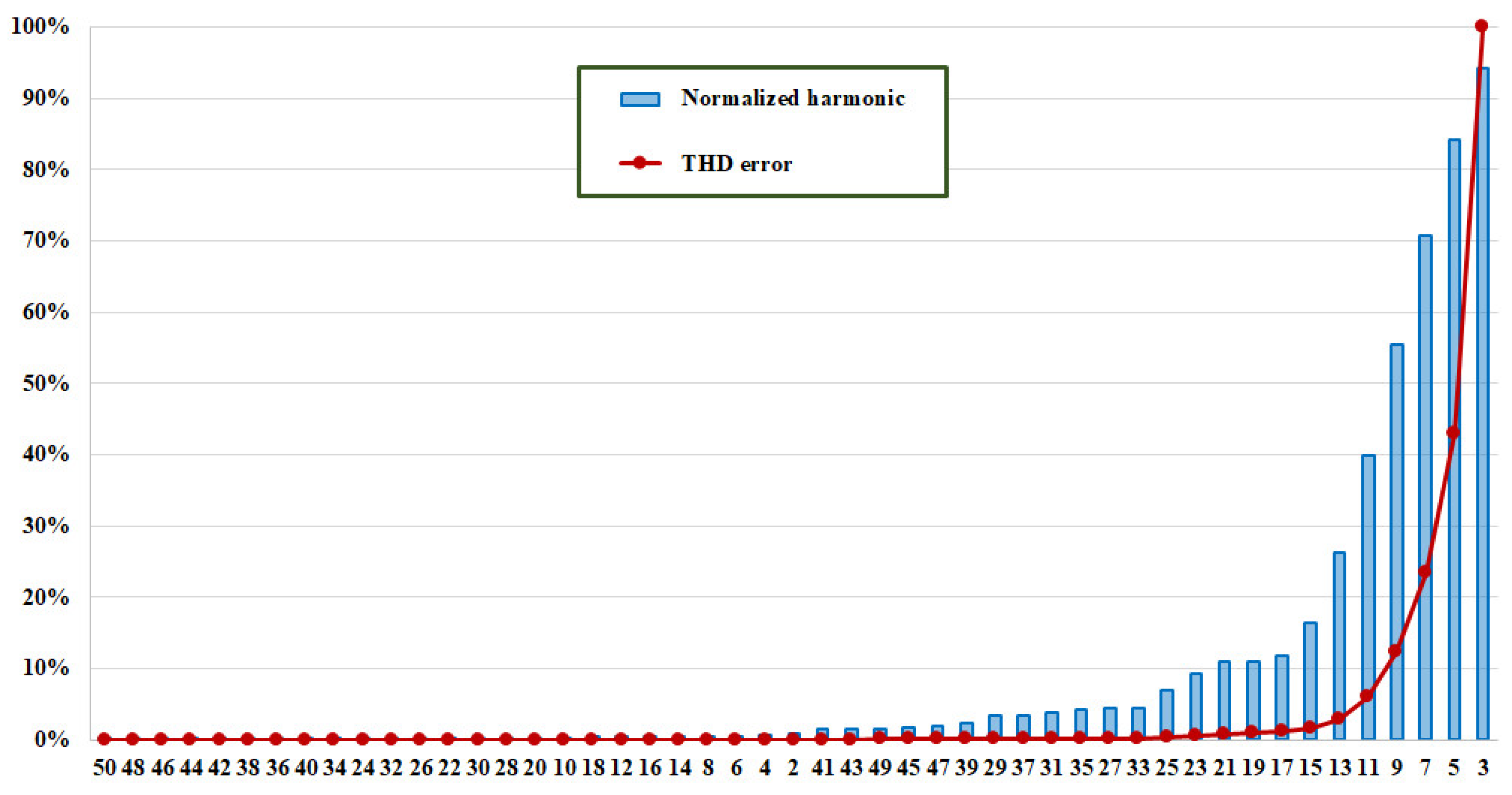
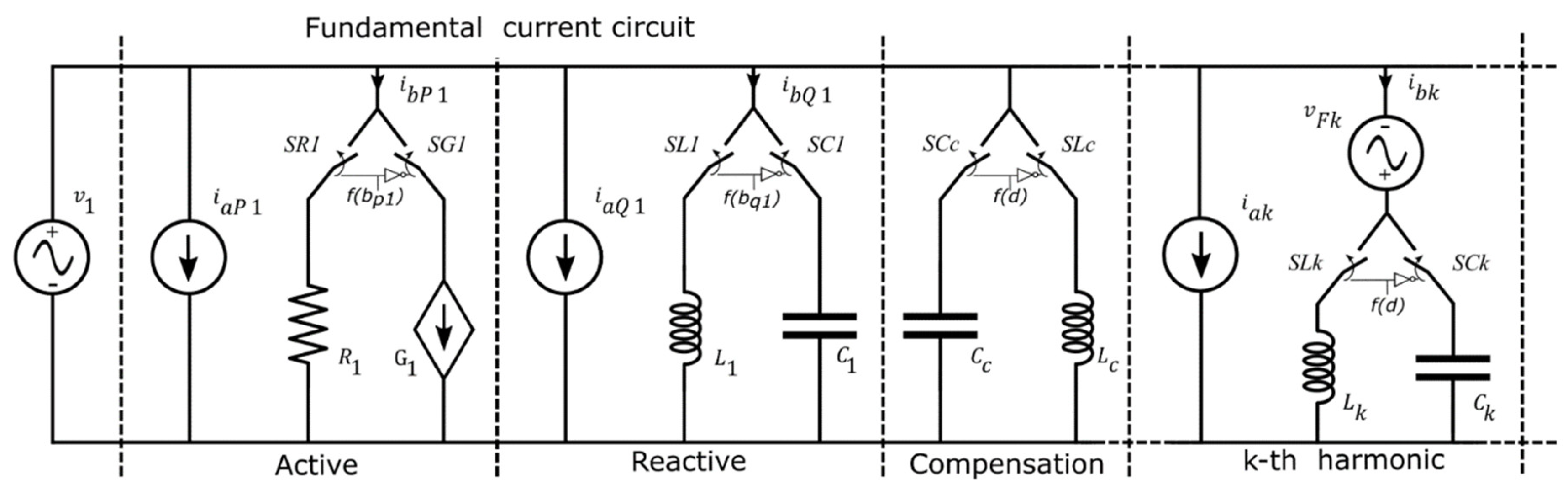
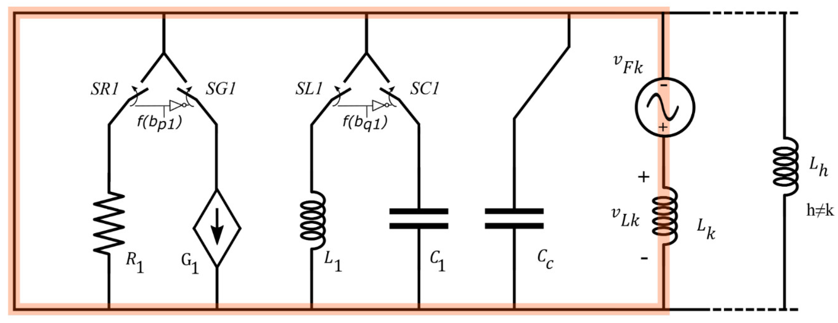
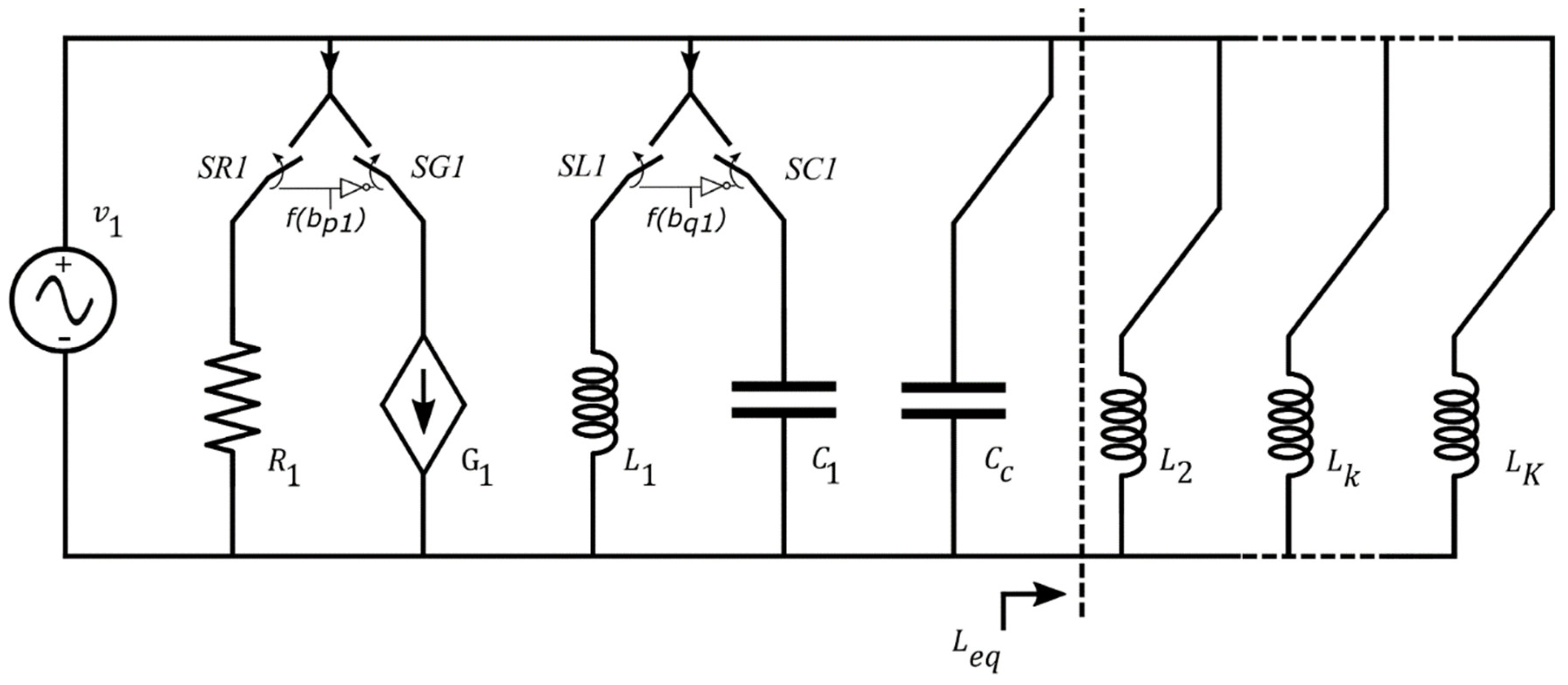
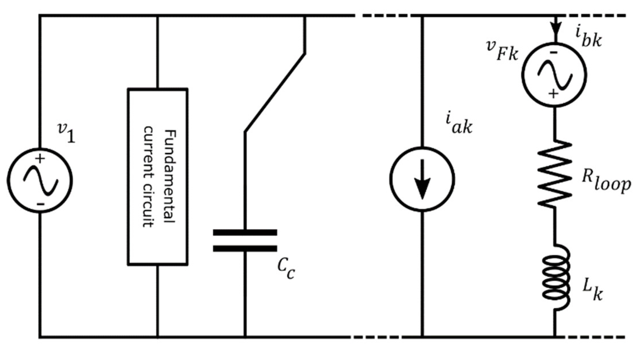
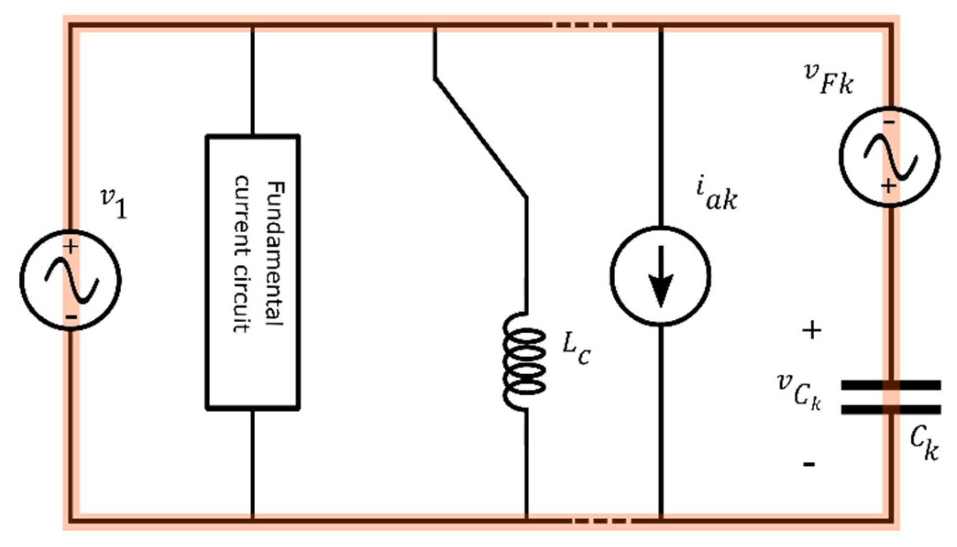

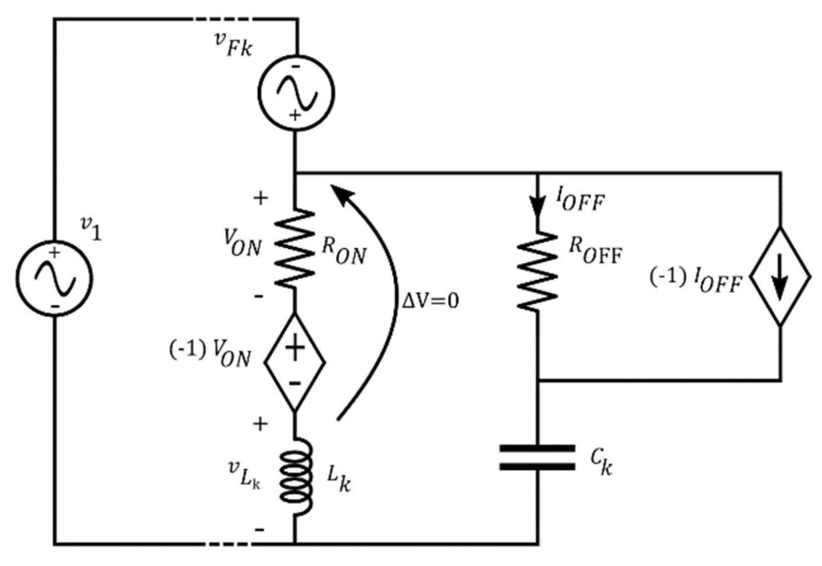
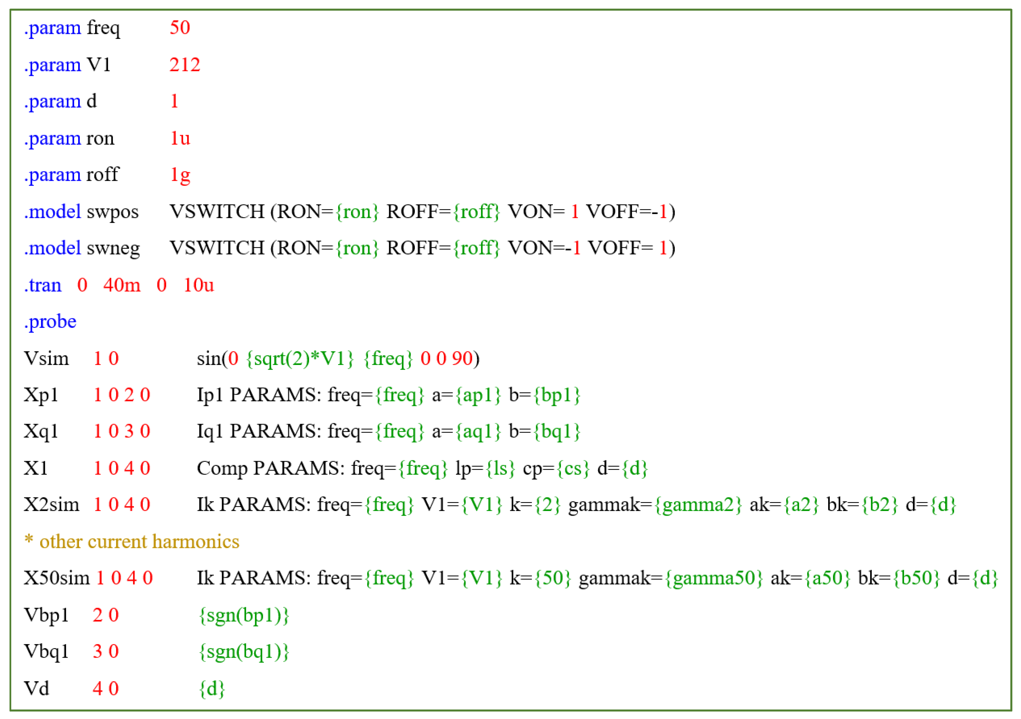
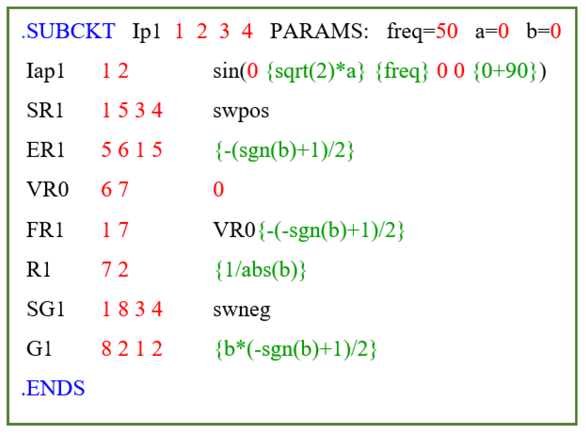
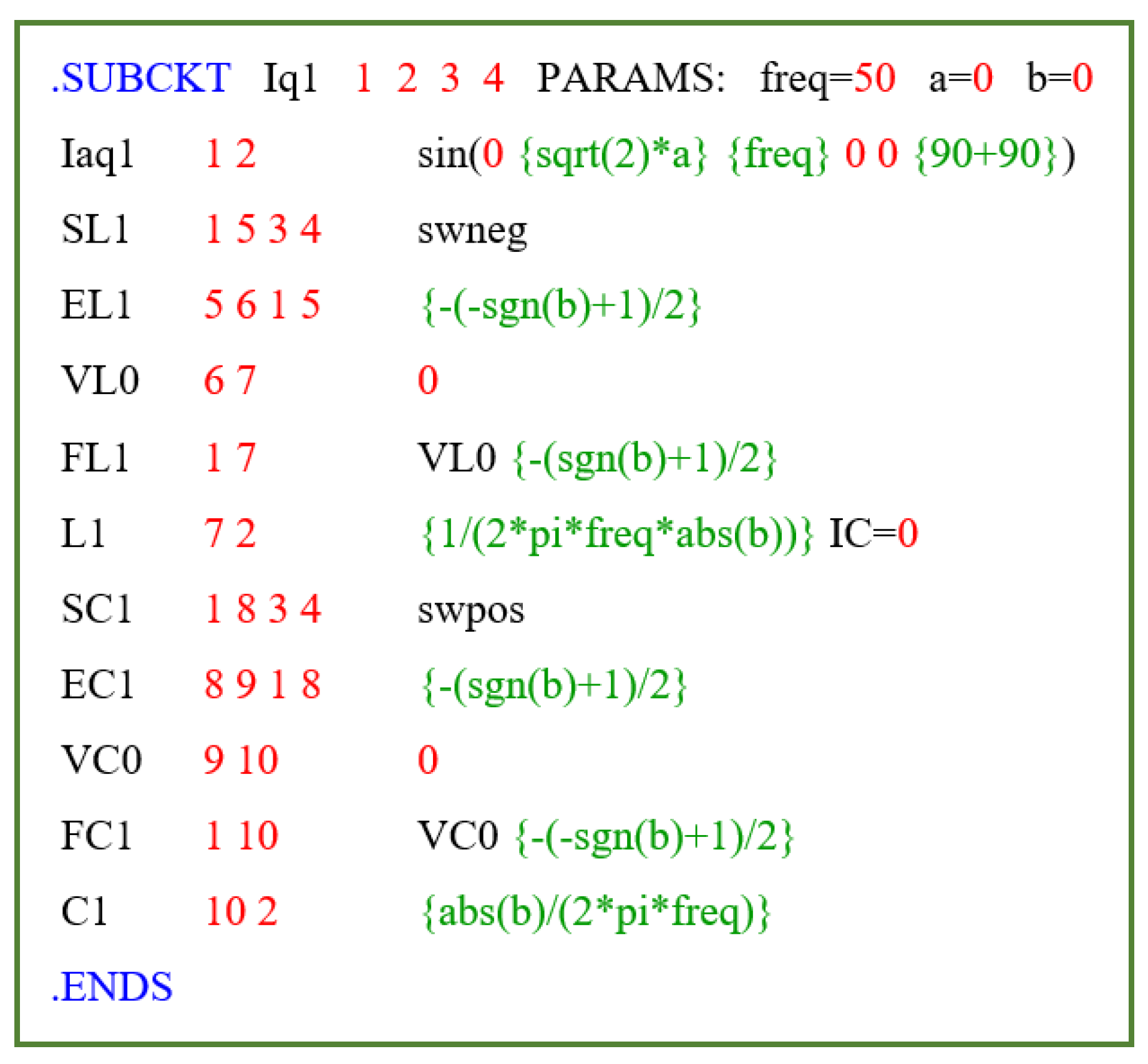
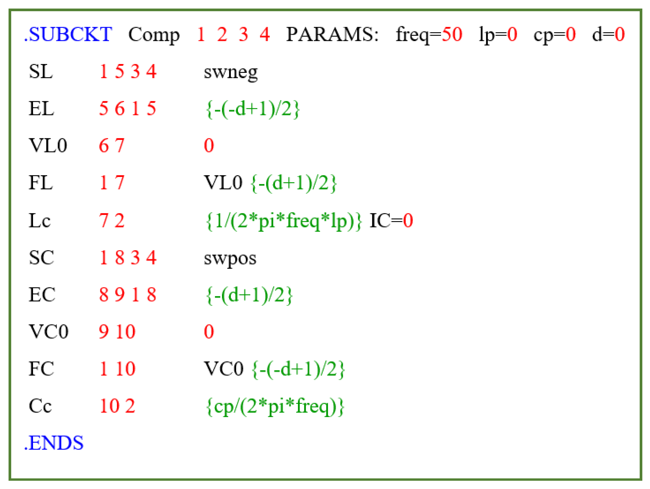
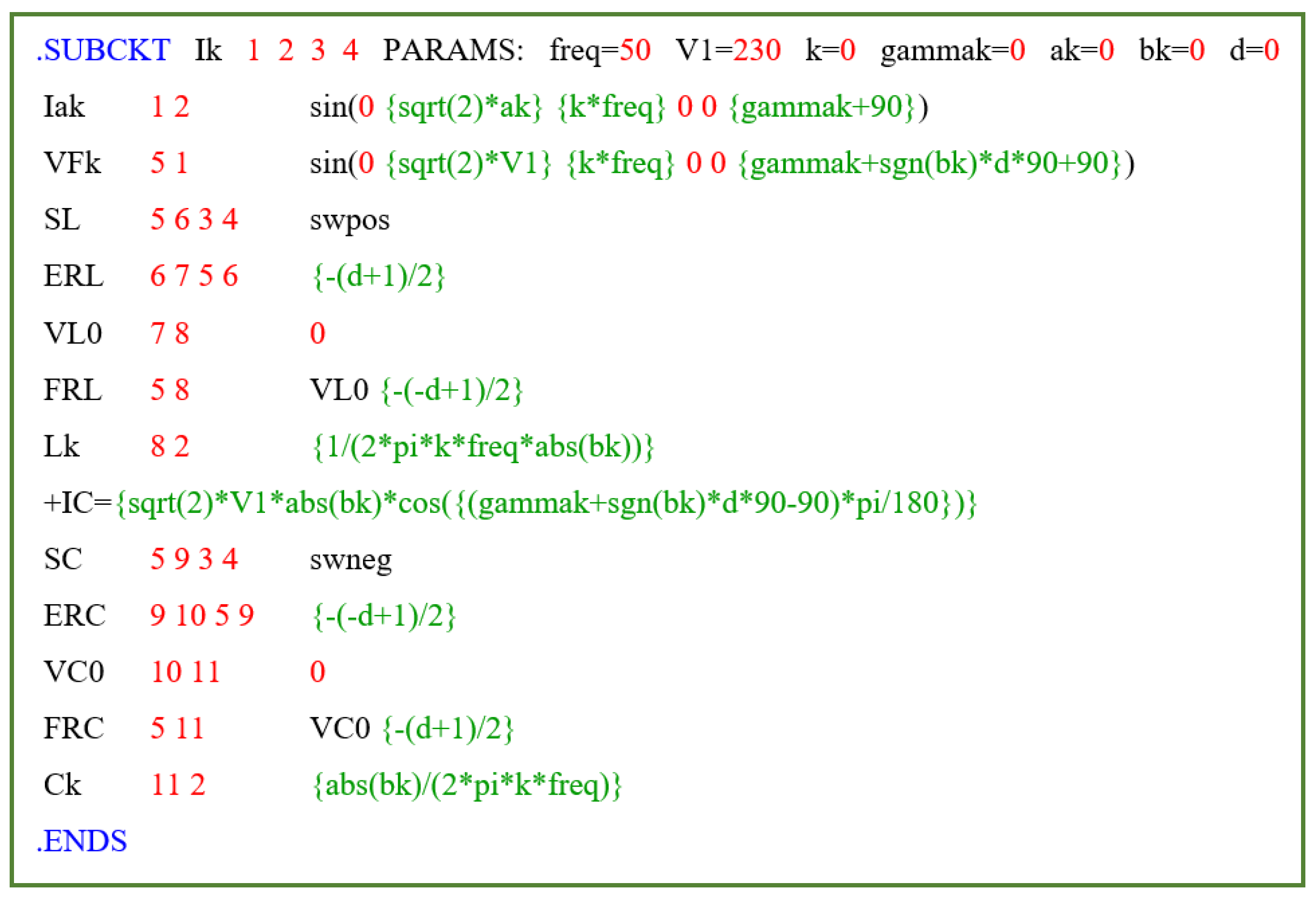

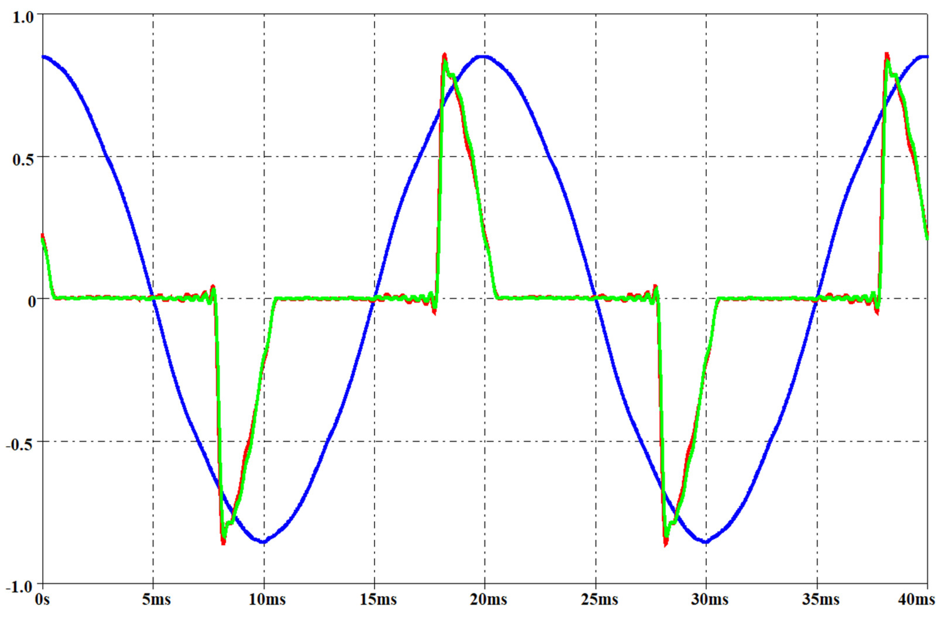
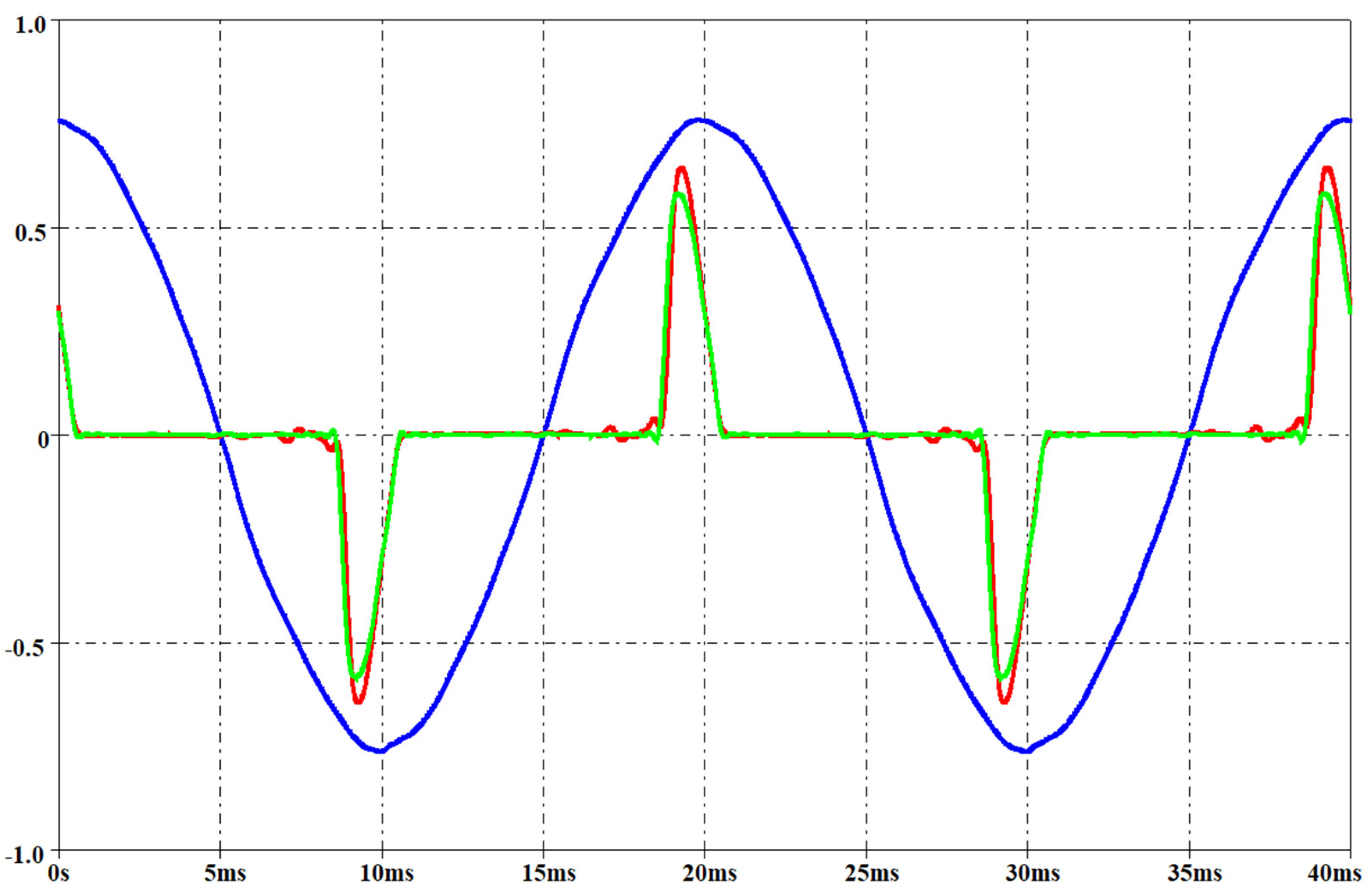

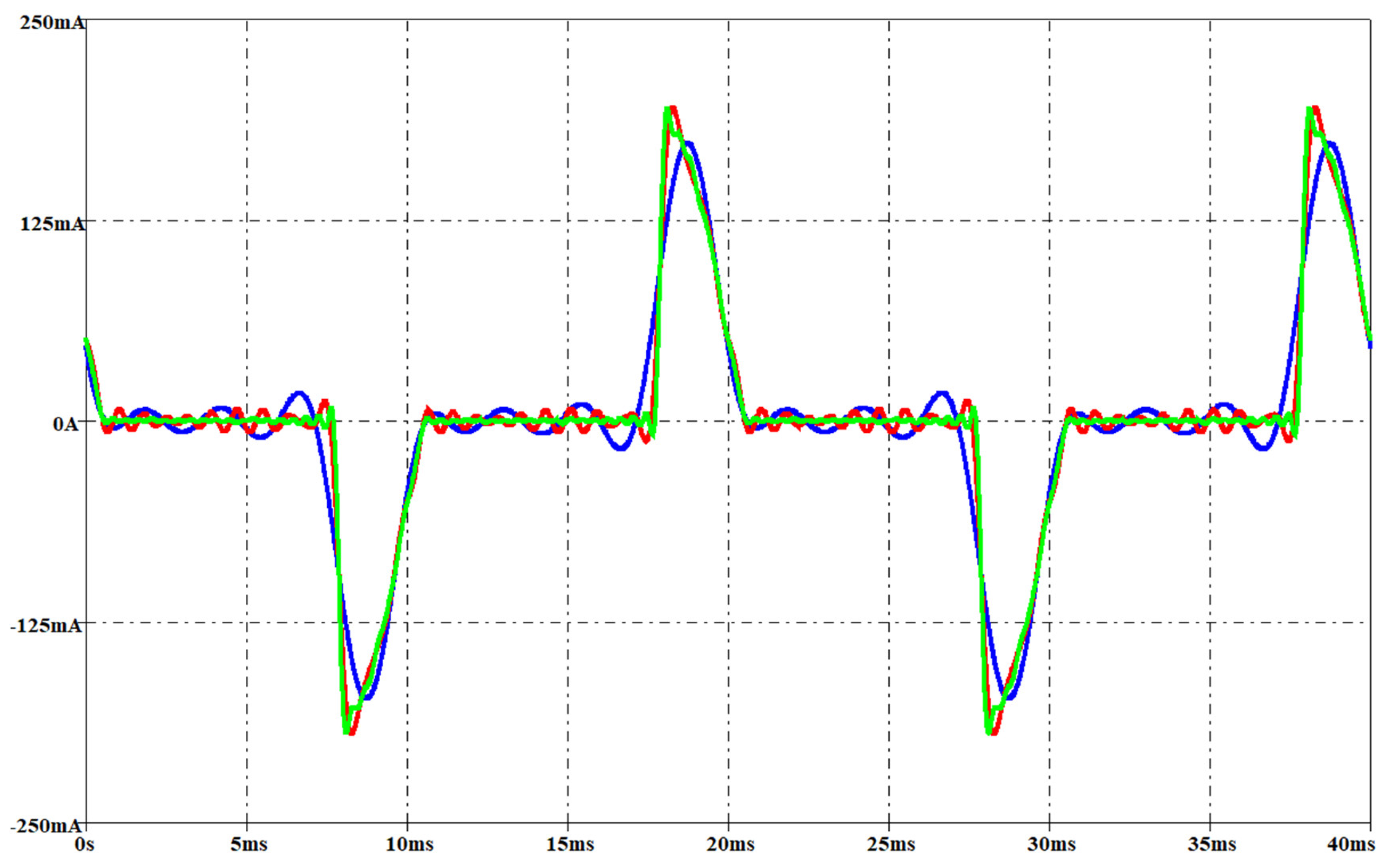
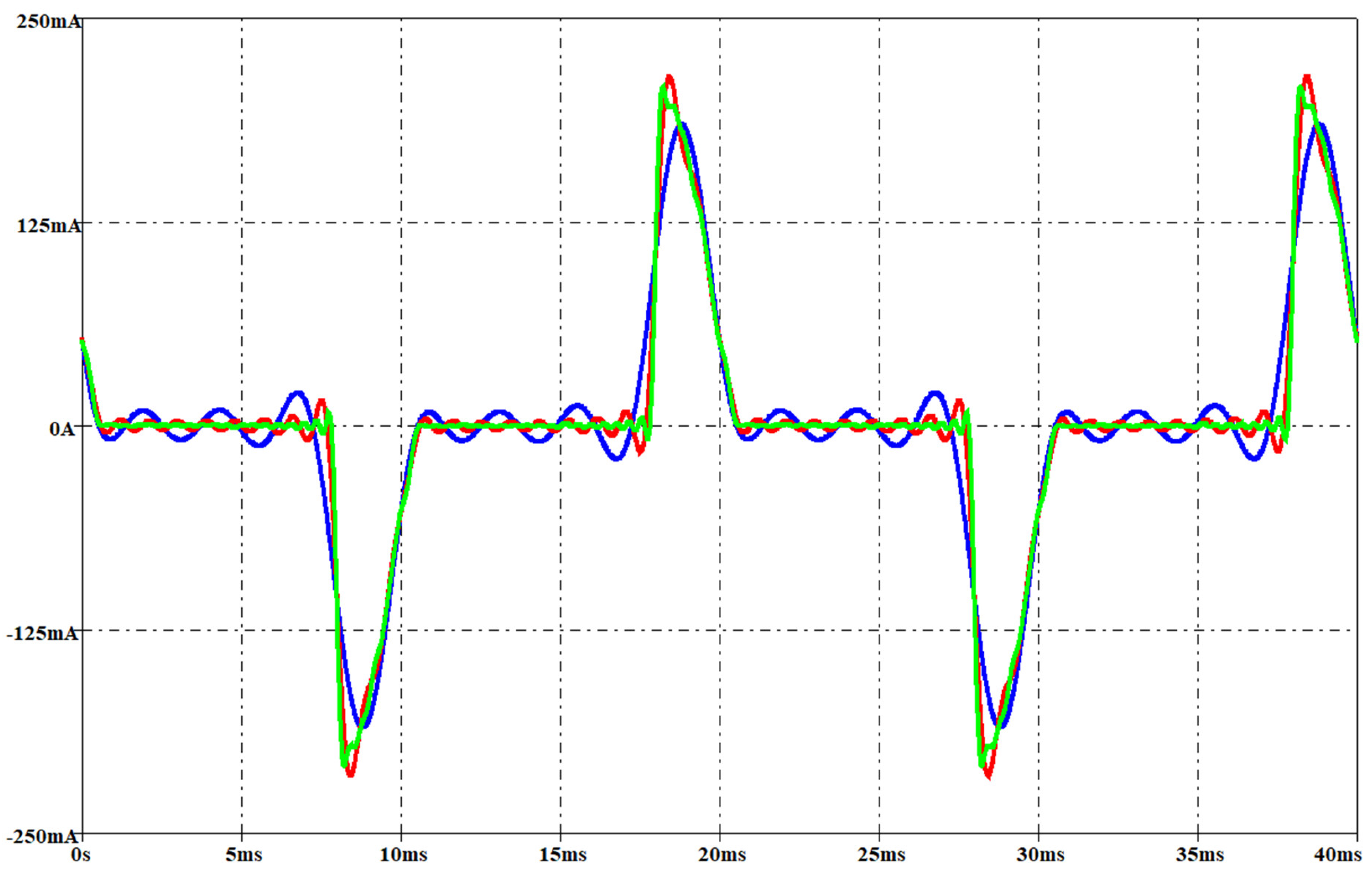
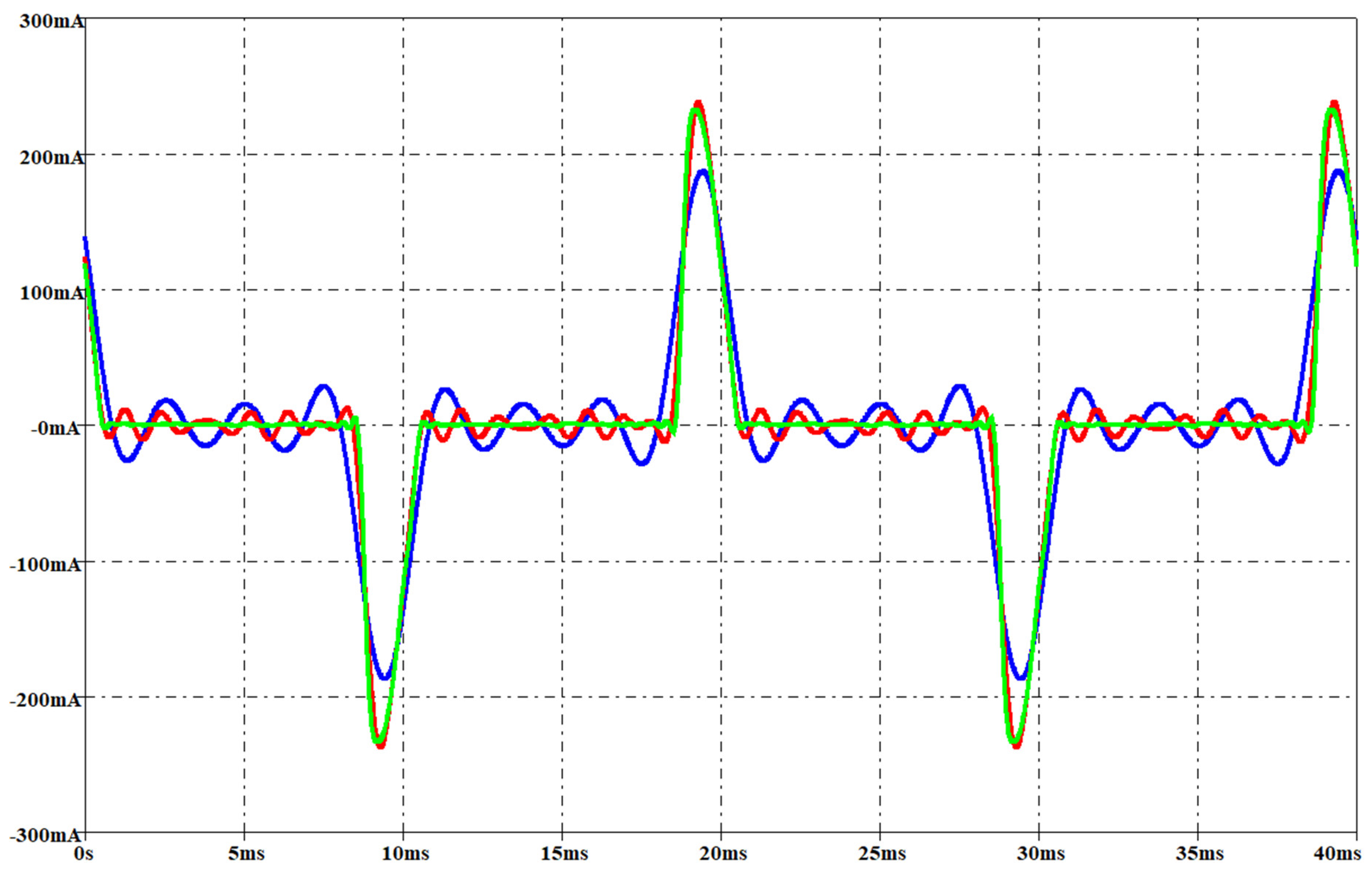
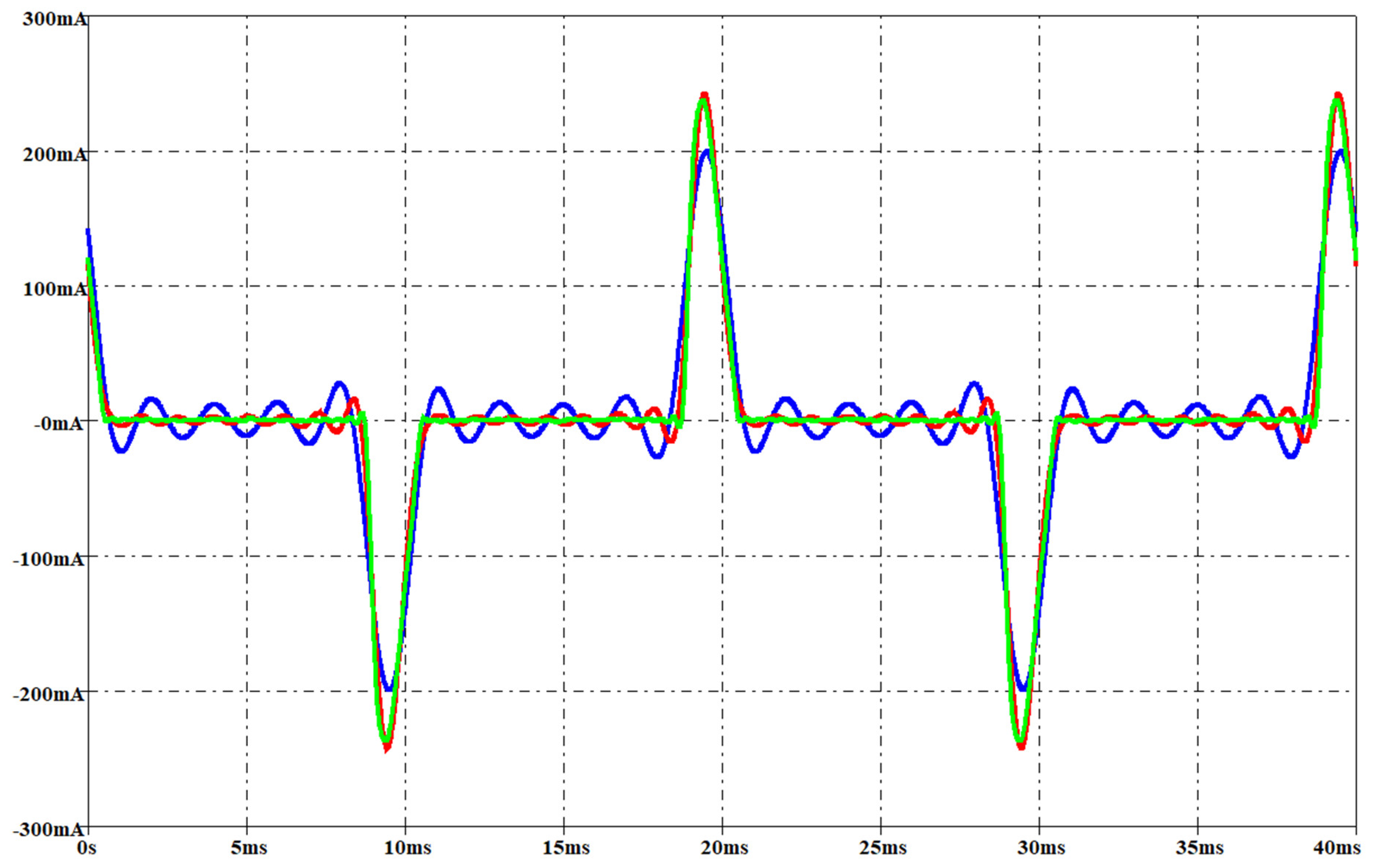
© 2019 by the authors. Licensee MDPI, Basel, Switzerland. This article is an open access article distributed under the terms and conditions of the Creative Commons Attribution (CC BY) license (http://creativecommons.org/licenses/by/4.0/).