Distributed Optimal Coordinated Operation for Distribution System with the Integration of Residential Microgrids

Abstract

With the increasing integration of rooftop photovoltaic (PV) generation and plug-in electric vehicles (EVs) into the households at user level, household consumers become prosumers. The coordination between the household prosumers and distribution network (DN) becomes essential to the energy management and optimal operation for both entities. In this paper, the residential prosumer cluster is considered as a residential microgrid (RMG) and a hierarchical DN integration method for the multi-RMGs is presented. A two-level hierarchical distributed optimization model is established based on the analytical target cascading to coordinate the RMGs and DNs. At the RMGs level, each RMG is required to individually optimize the energy consumption scheduling in every household by taking into account the effect of time-of-use electricity price on the demand response of EVs and flexible loads. At the DN level, the optimally coordinated operation problem is formulated as a relaxed optimal power flow model based on the second order cone programming by considering the power flow balance constraints. Case studies on the modified IEEE 33-bus system demonstrate the feasibility and effectiveness of the proposed method by achieving coordinated economic optimality as well as coordinated operating points for all entities.

1. Introduction

Present energy demands and greenhouse gas emissions have been promoting the rapid development of renewable-energy-based distributed generation and electric vehicles (EVs) [1]. With recent technological advancements, there has been a significant increment in integrating renewables and EVs into the end-user level. For instance, the presence of renewable distributed generation (e.g., PV generation at rooftops) and EVs in a residence or villa makes it function to supply its domestic loads by using the distributed energy resources (DERs). In this regard, residential end-users are facing the transition from consumers to prosumers, and the residential prosumers can be able to generate and consume energy internally looking for an autonomous operation [2]. The residential prosumers or prosumer clusters can be seen as residential microgrids (RMGs) with the capability to manage their distributed energy resources, e.g., renewable distributed generation units, EVs, flexible loads and their participation in demand response. As residential energy consumption occupies a considerable proportion of energy in the demand side [3,4], RMGs have attracted increasing concerns. In the near future, large numbers of RMGs may emerge prominently in active distribution networks (ADNs).

Considerable work has been undertaken concerning home/residential microgrid energy management for the integration of renewables and EVs into residential loads and optimization of energy consumption for end-users [5,6,7,8,9,10,11,12]. However, most of the existing literature is only directed toward a single residential microgrid system, the interaction relationship between RMGs and active distribution network (ADN) were not taken into account. In [5], an energy service decision-support tool is presented to schedule the available distributed energy resources integrated into the household to optimize home energy consumption and even provides energy services. In [6], an optimal management system is proposed for the energy management of a residential microgrid, this optimization model considered the renewable energy sources, integration of electric vehicles, vehicle to the grid system, and the energy consumption of a household with the day-ahead electricity price. The researchers in [9,10,11,12] studied the designing of home energy management systems for coordinated optimal control between the behavior of energy use of a household and the operation of distributed energy resources. In [13], optimal management problem of an RMG is formulated as a mixed integer linear programming model aiming for a minimum operating cost of the RMG, and its economic value is assessed from the perspective of a homeowner. In [14], an optimal energy management model for an RMG with various types of distributed energy sources is proposed; load scheduling potential of household appliances is taken into account. Optimal operation problems of RMGs in a given area are investigated in [15], based on local electricity prices and building characteristics, an optimization model is developed to minimize the electrical costs of all residential households in the RMG with associated constraints.

While the RMG and ADN are two different entities, they are actually also interconnected. The operating point of one entity impacts the operating point of the other. The energy management models presented in the literature mentioned above only considered supply–demand balance in single RMGs while ignoring the underlying ADN and the associated system operational and power flow constraints. The energy scheduling decisions are although beneficial for individual RMGs but they can threaten the distribution system efficiency. Therefore, coordination between RMGs and ADN is necessary and is of great importance. How to effectively coordinate the energy management and optimal operation between RMGs and ADN bring challenges for the residential microgrid owners (RMGOs) and distribution system operator (DSO). This paper focuses on a distributed coordinated method for optimal energy management and operation of RMGs integrated with ADN by considering the power flow and operational constraints.

In recent years, various distributed optimization methods such as, auxiliary problem principle, benders and optimality condition decomposition and alternating direction method of multipliers considering; energy management, dynamic economic dispatch and optimal power flow (OPF) problems have been studied extensively [16,17,18]. The distributed optimization methods are essentially iterative approaches based on decomposition–coordination. Compared with the traditional centralized method, the distributed method effectively decreases the model complexity and improves computational efficiency. Recently, the analytical target cascading (ATC) method (relatively new distributed algorithm) has been used and achieved satisfactory result in; unit commitment for multi-regional power systems [19], optimal operation problems of power system encompassing active distribution networks [20], collaborative optimal power flow (OPF) among the transmission system and active distribution grids [21]. Comparing with other distributed methods mentioned above, ATC method has more flexible coordination strategies with improved convergence properties [22]. However, the application of ATC method is fairly little in coordinating the operation of the distribution system and end-user level. In this paper, ATC method is extended to solve the optimally coordinated operation problems between the RMGs and ADN.

Moreover, residential demand response (DR) becomes increasingly attractive due to its great potential [23]. In [24], a residential DR management model is proposed to manage DR provided by flexible household loads, and it has been shown that the residential DR can reduce energy expense of individual households as well as flatten the total load profile of DN. However, EVs with DR potential were not taken into account. Emerging plug-in EVs in household prosumers and the associated Vehicle-to-Home (V2H) capability offer new residential DR resources for the RMG. Therefore, residential DR provided by EVs and V2H capability is incorporated in the modeling in this paper. To the best of the authors’ knowledge, there is no report about ATC-based distributed method applied to optimally coordinated operation problems between the RMGs and ADN that take into account residential DR and the underlying power flow and operational constraints on the ADN simultaneously.

In this paper, the cluster of household prosumers in the close spatial distance (e.g., residential district) is treated as an RMG and a hierarchical structure of ADN integration of multi-RMGs is presented. The RMGOs and DSO are regarded as two different entities with their autonomous objectives, ATC method is used to represent the collaboration and cooperation relationship between the RMGs and ADN. The energy management problem in RMG and optimal operation problem in ADN are modeled individually according to their own load demand and available energy sources The associated residential demand response and power flow balance is solved independently in a distributed coordination manner, and then the optimal coordinated operating point and economic benefit of each entity are achieved. A case study is conducted based on the modified IEEE-33 bus distribution system to verify the feasibility and effectiveness of the proposed method.

The remaining paper is organized as follows. The hierarchical structure of ADN integration of multi-RMGs is illustrated in Section 2. ATC-based distributed optimization modeling for RMGs and ADN is presented in Section 3. Section 3 illustrates the solving procedure. Section 4 shows the case studies and numerical results. Conclusions are drawn in Section 5.

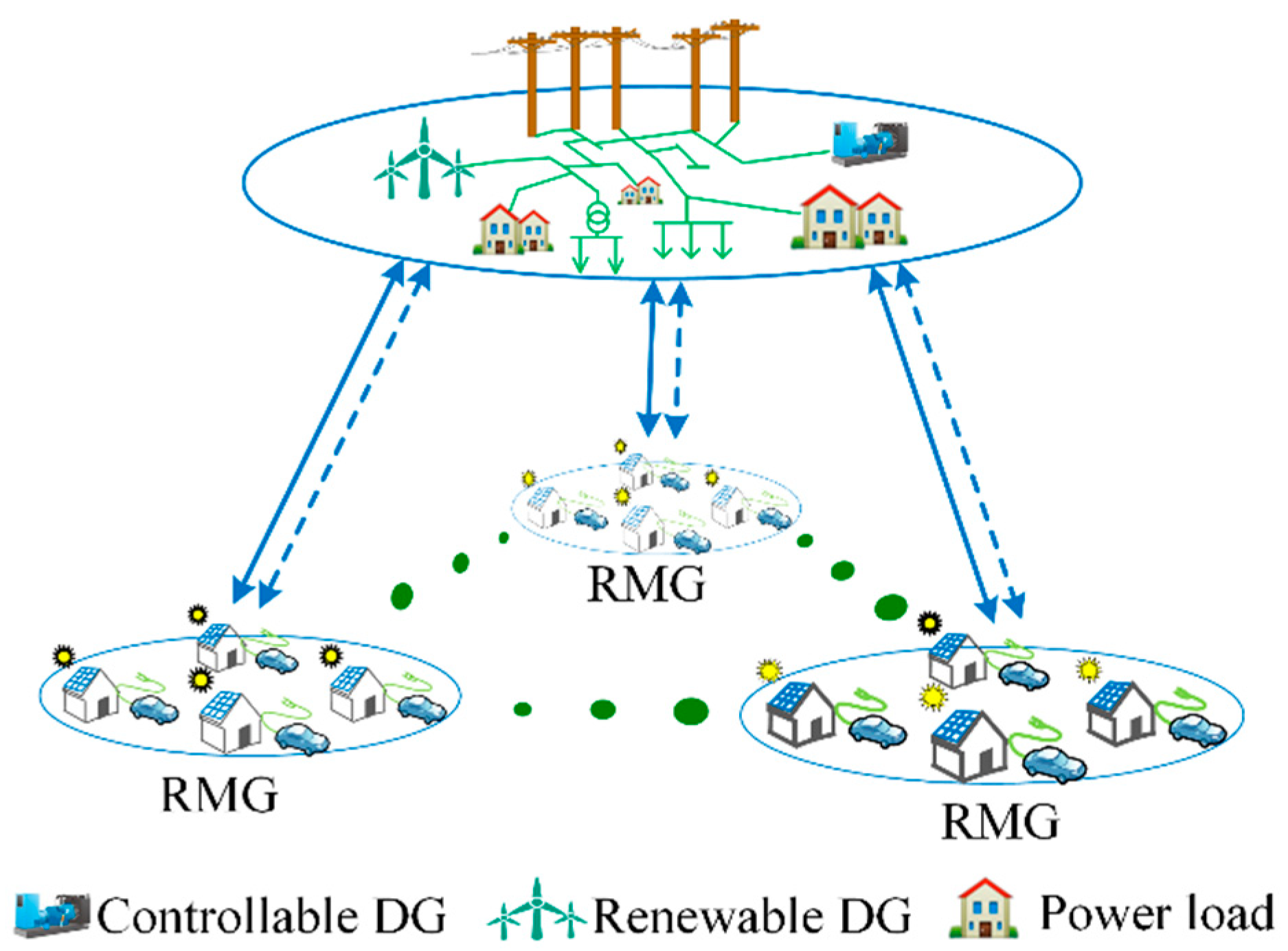
2. Description of Active Distribution Network Integration of Multi-RMGs

With the fast development of rooftop PV system and EVs, the households have local generation sources, such as the rooftop PV generation and plug-in electric vehicle battery energy storage, and thus are able to provide local energy production to supply their domestic power demand. That is, household prosumers can internally generate and consume energy, therefore, they are looking for autonomous operation. The households are usually located geographically close to each other [25], such as in the residential district, so the group of household prosumers are often collectively regarded as an RMG. The conceptual schematic outline of RMG is shown in Figure 1. The RMG is capable of operating both in an interactive and independent way. If there is electricity deficiency in RMG, RMG owners purchase electricity from DSO. If there is surplus power, the RMG is able to feed electricity back to the power distribution grid [26].

The hierarchical structure of ADN connected with multi-RMGs is illustrated in Figure 2. ADN is in the upper level and RMGs are in the lower level, two entities are linked together through tie-lines. In addition to a connection with the upstream grid, the ADN commonly consists of feeders, distributed generation (DG) (e.g., controllable DG, renewable DG, etc), and loads in a local region. As a new entity, the RMG has the ability to exchange power with the ADN and to communicate with the distribution system operator. It should be noted that the RMGs at the same level has no direct affiliation with each other.

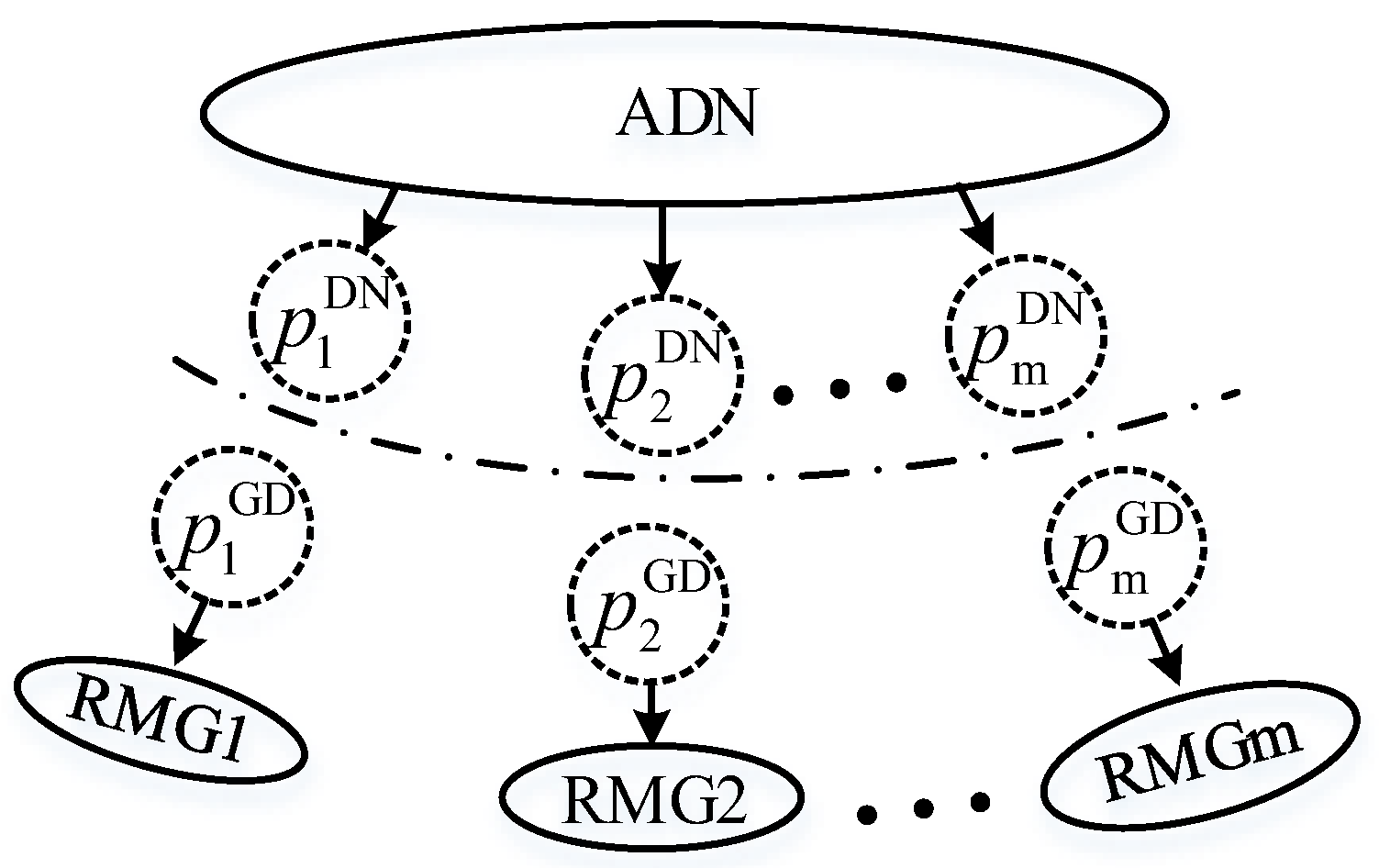
3. ATC-Based Distributed Modeling for Multi-RMGs Integrated in ADN

As different entities, the DSO and RMGO have different energy management objectives. The power flow in the tie-lines connecting the ADN and RMGs establishes the coupling operation between the two entities, and their energy management problems cannot be solved independently. A distributed method is required to coordinate the exchanged power in the tie-lines. The collaborative relationship between the ADN and RMGs can be represented by the analytical target cascading method.

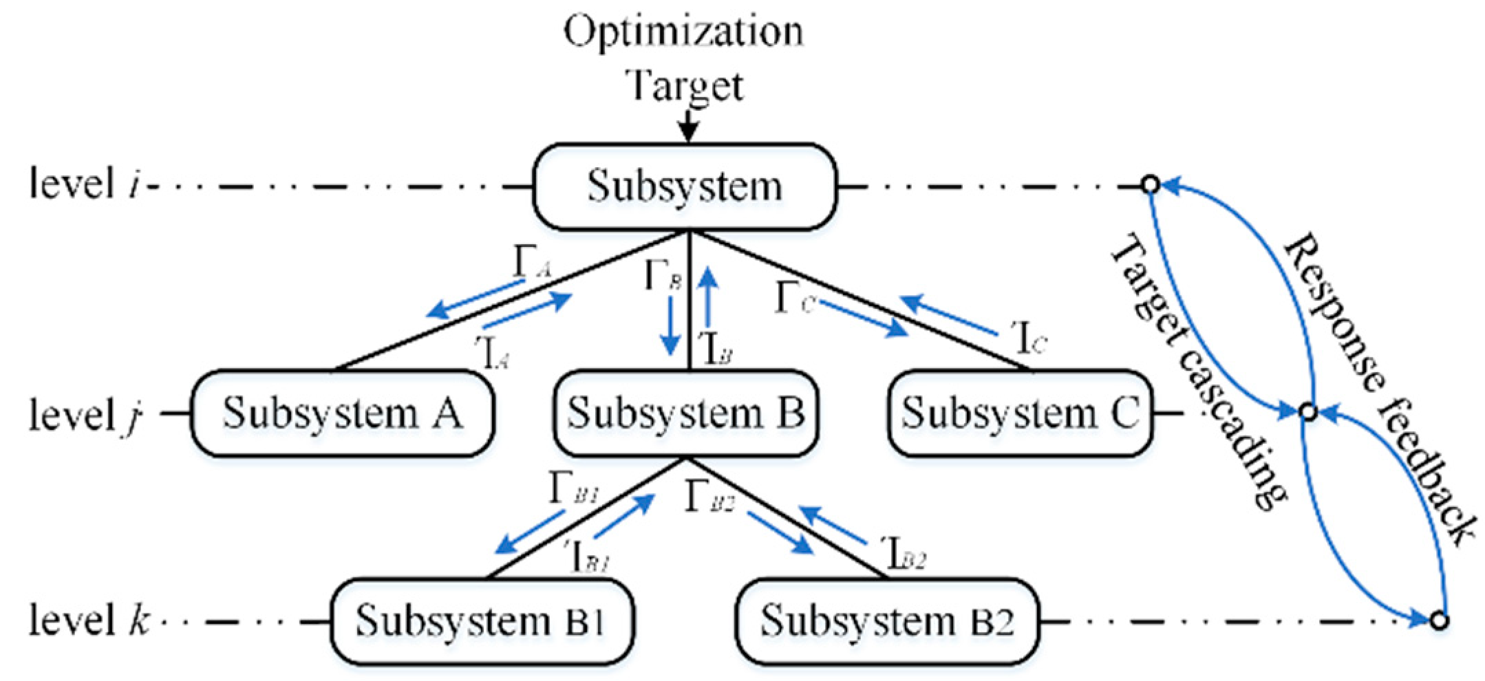
3.1. ATC-based Multilevel Hierarchical Optimization Mechanism

ATC is an effective and multi-level hierarchical optimization method for system design [27]. In the ATC method, the whole system is hierarchically partitioned into a series of individual subsystems. The subsystems from different levels are hierarchically linked, while the subsystems at the same level are not connected. Each subsystem has its own optimization sub-problem which can be independently solved. Moreover, the subsystems within the same level are solved in a parallel distributed fashion. So the whole complex optimization problem is transformed into an independent set of sub-problems, which significantly reduces the overall computation cost.

A three-level hierarchical ATC model is shown in Figure 3. A parent–child relationship is defined for the subsystems that have direct interdependencies. Subsystem in the upper-level is the parent of subsystems in the lower-level. By the same token, subsystems in the lower-level are the children of the subsystem in the upper-level. Targets (Γ) and responses (Ί) are shared variables that denote the linking relations between the parent and the children. A parent transfers the optimized target Γ to its child elements, and Γ becomes the matching objective of children’s responses Ί. In general, the simplified optimization model of the subsystem can be written as follows:

$$\min :f_{sub}+\pi \left(\Gamma -Ί\right)$$

(1)

$$\begin{array}{ll}\mathrm{s}.\mathrm{t}. & g_{sub}\le 0\\ & h_{sub}=0\end{array}$$

(2)

where $f_{sub}$ denotes the local optimization objective of the subsystem, $g_{sub}$ and $h_{sub}$ are the sets of inequality and equality constraints, $\pi \left(\Gamma -Ί\right)$ represents the penalty function added to a sub-problem aiming to minimize the deviation between parent target and child response. Note that except for the shared variables (Γ and Ί), the decision variables in the sub-problem are independent local variables in the sub-system. The introduction of penalty function enables (1) to be solved independently, and the shared variables are updated iteratively by solving the sub-problems. When $\Gamma -Ί$ = 0, i.e., the consistency constraint among the subsystems is reached, and the optimal solutions for the sub-problems can be achieved. And then, the final solution of the original complex optimization problem can be obtained. The advantage of the distributed algorithm is that it only requires limited information exchange among the parent and child elements during the optimization process.

The ATC characteristics described above are well-suited for the distributed nature of the RMGs and the hierarchical structure of ADN connected with Multi-RMGs. Therefore, the system as shown in Figure 2 can be partitioned into a two-level ATC hierarchy. The different entities (ADN and RMGs) are placed in different levels, and power flow in the tie-lines is a shared variable (i.e., coupling variable) among ADN and RMGs. In order to handle the couplings between the ADN and RMGs, the concept of virtual load and virtual generator is introduced to model the coupling variable as shown in Figure 4.

The tie-line power is equivalent to virtual load $p^{\mathrm{DN}}$ from the ADN standpoint and virtual generator $p^{\mathrm{GD}}$ from the RMG standpoint. Thus, $p^{\mathrm{GD}}$ is the power demanded by RMG and supplied by ADN in the RMG’s optimization problem; and $p^{\mathrm{DN}}$ is the power generated by ADN and supplied to RMG in AND’s optimization problem. According to the hierarchical optimization mechanism of ATC method, the consistency constraint (i.e., $p^{\mathrm{DN}}-p^{\mathrm{GD}}=0$) corresponding to every coupling variable needs to be enforced in RMG’s optimization sub-problem and ADN’s optimization sub-problem by using a penalty term. The penalty term added to sub-problem can be written as follows:

$$\{\begin{array}{ll}\pi (p^{\mathrm{DN}}-{\widehat{p}}^{GD})& \mathrm{added} \mathrm{to} \mathrm{ADN}’\mathrm{s} \text{sub-problem}\\ \pi (p^{\mathrm{GD}}-{\widehat{p}}^{DN})& \mathrm{added} \mathrm{to} \mathrm{RMG}’\mathrm{s} \text{sub-problem}\end{array}$$

(3)

where ${\widehat{p}}^{GD}$ is the prescheduled value for the virtual generator received from the RMGs, ${\widehat{p}}^{DN}$ is the prescheduled value for the virtual load received from the ADN. That is, while ${\widehat{p}}^{GD}$ is constant in the ADN’s optimization sub-problem, ${\widehat{p}}^{DN}$ is constant in the RMGs’ optimization sub-problems. There are several options to construct the penalty term $\pi (·)$, such as exponential penalty function, quadratic penalty function and augmented Lagrange penalty function. Compared to the first two penalty functions, the last one has better convergence property [28]. Thus, the augmented Lagrange penalty function is adopted in this paper.

Based on the above measures, the optimal operation problems of ADN and RMGs are completely separated from each other, which can be modeled and solved independently.

3.2. Optimization Model for RMG

The RMG considered in this work corresponds to a cluster of household prosumers, therefore the main purpose of this paper is to promote the local consumption of energy generated by the DERs rather than exporting the surplus power to the distribution system. It is assumed that every household contains PV generator, EV, flexible loads (i.e., shiftable load and adjustable load), and inflexible loads. The optimization objective aims to minimize the total energy consumption cost within mth RMG during the dispatching time period (e.g., 24 h) by taking into account the demand response of EVs and shiftable loads. The optimization model of the mth RMG within the ATC framework can be formulated as follows

$$\min :F_{RMGm}+{\displaystyle \sum _{t=1}^T\pi (p_{m,t}^{\mathrm{GD}}-{\widehat{p}}_{m,t}^{DN})}$$

(4)

$$F_{RMGm}={\displaystyle \sum _{t=1}^T{\displaystyle \sum _{h=1}^H{\lambda }_t(P_{h,t}^{\mathrm{infl}}+}}{\tau }_{h,t}^{\mathrm{ch}}{P}_{h,t}^{\mathrm{EV}\_\mathrm{ch}}-{\tau }_{h,t}^{\mathrm{dis}}{P}_{h,t}^{\mathrm{EV}\_\mathrm{dis}}+{\displaystyle \sum _{k=1}^{N_{fl}}{\mu }_{h,k,t}{P}_{h,k,t}^{\mathrm{fl}}}-P_{h,t}^{\mathrm{PV}})$$

(5)

In the above formulation, the objective function (4) consists of local optimization objective (5) of the mth RMG as well as its penalty function $\pi (·)$. In function (5), $P_{h,t}^{\mathrm{infl}}$ represents the power demand for inflexible load within hth household at hour t. $P_{h,k,t}^{\mathrm{fl}}$ represents the power demand of flexible load k within hth household at hour t. $P_{h,t}^{\mathrm{EV}\_\mathrm{ch}}$ and $P_{h,t}^{\mathrm{EV}\_\mathrm{dis}}$ respectively represent the charging and discharging power of the EV within hth household at hour t. $P_{h,t}^{\mathrm{PV}}$ represents the power output of the PV generator within hth household at hour t. ${\lambda }_t$ represents the electricity price at hour t. ${\mu }_{h,k,t}^{}$ represents the demand response coefficient of flexible load k within hth household, ${\mu }_{h,k,t}^{}$ is a binary variable, where 1 denotes flexible load k put into operation at hour t. ${\tau }_{h,t}^{\mathrm{ch}}$ is binary variable, where 1 indicates charging state of the EV within hth household at hour t. ${\tau }_{h,t}^{\mathrm{dis}}$ is binary variable, where 1 denotes discharging state of the EV within hth household at hour t.

The above optimization problem is subject to the following constraints.

(1)

EV load constraints

$${\tau }_{h,t}^{ch}+{\tau }_{h,t}^{dis}\le 1$$

(6)

$${\tau }_{h,t}^{\mathrm{ch}}{P}_{h,t}^{\min \_\mathrm{ch}}\le P_{h,t}^{\mathrm{EV}\_\mathrm{ch}}\le {\tau }_{h,t}^{\mathrm{ch}}{P}_{h,t}^{\max \_\mathrm{ch}}$$

(7)

$${\tau }_{h,t}^{\mathrm{dis}}{P}_{h,t}^{\min \_\mathrm{dis}}\le P_{h,t}^{\mathrm{EV}\_\mathrm{dis}}\le {\tau }_{h,t}^{\mathrm{dis}}{P}_{h,t}^{\max \_\mathrm{dis}}$$

(8)

$$E_h^{\mathrm{EV}\_\min }\le E_{h,t}^{\mathrm{EV}}\le E_h^{\mathrm{EV}\_\max }$$

(9)

$$E_{h,t}^{\mathrm{EV}}=E_{h,t-1}^{\mathrm{EV}}-E_{h,t}^{\mathrm{EV}\_\mathrm{Dri}}+{\eta }_h^{\mathrm{ch}}{P}_{h,t}^{\mathrm{EV}\_\mathrm{ch}}-\frac{1}{{\eta }_h^{\mathrm{dis}}}{P}_{h,t}^{\mathrm{EV}\_\mathrm{dis}}$$

(10)

Constraint (6) describes that a single EV cannot be in charging and discharging state simultaneously. Constraints (7) and (8) denote the minimum and maximum charging/discharging power limits. Constraint (9) limits the minimum and maximum allowable state-of-energy values of the EV. Constraint (10) shows energy stored in the EV in the current time period, which is associated with the energy remaining in the EV in the previous time period. The energy consumed during outdoor driving or the change in the amount of power generated through charging and discharging in the current time period.

(2)

Shiftable load constraints

$$0\le {\displaystyle \sum _{k=1}^{N_{fl}}{P}_{h,k,t}^{\mathrm{fl}}}{\mu }_{h,k,t}^{}\le P_h^{\mathrm{DR}\_\max }$$

(11)

$${\displaystyle \sum _{t=1}^{T-t_{op,k}+1}{\mu }_{k,t}=1}$$

(12)

$${\displaystyle \sum _{\ell =1}^{t_{op,k}}(1-{\mu }_{k,t-\ell +1})=0}$$

(13)

Constraint (11) denotes the shiftable load power limit. Constraint (12) guarantees that each shiftable load, i.e., shiftable household appliance can be scheduled just once over a 24-h time span. Constraint (13) ensures a continuous power supply during the working cycle of the appliance load, t_op,k denotes the working cycle of appliance load (h).

(3)

Rooftop PV power limit

$$P_h^{\mathrm{PV}\_\min }\le P_{h,t}^{\mathrm{PV}}\le P_h^{\mathrm{PV}\_\max }$$

(14)

(4)

Virtual generator power constraint

$$p_m^{\mathrm{GD}\_\min }\le p_{m,t}^{\mathrm{GD}}\le p_m^{\mathrm{GD}\_\max }$$

(15)

(5)

Supply–demand balance in RMG

$$p_{m,t}^{\mathrm{GD}}+P_{h,t}^{\mathrm{PV}}+{\tau }_{h,t}^{\mathrm{dis}}{P}_{h,t}^{\mathrm{EV}\_\mathrm{dis}}=P_{h,t}^{\mathrm{infl}}+{\displaystyle \sum _{k=1}^{N_{fl}}{\mu }_{h,k,t}{P}_{h,k,t}^{\mathrm{fl}}}$$

(16)

3.3. Optimization Model for ADN

The general optimization problem of a DN within the ATC framework can be formulated as follows:

$$\min :F_{ADN}+{\displaystyle \sum _{t=1}^T}{\displaystyle \sum _{m=1}^{N_{RMG}}\pi (p_{m,t}^{\mathrm{DN}}-{\widehat{p}}_{m,t}^{GD})}$$

(17)

$$F_{ADN}={\displaystyle \sum _{t=1}^T[C^{\mathrm{G}}{P}_t^{\mathrm{G}}+{\displaystyle \sum _{l=1}^{N_{bus}-1}{C}^{\mathrm{G}}{P}_{l,t}^{\mathrm{loss}}+{\displaystyle \sum _{g=1}^{N_{DG}}{C}^{\mathrm{DG}}{P}_{g,t}^{\mathrm{DG}}]}}}$$

(18)

In the above formulation, the objective function (17) consists of local optimization objective (18) of the ADN as well as its penalty functions. In the local optimization objective (18), the first item represents the cost of buying electricity from the upstream grid in tth hour, where $C^{\mathrm{G}}$ represents the price for purchasing electricity from the upstream grid ($/kW), $P_t^{\mathrm{G}}$ represents the power transferred from the upstream grid to the ADN (kW). The second item represents the power loss cost of ADN, where $P_{l,t}^{\mathrm{loss}}$ represents the power loss of lth branch of the ADN in tth hour. The third item is the generation costs of all controllable DGs in the ADN, where $C^{\mathrm{DG}}$ represents generation cost of controllable DG, $P_{g,t}^{\mathrm{DG}}$ represents the power output of the gth DG at the hour t.

The above optimization problem is subject to the following constraints:

(1)

Power balance constraint

$$\{\begin{array}{l}{P}_t^{\mathrm{G}}+{\displaystyle \sum _{g=1}^{N_{DG}}{P}_{g,t}^{\mathrm{DG}}}-{\displaystyle \sum _{l=1}^{N_{bus}-1}{P}_{l,t}^{\mathrm{loss}}}=P_t^{\mathrm{D}}+{\displaystyle \sum _{m=1}^M{p}_{m,t}^{\mathrm{DN}}}\\ {\displaystyle \sum _{l=1}^{N_{bus}-1}{P}_{l,t}^{\mathrm{loss}}}={\displaystyle \sum _{l=1}^{N_{bus}-1}{r}_l{I}_{l,t}^2}\end{array}$$

(19)

(2)

Constraint of power transferred from the upstream grid

$$0\le P_t^{\mathrm{G}}\le P_t^{\mathrm{G}\_\max }$$

(20)

(3)

DG output power constraint

$$P_{g,t}^{\mathrm{DG}\_\min }\le P_{g,t}^{\mathrm{DG}}\le P_{g,t}^{\mathrm{DG}\_\max }$$

(21)

(4)

Virtual load power constraint

$$p_m^{\mathrm{DN}\_\min }\le p_{m,t}^{\mathrm{DN}}\le p_m^{\mathrm{DN}\_\max }$$

(22)

Note that the optimization model of ADN is a nonlinear nonconvex programming problem which is difficult to solve, and the convergence and optimality of solutions cannot be ensured in the ATC framework [28]. The optimization problem of ADN can be regarded as an OPF problem when the power flow balance constraints are taken into account [29]. The optimization model of ADN can be transformed into a second order convex programming (SOCP) problem based on a relaxed DistFlow model [30]. The power flow balance in the ADN can be described as a quadratic model based on DistFlow:

$$\begin{array}{l}{\displaystyle \sum _{k\in \mathsf{\Omega }(j)}{P}_{jk,t}}-{\displaystyle \sum _{i\in \mathsf{\Psi }(j)}(P_{ij,t}}-r_{ij}{I}_{ij,t}^2)=P_{j,t}^{\mathrm{G}}+P_{j,t}^{\mathrm{DG}}-P_{j,t}^{\mathrm{d}}-P_{j,t}^{\mathrm{DN}}\\ {\displaystyle \sum _{k\in \mathsf{\Omega }(j)}{Q}_{jk,t}}-{\displaystyle \sum _{i\in \mathsf{\Psi }(j)}(Q_{ij,t}}-x_{ij}{I}_{ij,t}^2)=Q_{j,t}^{\mathrm{G}}+Q_{j,t}^{DG}-Q_{j,t}^{\mathrm{d}}-Q_{j,t}^{DN}\end{array}$$

(23)

$$V_{j,t}^2=V_{i,t}^2-2(P_{ij,t}{r}_{ij}+Q_{ij,t}{x}_{ij})+I_{ij,t}^2(r_{ij}^2+x_{ij}^2)$$

(24)

According to [30], the second order cone equation can be obtained after relaxing the original quadratic model.

$$\begin{array}{l}{\displaystyle \sum _{k\in \mathsf{\Omega }(j)}{P}_{jk,t}}-{\displaystyle \sum _{i\in \mathsf{\Psi }(j)}(P_{ij,t}}-r_{ij}{\tilde{I}}_{ij,t})=P_{j,t}^{\mathrm{G}}+P_{j,t}^{\mathrm{DG}}-P_{j,t}^{\mathrm{d}}-P_{j,t}^{\mathrm{DN}}\\ {\displaystyle \sum _{k\in \mathsf{\Omega }(j)}{Q}_{jk,t}}-{\displaystyle \sum _{i\in \mathsf{\Psi }(j)}(Q_{ij,t}}-x_{ij}{\tilde{I}}_{ij,t})=Q_{j,t}^{\mathrm{G}}+Q_{j,t}^{\mathrm{DG}}-Q_{j,t}^{\mathrm{d}}-Q_{j,t}^{\mathrm{DN}}\end{array}$$

(25)

$${\tilde{V}}_{j,t}={\tilde{V}}_{i,t}-2(P_{ij,t}{r}_{ij}+Q_{ij,t}{x}_{ij})+{\tilde{I}}_{ij,t}(r_{ij}^2+x_{ij}^2)$$

(26)

$${\Vert \begin{array}{l}2P_{ij,t}\\ 2Q_{ij,t}\\ {\tilde{I}}_{ij,t}-{\tilde{V}}_{i,t}\end{array}\Vert }_2\le {\tilde{I}}_{ij,t}+{\tilde{V}}_{i,t}$$

(27)

And subject to the following security constraints:

$$\begin{array}{l}{(V_j^{\min })}^2\le {\tilde{V}}_{j,t}\le {(V_j^{\max })}^2\\ 0\le {\tilde{I}}_{ij,t}\le {(I_{ij}^{\max })}^2\end{array}$$

(28)

Thus, the optimization problem of ADN can be reformulated as:

$$\begin{array}{l}\min :{\displaystyle \sum _{t=1}^T[C^{\mathrm{G}}{P}_t^{\mathrm{G}}+{\displaystyle \sum _{i=1}^{N_{bus}}{\displaystyle \sum _{i\in \mathsf{\Psi }(j)}{C}^{\mathrm{G}}{r}_{ij}{\tilde{I}}_{ij,t}}+{\displaystyle \sum _{g=1}^{N_{DG}}{C}^{\mathrm{DG}}{P}_{g,t}^{\mathrm{DG}}]}}}+{\displaystyle \sum _{t=1}^T{\displaystyle \sum _{m=1}^{N_{RMG}}\pi (p_{m,t}^{\mathrm{DN}}-{\widehat{p}}_{m,t}^{\mathrm{GD}})}}\\ \hspace{1em}\hspace{1em}\mathrm{s}.\mathrm{t}. \left(19\right)-(22),(25)-(28)\end{array}$$

(29)

The optimization models formulated above are SOCP problems which can be effectively solved by off-the-shelf solvers such as IBM ILOG CPLEX optimizer [31].

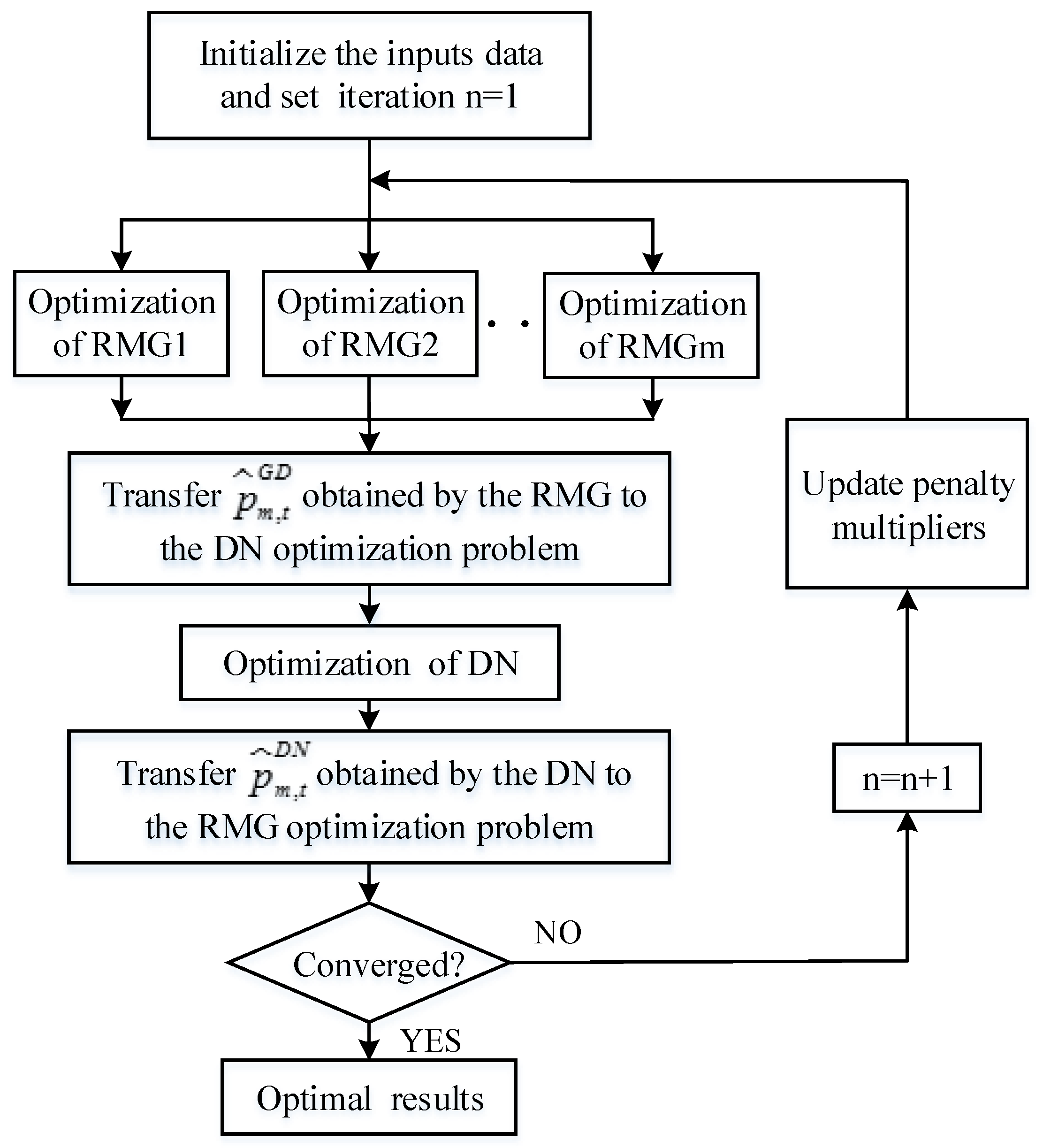
4. The Realization of ATC-Based Distributed Coordinated Optimization

As mentioned in Section 3.1, a proper penalty function $\pi (·)$ is required to relax the consistency constraints in the local objective functions of RMGs and ADN, and then an iterative procedure can be executed to enforce the difference between virtual generator and virtual load to be small enough and find the optimal coordinated operation point of the entities. Augmented Lagrangian relaxation with an alternating direction method of multipliers is adopted to model the penalty function $\pi (·)$ [32], and it has a good convergence property for the convex optimization problem [28]. Thus, the optimization objectives of RMGs and ADN can be rewritten respectively as follows:

$$\min F_{RMGm}+{\displaystyle \sum _{t=1}^T[{\alpha }_{m,t}(p_{m,t}^{\mathrm{GD}}-{\widehat{p}}_{m,t}^{DN})}+{\beta }_{m,t}{\Vert p_{m,t}^{\mathrm{GD}}-{\widehat{p}}_{m,t}^{DN}\Vert }_2^2]$$

(30)

$$\min F_{ADN}+{\displaystyle \sum _{t=1}^T}{\displaystyle \sum _{m=1}^{N_{RMG}}[{\alpha }_{m,t}(p_{m,t}^{\mathrm{DN}}-{\widehat{p}}_{m,t}^{GD})+{\beta }_{m,t}{\Vert p_{m,t}^{\mathrm{DN}}-{\widehat{p}}_{m,t}^{GD}\Vert }_2^2]}$$

(31)

The flowchart of ATC-based distributed optimal coordinated operation of ADN with multi-RMGs is shown in Figure 5. The corresponding steps are illustrated as follows:

Step 1. Initialize the input data. Set the initial values of the coupling variables ($p_m^{\mathrm{DN}}$, $p_m^{\mathrm{GD}}$) and the Augmented Lagrangian penalty multipliers ${\alpha }_m$, ${\beta }_m$ and $\gamma$, set the ATC convergence tolerances, set iteration index to n = 1.

Step 2. Each RMG solves its own optimization problem independently and transfers its optimal virtual generation ${\widehat{p}}_m^{\mathrm{GD}}$ to the ADN level. In this step, the optimization problems in RMG level are optimized in parallel.

Step 3. After receiving ${\widehat{p}}_m^{\mathrm{GD}}$ from the RMGs, the ADN solves its optimization problem of (29). Then its optimal virtual load ${\widehat{p}}_m^{DN}$ is obtained and transmitted to the connected RMGs.

Step 4. Check the following termination criteria (32) and (33).

$$G_{ap}={\Vert p_{m,t}^{\mathrm{GD},\mathrm{n}}-p_{m,t}^{DN,n}\Vert }_{\infty }\le {\delta }_1$$

(32)

$$R_{el}=\left|\frac{(F_{ADN}^n-F_{ADN}^{n-1})+{\displaystyle \sum _{m=1}^{N_{RMG}}(F_{RMGm}^n-F_{RMGm}^{n-1})}}{F_{ADN}^n+{\displaystyle \sum _{m=1}^{N_{RMG}}{F}_{RMGm}^n}}\right|\le {\delta }_2$$

(33)

In the above formulation, the subscript n or (n-1) represents the nth or (n-1)th iteration. $G_{ap}$ denotes the mismatch between the virtual generation and virtual load, which reflects the maximum gap in consistency constraints. $R_{el}$ denotes the relative difference in objective function between two consecutive loop iterations. ${\delta }_1$ and ${\delta }_2$ represent pre-determined convergence tolerances. If the inequalities (32) and (33) both are satisfied, the iterative process stops, and the converged optimal result is obtained, otherwise, go to Step 5.

Step 5. Set n=n+1 and update the Augmented Lagrangian penalty multipliers according to (34), and then return to Step 2.

$$\begin{array}{l}{\alpha }_{m,t}^n={\alpha }_{m,t}^{n-1}+2{({\beta }_{m,t}^{n-1})}^2(p_{m,t}^{\mathrm{GD},\mathrm{n}-1}-p_{m,t}^{DN,n-1})\hspace{1em}\hspace{1em}\alpha ,\beta \in (0,2)\\ {\beta }_{m,t}^n=\gamma {\beta }_{m,t}^{n-1}\hspace{1em}\hspace{1em}1\le \gamma \le 3\end{array}$$

(34)

5. The Realization of ATC-Based Distributed Coordinated Optimization

5.1. Test System and Data

The case study is conducted on the modified IEEE-33 bus distribution system to coordinate the energy management and optimal operation between RMGs and ADN during 24 h of operation as shown in Figure 6.

The RMGs are connected to bus 1–18 in the IEEE 33-bus system. Every RMG includes 50 households andare considered to have the same load-demand profile. The 24-h load-demand profile for a typical household is shown in Figure 7. The daily load curve for the remaining buses of the IEEE 33-bus system and time-of-use (TOU) electricity price are illustrated in Figure 8. Their controllable DGs are connected to buses 22, 23 and 27 respectively, and their corresponding rated active power is 3MW, 3.5MW and 4.5MW. The corresponding parameter settings for the ATC algorithm are: ${\alpha }_m$ = ${\beta }_m$ = 1, $\gamma$ = 2, ${\delta }_1$ = 0.01, ${\delta }_2$ = 0.001. The proposed optimization problems are implemented in MATLAB2015 utilizing the CPLEX12.5 solver [31].

5.2. Simulation Results and Discussion

In the RMGs level, the optimization problems of energy management are solved in parallel. The optimized result of energy resources scheduling for an arbitrarily specified RMG is shown in Figure 9.

It is obvious that flexible and EVs charging loads can effectively aid the peak clipping and valley filling by increasing the use of power energy during off-peak periods while reducing the amount of electric power used during on-peak periods. According to the optimized results, the flexible loads are put into operation between 01:00 hrs and 06:00 hrs, while the EVs are charged between 02:00 hrs and 06:00 hrs and at 12:00 hrs with lower prices. During peak hours (18:00 hrs to 22:00 hrs), EVs provide power supply to the household loads in the RMG by V2H discharging. During daylight hours, the electric power consumed by household loads is covered from the purchased electricity from the DN and PV generation.

The RMG is the aggregate of household prosumers, the optimized scheduling result of EV and flexible loads for a household prosumer within the RMG is shown in Figure 10.

By comparing Figure 10 and Figure 7, it is obvious that the shiftable loads are allocated during the off-peak hours inline with the lower energy prices, and the EV’s battery is also charged when electricity prices are relatively lower (i.e., early morning). Moreover, it can be seen that the EV battery is used as electricity storage for household loads and provides a V2H service during peak load period, i.e., the energy stored in the EV’s battery supplies the domestic loads from 18:00 hrs to 22:00 hrs during the peak load period. Moreover, it can be seen that the household prosumer has two hours of autonomous operation, i.e., during 10:00 hrs and 18:00 hrs when RMG is independent of the main grid. The advantage is assisted by rooftop PV generation, demand responses of EV and flexible loads.

Energy consumption cost minimization is a major objective for every household prosumer.

Table 1. Energy Comparative Costs ($/day) for a Typical Household.

Energy Cost	Un-Optimized Case	Proposed Energy Coordinated Mode
Inflexible loads	7.7	7.7
EV charging + Flexible loads	9.93	3.06
PV Generation	−0.5	−0.5
V2H	0	−5.22
Daily energy cost	17.13	5.02

shows the daily energy costs based on TOU electricity price for a typical household in RMG level under the un-optimized case and the proposed energy coordinated mode. The positive values mean the amount of energy cost that a household prosumer is required to pay, and the negative values mean the amount of the cost saved.

From Table 1 it can be seen that shifting EV charging and flexible loads from high-demand hours to off-peak hours a significant amount of cost can be saved. The cost went down from $9.93 to $3.06, a reduction in the cost about 69%. The V2H system usage also brings a respectable energy cost saving ($5.22) to individual household prosumer.

Figure 11 shows the power scheduling results of controllable DGs in the distribution network from the proposed method in the minimum cost operational solution of ADN.

Blue is the cumulate profile under the un-optimized case while red is the cumulate profile under the proposed distributed optimal coordinated operation mode. It is obvious that the output power of all sources in the distribution system level becomes smooth after optimizing since the proposed method allows for optimized scheduling of demand responses to household prosumers in the RMG level so that shifting electric demand from on-peak periods to off-peak periods. It illustrates that the proposed method includes coordinating RMGs and distribution system operation strategy to have peak shaving and smoothing for distribution load curve at the same time, which can benefit distribution system operators through existing grid capacity upgrade/expansion deferrals.

Table 2. Daily Operating Costs and Active Power Losses for the Distribution Network.

Comparison Item	Un-Optimized Case	Optimal Coordinated Operation Mode
Operation cost ($)	37,597	21,911
Power loss (kW)	5812	4767

illustrates the daily operating costs and the active power losses for the distribution network under the un-optimized case and the proposed optimal coordinated operation mode.

It can be derived from the above results that the operating cost and power loss has been reduced by 41.72% and 17.98% respectively during a day based on the proposed ATC-based distributed optimal coordinated operation method. It shows that the proposed method provides an effective solution for distribution system operators to improve economic operation and energy efficiency of DN.

Figure 12 depicts the evolution of the proposed ATC-based method. According to the pre-determined convergence thresholds the method converges within 19 iterations. When it converged, the total computation time consumed by the proposed method is 91.8s. As shown in Figure 12a, the maximal difference between virtual generation and virtual load $G_{ap}$ is smaller than 0.01, while the relative difference in optimal feasible solutions $R_{el}$ is smaller than 0.001, as shown in Figure 12b.

It should be noted that the proposed hierarchical optimization uses a deterministic load modeling approach, but the iterative process in analytical target cascading algorithm based distributed optimization will convergence regardless of stochasticity [28] in load, although the global optimum, and thus number of iterations and the point of convergence, will be affected.

The solutions to the proposed distributed method and the centralized method are compared in

Table 3. Comparison Results.

Total Objective Function fdis (Proposed Method)	Total Objective Function fcen (Centralized Method)	Relative Error (fdis − fcen)/fcen
$26,519	$26,137	0.0146

, the distributed result is close to the centralized result and relative error is 0.0146. It shows that the proposed ATC-based distributed coordinated method provides a feasible and effective solution to coordinate energy management and optimal operation between the RMGs and ADN.

It should be mentioned that our design in this paper focuses on providing an interrelation between ADN and RMGs and aims at coordinating optimal hourly energy consumption scheduling and operation management between the two entities. Although simplified EV and shiftable load models and constant household profiles are adopted for simplicity in this work, the flexibility and generality of the proposed hierarchical optimization framework makes it suitable for further considering load modeling with better accuracy and rationality.

6. Conclusions and Future Works

In this paper, a hierarchical structure of DN integration of multi-RMGs is presented while considering the household prosumers cluster as an RMG. The RMG integrating into future distribution system has significant potentials to improve energy efficiency and economic benefits for the RMGs and ADN by coordinating optimal energy consumption scheduling and operation management between the two entities. A distributed coordination and hierarchical optimization method based on ATC is proposed for residential microgrids integrated into the distribution system while considering the demand responses of EVs and flexible loads in households and the underlying power flow balance constraints in distribution network level. Based on that, the optimization problems of RMGs and ADN are completely separated from each other and solved independently. A case study is provided to prove the feasibility and effectiveness of the proposed method. The test results show that the method performs an effective function on peak-load shifting and jointly maximizing the welfare of both household prosumers and distribution system operator.

There are several directions that the proposed hierarchical optimization framework can be further extended.

• Energy consumption behaviors of households are considered to be the same in small-scale residential areas and constant household profiles are adopted, which is simplified. The proposed hierarchical optimization framework will be extended to a stochastic bi-level programming problem considering individual household profiles in our future work, which can be tackled by using the scenario-based optimization approach.
• Energy interactions among the individual household prosumers within RMG while taking into account their differences in energy consumption behaviour will be incorporated into the coordinating energy management between the RMGs and ADN.
• There are stochasticity and uncertainty in loads. Popular optimization techniques such as stochastic optimization and robust optimization [33] to deal with load uncertainty in coordinating energy management is an interesting research topic for further works.

References

1. Wu, X.; Hu, X.; Teng, Y.; Qian, S.; Cheng, R. Optimal integration of a hybrid solar-battery power source into smart home nanogrid with plug-in electric vehicle. J. Power Sources 2017, 363, 277–283. [Google Scholar] [CrossRef] [Green Version]
2. Luna, A.C.; Diaz, N.L.; Graells, M.; Vasquez, J.C.; Guerrero, J.M. Cooperative energy management for a cluster of households prosumers. IEEE Trans. Consum. Electron. 2016, 62, 235–242. [Google Scholar] [CrossRef] [Green Version]
3. Ericson, T. Households’ self-selection of dynamic electricity tariffs. Appl. Energy 2011, 88, 2541–2547. [Google Scholar] [CrossRef]
4. Liu, N.; Chen, Q.; Liu, J.; Lu, X.; Li, P.; Lei, J.; Zhang, J. A heuristic operation strategy for commercial building microgrids containing EVs and PV system. IEEE Trans. Ind. Electron. 2015, 62, 2560–2570. [Google Scholar] [CrossRef]
5. Pedrasa, M.A.A.; Spooner, T.D.; MacGill, I.F. Coordinated scheduling of residential distributed energy resources to optimize smart home energy services. IEEE Trans. Smart Grid 2010, 1, 134–143. [Google Scholar] [CrossRef]
6. Igualada, L.; Corchero, C.; Cruz-Zambrano, M.; Heredia, F.J. Optimal energy management for a residential microgrid including a vehicle-to-grid system. IEEE Trans. Smart Grid 2014, 5, 2163–2172. [Google Scholar] [CrossRef]
7. Liu, Y.; Qiu, B.; Fan, X.; Zhu, H.; Han, B. Review of smart home energy management systems. Energy Procedia 2016, 104, 504–508. [Google Scholar] [CrossRef]
8. Zhou, B.; Li, W.; Chan, K.W.; Cao, Y.; Kuang, Y.; Liu, X.; Wang, X. Smart home energy management systems: Concept, configurations, and scheduling strategies. Renew. Sustain. Energy Rev. 2016, 61, 30–40. [Google Scholar] [CrossRef]
9. Peacock, A.D.; Chaney, J.; Goldbach, K.; Walker, G.; Tuohy, P.; Salvador, S.; Todoli, D.; Owens, H. Co-designing the next generation of home energy management systems with lead-users. Appl. Ergon. 2017, 60, 194–206. [Google Scholar] [CrossRef] [Green Version]
10. Jin, X.; Baker, K.; Christensen, D.; Isley, S. Foresee: A user-centric home energy management system for energy efficiency and demand response. Appl. Energy 2017, 205, 1583–1595. [Google Scholar] [CrossRef]
11. Ahmad, A.; Khan, A.; Javaid, N.; Hussain, H.M.; Abdul, W.; Almogren, A.; Alamri, A.; Niaz, I.A. An optimized home energy management system with integrated renewable energy and storage resources. Energy 2017, 10, 549. [Google Scholar] [CrossRef]
12. Shakeri, M.; Shayestegan, M.; Reza, S.M.S.; Yahya, I.; Bais, B.; Akhtaruzzaman, M.; Sopian, K.; Amin, N. Implementation of a novel home energy management system (HEMS) architecture with solar photovoltaic system as supplementary source. Renew. Energy 2018, 125, 108–120. [Google Scholar] [CrossRef]
13. Kriett, P.O.; Salani, M. Optimal control of a residential microgrid. Energy 2012, 42, 321–330. [Google Scholar] [CrossRef]
14. Anvari-Moghaddam, A.; Guerrero, J.M.; Vasquez, J.C.; Monsef, H.; Rahimi-Kian, A. Efficient energy management for a grid-tied residential microgrid. IET Gener. Transm. Distrib. 2017, 11, 2752–2761. [Google Scholar] [CrossRef]
15. Wu, X.; Wang, Z.; Du, J.; Wu, G. Optimal operation of residential microgrids in the harbin area. IEEE Access 2018, 6, 30726–30736. [Google Scholar] [CrossRef]
16. Liu, J.H.; Chu, C.C. Iterative distributed algorithms for real-time available transfer capability assessment of multiarea power systems. IEEE Trans. Smart Grid 2015, 6, 2569–2578. [Google Scholar] [CrossRef]
17. Li, Z.; Wu, W.; Zhang, B.; Wang, B. Decentralized multi-area dynamic economic dispatch using modified generalized benders decomposition. IEEE Trans. Power Syst. 2016, 31, 526–538. [Google Scholar] [CrossRef]
18. Peng, Q.; Low, S.H. Distributed optimal power flow algorithm for radial networks, I: Balanced single phase case. IEEE Trans. Smart Grid 2018, 9, 111–121. [Google Scholar] [CrossRef]
19. Kargarian, A.; Mehrtash, M.; Falahati, B. Decentralized implementation of unit commitment with analytical target cascading: A parallel approach. IEEE Trans. Power Syst. 2018, 33, 3981–3993. [Google Scholar] [CrossRef]
20. Kargarian, A.; Fu, Y.; Wu, H. Chance-constrained system of systems based operation of power systems. IEEE Trans. Power Syst. 2016, 31, 3404–3413. [Google Scholar] [CrossRef]
21. Mohammadi, A.; Mehrtash, M.; Kargarian, A. Diagonal quadratic approximation for decentralized collaborative TSO + DSO optimal power flow. IEEE Trans. Smart Grid 2018, 10, 2358–2370. [Google Scholar] [CrossRef]
22. Kargarian, A.; Mohammadi, J.; Guo, J.; Chakrabarti, S.; Barati, M.; Hug, G.; Kar, S.; Baldick, R. Toward distributed/decentralized DC optimal power flow implementation in future electric power systems. IEEE Trans. Smart Grid 2018, 9, 2574–2594. [Google Scholar] [CrossRef]
23. Li, Y.; Ng, B.L.; Trayer, M.; Liu, L. Automated residential demand response: Algorithmic implications of pricing models. IEEE Trans. Smart Grid 2012, 3, 1712–1721. [Google Scholar] [CrossRef]
24. Safdarian, A.; Fotuhi-Firuzabad, M.; Lehtonen, M. A distributed algorithm for managing residential demand response in smart grids. IEEE Trans. Ind. Inform. 2014, 10, 2385–2393. [Google Scholar] [CrossRef]
25. Juelsgaard, M.; Andersen, P.; Wisniewski, R. Distribution loss reduction by household consumption coordination in smart grids. IEEE Trans. Smart Grid 2014, 5, 2133–2144. [Google Scholar] [CrossRef]
26. Li, J.; Zhang, C.; Xu, Z.; Wang, J.; Zhao, J.; Zhang, Y.-J.A. Distributed transactive energy trading framework in distribution networks. IEEE Trans. Power Syst. 2018, 33, 7215–7227. [Google Scholar] [CrossRef]
27. Kim, H.M.; Rideout, D.G.; Papalambros, P.Y.; Stein, J.L. Analytical target cascading in automotive vehicle design. J. Mech. Des. 2003, 125, 481–489. [Google Scholar] [CrossRef]
28. Michelena, N.; Park, H.; Papalambros, P.Y. Convergence properties of analytical target cascading. AIAA J. 2003, 41, 897–905. [Google Scholar] [CrossRef]
29. Gao, H.; Liu, J.; Wang, L.; Wei, Z. Decentralized energy management for networked microgrids in future distribution systems. IEEE Trans. Power Syst. 2018, 33, 3599–3610. [Google Scholar] [CrossRef]
30. Low, S.H. Convex relaxation of optimal power flow part I: Formulations and equivalence. IEEE Trans. Control Netw. Syst. 2014, 1, 15–27. [Google Scholar] [CrossRef]
31. ILOG CPLEX Homepage. [Online]. 2018. Available online: http://www.ilog.com (accessed on 6 May 2018).
32. Tosserams, S.; Etman, L.F.P.; Papalambros, P.Y.; Rooda, J.E. An augmented Lagrangian relaxation for analytical target cascading using the alternating direction method of multipliers. Struct. Multidiscip. Optim. 2006, 31, 176–189. [Google Scholar] [CrossRef] [Green Version]
33. Chen, Z.; Wu, L.; Fu, Y. Real-time price-based demand response management for residential appliances via stochastic optimization and robust optimization. IEEE Trans. Smart Grid 2012, 3, 1822–1831. [Google Scholar] [CrossRef]
Figure 1. Conceptual schematic outline of the residential microgrid (RMG), where the solid black line with arrows represents power flow.
Applsci 09 02136 g001
Figure 2. The hierarchical structure of active distribution network (ADN) connected with Multi-RMGs, where the solid line with arrows represents the power flow and the dashed line with arrows represents information flow.
Applsci 09 02136 g002
Figure 3. Conceptual schematic outline of the RMG, where the solid black line with an arrow represents power flow.
Applsci 09 02136 g003
Figure 4. Decoupling scheme of ADN and RMGs.
Applsci 09 02136 g004
Figure 5. Flowchart of analytical target cascading (ATC)-based distributed optimal coordinated operation of ADN with multi-RMGs.
Applsci 09 02136 g005
Figure 6. Modified IEEE-33 bus distribution system.
Applsci 09 02136 g006
Figure 7. The 24-h load-demand profile for a household.
Applsci 09 02136 g007
Figure 8. The 24-h power load curve in the distribution network level and time-of-use (TOU) electricity price.
Applsci 09 02136 g008
Figure 9. Daily scheduling optimization results for the RMG connected to bus 9.
Applsci 09 02136 g009
Figure 10. Optimized daily scheduling results for a typical household prosumer within RMG.
Applsci 09 02136 g010
Figure 11. Optimized daily scheduling results for a typical household prosumer within RMG Power scheduling results of distributed generations in the distribution network (a) Power purchased from the upstream grid, which is indicated as HV; (b) Power output of the DG installed in bus 22; (c) Power output of the DG installed in bus 27; (d) Power output of the DG installed in bus 23.
Applsci 09 02136 g011
Figure 12. The convergence of the ATC-based distributed method: (a) Feasibility, (b) Optimality.
Applsci 09 02136 g012