Design of Terminal Sliding Mode Controllers for Disturbed Non-Linear Systems Described by Matrix Differential Equations of the Second and First Orders

Abstract

This paper describes a design scheme for terminal sliding mode controllers of certain types of non-linear dynamical systems. Two classes of such systems are considered: the dynamic behavior of the first class of systems is described by non-linear second-order matrix differential equations, and the other class is described by non-linear first-order matrix differential equations. These two classes of non-linear systems are not completely disjointed, and are, therefore, investigated together; however, they are certainly not equivalent. In both cases, the systems experience unknown disturbances which are considered bounded. Sliding surfaces are defined by equations combining the state of the system and the expected trajectory. The control laws are drawn to force the system trajectory from an initial condition to the defined sliding surface in finite time. After reaching the sliding surface, the system trajectory remains on it. The effectiveness of the approaches proposed is verified by a few computer simulation examples.

1. Introduction

1.1. Motivation

Stabilization of non-linear systems finds applications in many areas of engineering, particularly in the fields of mechanics, robotics, electronics, and so on [1,2]. Non-linear problems arise when analyzing the dynamical behavior of systems, such as robot manipulators with flexible links, different types of oscillators, electrical and electronic circuits, buildings, bridges, and even embedded control systems [3,4,5,6,7]. In some non-linear systems, such as Chua’s circuit, a phenomenon called chaos can be observed [8,9]. This chaotic behavior can be caused, for example, by uncertainties and non-idealities of the electronic circuit elements [10]. The main objective of this paper is to develop a terminal sliding mode stabilization technique for two classes of non-linear systems with dynamic behavior. The first class of systems considered in the paper is described by non-linear matrix differential equations of the second order. The second class of the systems can be mathematically modeled by non-linear matrix differential equations of the first order. These two classes of non-linear systems are not completely disjointed or mutually exclusive; however, they are not equivalent and, therefore, are investigated together; some theorems might be applicable to both classes, while others might fit well into one class only. Additionally, all systems considered in the analysis can be affected by some unknown external disturbances.

1.2. Related Work

Use of a sliding mode control (SMC) is a robust method that can successfully be applied to control both linear and non-linear systems [11,12,13]. As the structure of the control system may vary during the control process, a SMC is useful for its control versatility and consistency across a variety of different applications (see, e.g., [12,14]). The first step in this approach requires a definition of the appropriate sliding surface [15]. Next, a controller must be designed to derive the state of the system from an initial condition to this sliding surface. When the system reaches the sliding surface, it remains in a so-called sliding mode. When the system is in such a mode, the robustness of the closed-loop system against external disturbances, parameter uncertainties, and variations can be assured. A SMC can be designed in two ways: (1) a linear sliding mode control system (LSMC) is used to asymptotically stabilize the closed-loop system, which means that the system will reach an equilibrium in infinite time [11]; or conversely, (2) a terminal sliding mode control system (TSMC), based on non-linear and non-smooth differential equations, enables finite-time convergence to the equilibrium [16,17]. This paper focuses on the second design of the SMC process. Moreover, it is important to note that modern SMCs are implemented as embedded control systems. A SMC is, then, implemented on a custom hardware platform, designed and configured for the specific application. During this phase, special attention also needs to be paid to the implementation aspects, as outlined in [18].

TSMC-based methods for linear and non-linear systems, with and without external disturbances, have been investigated in many papers. The formal description of the systems usually has differing forms, depending on the control approach applied. In most cases, the system is described by a set of first-order differential equations; however, these are often decomposed into several sub-systems. The second-order form is typically used for mechanics, robotics, mechatronics, and other systems that find applications in many areas of engineering. There have also been papers investigating higher-order forms of mathematical models of the systems when designing the TSMC. The general conclusion, after the literature review, is that there are not many papers where the TSMC has been designed for a general class of systems, as the model of the system may influence both the sliding surface and controller design.

A TSMC for linear second-order systems, with multiple inputs and multiple outputs, was considered in [17]. A similar case, with external disturbances included, was investigated in [19]. In this paper, the mathematical model of the system was decomposed into two sub-systems, where each of them were described by a set of first-order differential equations. Another TSMC, for an uncertain linear multi-variable system analyzed completely in a first-order form, was presented in [20]. A TSMC control for a single-input non-linear control system without disturbances was investigated in [21]. The paper [22] investigated applications of TSMC strategies to rigid robotic manipulators, whose dynamics were described by a second-order non-linear matrix differential equation. Other TSMC strategies, for similar types of systems, have been investigated in [23,24,25,26]. Another TSMC approach was presented in [27,28] for non-linear dynamical systems, including some external disturbances. In [29], a TSMC-based approach was proposed that could eliminate so-called singular phenomena. More enhancements in this research area on the topic of TSMC can be found in [30,31,32]. The TSMC can also be applied to uncertain linear systems, using some fuzzy logic mechanisms, as presented in [33]. In this paper, the system model is decomposed into two first-order sub-systems. A Fuzzy TSMC, for some class of non-linear systems, was developed in [34]; this approach also considered external disturbances which might influence the dynamics of the system. The class of systems in [34] was very similar to the matrix first-order form considered in this paper. With fractional-order calculus attracting recent interest in the control system community [35], the work of [36] also merits mention, where a novel fractional-order non-singular TSMC method was proposed. This new approach has been verified experimentally on a rigid hydraulic manipulator under heavy uncertainties and non-linearities. There are also papers in the literature [37,38] which investigated applications of TSMC techniques to time-delay systems, described mathematically by first-order differential equations. The paper [39] addressed a TSMC for non-linear discrete systems. The system model was given in canonical form, and the non-linearities and disturbances appeared in the last equation. TSMC techniques can also be applied to the system models described by high-order differential equations, as shown in [40].

This paper is based on the results presented in [41], for the class of non-linear systems described by second-order matrix differential equations with external disturbances. The effectiveness of this approach has been illustrated by comparison of the proposed control scheme and other controllers. In particular, the continuous TSMC developed in [25], the non-singular TSMC presented in [23], and the linear dynamic feedback control given in [1] have been compared. The comparison analysis, even if done only for second-order systems, can be representative of other forms of system descriptions. In many cases, even if a particular method deals with a second-order model of the system, further analysis is conducted for a first-order form. As shown in the sections below, a TSMC for a first-order matrix system can somehow be considered as a special and simplified form, due to the lower order of the system, of a TSMC for a second-order matrix system. More recently, in [42], it has been shown and formally proven that two different classes of non-linear control systems can be asymptotically stabilized with the help of the same linear dynamic feedback control law. The dynamic behavior of one class is described by non-linear first-order differential equations, while the other class is modeled by non-linear second-order differential equations.

1.3. Contribution

The main contribution of the paper is a design of the terminal sliding mode control laws for two classes of non-linear dynamical systems. The classes studied in the paper are described by second- and first-order matrix-vector non-linear differential equations. Both classes of systems include external disturbances, which are unknown but bounded. One part of this paper is devoted to explaining the terminal sliding mode control strategy, applied to the class of the non-linear second-order systems, which has already been described in [41]. Based on these results, an extension of the TSCM approach is proposed to another class of non-linear systems, described by first-order differential equations. The first-order form of the mathematical model is the default representation of the system dynamics, and hence, the control laws formulated using this form can be more beneficial from both a theoretical and an applied point of view, even though, in some cases, having the system in the second-order form is more natural for some types of systems. An extension of the results obtained in [41] can be considered to be a more detailed contribution to this paper. It is also shown that these two classes of systems are not equivalent, and that there is no bi-directional transformation from one class to the other. Moreover, putting together the control schemes for the two classes of systems can help to understand the approach taken to prove the theorems, and can probably help in extending it to other classes (e.g., higher orders) of the systems by analogy.

Another type of contribution relates to the design of the sliding surface. In general, there is no standardized method for the selection of sliding surfaces; however, several points are necessary during the design process. Firstly, the sliding mode dynamics produced by the controller must be stable, as control laws designed on the basis of unstable sliding surfaces will not be able to steer the system to the point of equilibrium. In this paper, the selection of a proper sliding surface was influenced by the Lyapunov stability theory. The sliding variable was taken as a function of the tracking error. The sliding surfaces shall also be designed in such a way so as not to exceed the order of the system. Finally, the form of the sliding surface shall assure that the system will reach a stability condition in finite time. The sliding surface proposed for the matrix first-order system was taken as a function of the tracking error and compared to the sliding surface designed for the matrix second-order system, which does not contain a non-linear term. This cannot be considered as a direct simplification of the results presented in [41]. Having the sliding surface in such a simple form, we can conclude that the closed loop reaching the sliding surface in finite time is equivalent to the system reaching the desired trajectory in finite time (a classical stabilization problem).

1.4. Organization of the Paper

The paper is organized as follows. In Section 2, two classes of non-linear systems are mathematically described. In the following section, the main results are given; that is, a design procedure of the terminal sliding mode controllers and proofs that the trajectories of the closed-loop systems can reach the sliding surfaces in finite time and then remain on these surfaces. In Section 4, the concept is applied to exemplary electrical circuit structures, in order to verify the approach presented in the paper, with the help of computer simulation experiments. The conclusions are in outlined in Section 5.

2. Systems Description

2.1. Matrix Second-Order System

Consider a non-linear system, whose dynamics are given by

$$\ddot{\mathit{x}}\left(t\right)+\mathit{F}(\dot{\mathit{x}},\mathit{x})\dot{\mathit{x}}\left(t\right)+\mathit{G}\left(\mathit{x}\right)=\mathit{H}\left(\mathit{x}\right)\mathit{u}\left(t\right)+\mathit{z}(\ddot{\mathit{x}},\dot{\mathit{x}},\mathit{x},t),$$

(1)

where $\mathit{x}\left(t\right)\in \mathbb{X}\subset {\mathbb{R}}^n$ represents the internal state of the system, $\mathit{u}\left(t\right)\in \mathbb{U}\subset {\mathbb{R}}^r$ is the input state, $\mathit{z}(\ddot{\mathit{x}},\dot{\mathit{x}},\mathit{x},t)\in {\mathbb{R}}^n$ is a noise disturbance, $t>0$ is the time, $\mathit{F}:{\mathbb{R}}^n\times {\mathbb{R}}^n\supset \Omega \times \Omega \to {\mathbb{R}}^{n\times n}$, $\mathit{G}:{\mathbb{R}}^n\supset \Omega \to {\mathbb{R}}^n$, $\mathit{H}:{\mathbb{R}}^n\supset \Omega \to {\mathbb{R}}^{n\times r}$, $\Omega \subset {\mathbb{R}}^n$ is a neighborhood of zero ($\mathbf{0}\in {\mathbb{R}}^n$), $\mathbb{X}$ is the internal state space, $\mathbb{U}$ is the input state space, ${\mathbb{R}}^n$ and ${\mathbb{R}}^r$ are vector spaces of column vectors with real elements, and ${\mathbb{R}}^{n\times n}$ (${\mathbb{R}}^{n\times r}$) stands for a matrix with n rows and n columns (n rows and r columns), $n\in \mathbb{N}$, $r\in \mathbb{N}$. The functions $\mathit{F}$, $\mathit{G}$, and $\mathit{H}$ have the following form:

$$\mathit{F}(\mathit{\xi },\mathit{\eta })=\left[\begin{array}{cccc}{f}_{11}(\mathit{\xi },\mathit{\eta })& f_{12}(\mathit{\xi },\mathit{\eta })& \dots & f_{1n}(\mathit{\xi },\mathit{\eta })\\ f_{21}(\mathit{\xi },\mathit{\eta })& f_{22}(\mathit{\xi },\mathit{\eta })& \dots & f_{2n}(\mathit{\xi },\mathit{\eta })\\ ⋮& ⋮& \ddots & ⋮\\ f_{n1}(\mathit{\xi },\mathit{\eta })& f_{n2}(\mathit{\xi },\mathit{\eta })& \dots & f_{nn}(\mathit{\xi },\mathit{\eta })\end{array}\right],$$

(2)

$$\mathit{G}\left(\mathit{\xi }\right)={\left[\begin{array}{cccc}{g}_1\left(\mathit{\xi }\right)& g_2\left(\mathit{\xi }\right)& \dots & g_n\left(\mathit{\xi }\right)\end{array}\right]}^{\mathrm{T}},$$

(3)

$$\mathit{H}\left(\mathit{\xi }\right)=\left[\begin{array}{cccc}{h}_{11}\left(\mathit{\xi }\right)& h_{12}\left(\mathit{\xi }\right)& \dots & h_{1r}\left(\mathit{\xi }\right)\\ h_{21}\left(\mathit{\xi }\right)& h_{22}\left(\mathit{\xi }\right)& \dots & h_{2r}\left(\mathit{\xi }\right)\\ ⋮& ⋮& \ddots & ⋮\\ h_{n1}\left(\mathit{\xi }\right)& h_{n2}\left(\mathit{\xi }\right)& \dots & h_{nr}\left(\mathit{\xi }\right)\end{array}\right].$$

(4)

The system starts from an initial condition, denoted as

$$\dot{\mathit{x}}\left(0\right)={\mathit{x}}_{01}\in {\mathbb{R}}^n,\mathit{x}\left(0\right)={\mathit{x}}_{02}\in {\mathbb{R}}^n.$$

(5)

Assumption 1.

The functions $f_{ij}(·,·)$, $g_i(·)$, and $h_{ik}(·)$, $i,j=1,2,\dots ,n$, $k=1,2,\dots ,r$ and their derivatives, with respect to each variable in the set Ω, are considered to be continuous.

Assumption 2.

The function $\mathit{z}(\ddot{\mathit{x}},\dot{\mathit{x}},\mathit{x},t)$ represents an external noise disturbance, which is unknown but fulfils the following condition:

$${\mathit{z}}^{\max }=\underset{\ddot{\mathit{x}},\dot{\mathit{x}},\mathit{x},t}{max}\mathit{z}(\ddot{\mathit{x}},\dot{\mathit{x}},\mathit{x},t)\ge 0.$$

(6)

Assumption 3.

The matrix $\mathit{H}\left(\mathit{x}\right)$ is non-singular for every $\mathit{x}\in \Omega$.

2.2. Matrix First-Order System

Consider a special case of the system (1) and (5), given as follows:

$$\dot{\mathit{x}}\left(t\right)+\mathit{G}\left(\mathit{x}\right)=\mathit{H}\left(\mathit{x}\right)\mathit{u}\left(t\right)+\mathit{z}(\dot{\mathit{x}},\mathit{x},t),\mathit{x}\left(0\right)={\mathit{x}}_0\in {\mathbb{R}}^n.$$

(7)

The meaning of the system parameters are exactly the same as described in the previous section. It is assumed that Assumptions 1–3 hold for the system (7) as well. The system model being in the form of (7) will allow, as illustrated in following sections, for creation of the terminal sliding model controller in a much more simplified form than in the case of the system (1) and (5). This class of the systems can also be considered as an approximation of the class described in the previous section. This might occur for slowly-varying systems, where the second derivative can be neglected (compared to the first derivative).

3. Controller Design

3.1. TSMC for Matrix Second-Order System

As a first step, define a sliding surface for the system (1) as

$$\mathit{s}\left(t\right)=\mathbf{\Lambda }\mathit{e}\left(t\right)-\mathit{Q}\mathit{\psi }\left({\mathit{e}}_{\mathrm{x}}\right),$$

(8)

where $\mathbf{\Lambda }=\left[\mathit{P}{\mathit{I}}_n\right]$, $\mathit{P}\in {\mathbb{R}}^{n\times n}$ represents a gain matrix, ${\mathit{I}}_n$ is an identity matrix of size n, $\mathit{Q}\in {\mathbb{R}}^{n\times n}$, $\mathit{Q}={\mathit{Q}}^{\mathrm{T}}>0$ is a positive-definite matrix, $\mathit{\psi }:{\mathbb{R}}^n\to {\mathbb{R}}^n$ is an $n\times n$ matrix with entries that are non-linear, non-negative functions of ${\mathit{e}}_{\mathrm{x}}$, and $\mathit{e}\left(t\right)={\left[{\mathit{e}}_{\mathrm{x}}\left(t\right){\mathit{e}}_{\mathrm{dx}}\left(t\right)\right]}^{\mathrm{T}}$ is a vector composed of the actual and expected trajectory ${\mathit{x}}_{\mathrm{d}}\left(t\right)$ and ${\dot{\mathit{x}}}_{\mathrm{d}}\left(t\right)$; that is

$${\mathit{e}}_{\mathrm{x}}\left(t\right)=\mathit{x}\left(t\right)-{\mathit{x}}_{\mathrm{d}}\left(t\right),$$

(9)

$${\mathit{e}}_{\mathrm{dx}}\left(t\right)=\dot{\mathit{x}}\left(t\right)-{\dot{\mathit{x}}}_{\mathrm{d}}\left(t\right).$$

(10)

As a next step, a control law shall be designed to guarantee the existence of the sliding mode in the closed-loop system. Consider the following formula:

$$\begin{array}{cc}\hfill \mathit{u}\left(t\right)=& -\mathit{H}{\left(\mathit{x}\right)}^{-1}\mathbf{\Lambda }\mathit{W}(\dot{\mathit{x}},\mathit{x})+\mathit{H}{\left(\mathit{x}\right)}^{-1}\mathit{Q}\frac{\mathrm{d}\mathit{\psi }\left({\mathit{e}}_{\mathrm{x}}\right)}{\mathrm{d}t}\hfill \\ & +\mathit{H}{\left(\mathit{x}\right)}^{-1}\mathit{P}\left({\dot{\mathit{x}}}_{\mathrm{d}}\left(t\right)+{\ddot{\mathit{x}}}_{\mathrm{d}}\left(t\right)\right)\hfill \\ & -\mathit{H}{\left(\mathit{x}\right)}^{-1}\mathit{S}\left(t\right){\mathit{z}}^{\max }-\sigma \mathit{H}{\left(\mathit{x}\right)}^{-1}\mathit{S}\left(t\right){\mathit{s}}_{\eta }\left(t\right)\hfill \\ & -\gamma \mathit{H}{\left(\mathit{x}\right)}^{-1}\mathit{s}\left(t\right),\hfill \end{array}$$

(11)

where $\sigma >0$ and $\gamma >0$ are positive coefficients,

$$\mathit{W}(\dot{\mathit{x}},\mathit{x})=\left[\begin{array}{c}\dot{\mathit{x}}\\ -\mathit{G}\left(\mathit{x}\right)-\mathit{F}(\dot{\mathit{x}},\mathit{x})\dot{\mathit{x}}\end{array}\right],$$

(12)

$$\mathit{S}\left(t\right)=\mathrm{diag}(\mathrm{sgn}\left(s_1\left(t\right)\right),\mathrm{sgn}\left(s_2\left(t\right)\right),\dots ,\mathrm{sgn}\left(s_n\left(t\right)\right)),$$

(13)

$${\mathit{s}}_{\eta }\left(t\right)={\left[\begin{array}{cccc}|s_1{\left(t\right)|}^{\eta }& |s_2{\left(t\right)|}^{\eta }& \dots & |s_n{\left(t\right)|}^{\eta }\end{array}\right]}^{\mathrm{T}},$$

(14)

and $\eta$ is a ratio of two odd positive integers, such that $0<\eta <1$.

The control input (11) to achieve the required sliding surface dynamics can be considered as a function of several parameters; that is, the matrices $\mathit{P}$, $\mathit{Q}$, and $\mathit{\psi }$ and the scalars $\gamma$, $\sigma$, and $\eta$. Some of these parameters influence the sliding surface (8) itself, as well. We can then define a performance index (objective function) for the closed-loop system for evaluation and comparison purposes. The evaluation and comparison criteria can, for example, include indicators related to tracking accuracy, tracking response, robust performance, control effort, chattering behavior, and so on. Weighting factors can be applied to these indicators to define the level of their importance in the performance index. Considering the criteria that are important from an application-specific point of view and combining them into an objective function gives us an optimization problem, the solution of which leads to the best parameters. The problem of selecting the best values of the parameters, in the sense of the defined objective function, has already shown up in the optimal control design literature [43,44,45].

Theorem 1.

Under the Assumptions 1–3, the trajectory of the system (1), (5), when forced by the control (11), will reach the sliding surface (8), starting from the initial condition (5), within a finite time and then remain on this surface.

Proof. 

Consider the following Lyapunov function,

$$V\left(t\right)=0.5\mathit{s}{\left(t\right)}^{\mathrm{T}}\mathit{s}\left(t\right).$$

(15)

Next, calculate the time derivative of V along the solutions of the system (1),

$$\begin{array}{cc}\hfill \dot{V}\left(t\right)& =\mathit{s}{\left(t\right)}^{\mathrm{T}}\dot{\mathit{s}}\left(t\right)\hfill \\ & =\mathit{s}{\left(t\right)}^{\mathrm{T}}\left(\mathbf{\Lambda }\dot{\mathit{e}}\left(t\right)-\mathit{Q}\frac{\mathrm{d}\mathit{\psi }\left({\mathit{e}}_{\mathrm{x}}\right)}{\mathrm{d}t}\right)\hfill \\ & =\mathit{s}{\left(t\right)}^{\mathrm{T}}\left(\mathit{P}\dot{\mathit{x}}\left(t\right)-\mathit{P}{\dot{\mathit{x}}}_{\mathrm{d}}\left(t\right)+\ddot{\mathit{x}}\left(t\right)-{\ddot{\mathit{x}}}_{\mathrm{d}}\left(t\right)\right)\hfill \\ & -\mathit{s}{\left(t\right)}^{\mathrm{T}}\mathit{Q}\frac{\mathrm{d}\mathit{\psi }\left({\mathit{e}}_{\mathrm{x}}\right)}{\mathrm{d}t}\hfill \\ & =\mathit{s}{\left(t\right)}^{\mathrm{T}}\left(\mathit{P}\dot{\mathit{x}}\left(t\right)-\mathit{P}{\dot{\mathit{x}}}_{\mathrm{d}}\left(t\right)\right)\hfill \\ & -\mathit{s}{\left(t\right)}^{\mathrm{T}}\left(\mathit{F}(\dot{\mathit{x}},\mathit{x})\dot{\mathit{x}}\left(t\right)+\mathit{G}\left(\mathit{x}\right)-\mathit{H}\left(\mathit{x}\right)\mathit{u}\left(t\right)\right)\hfill \\ & +\mathit{s}{\left(t\right)}^{\mathrm{T}}\left(\mathit{z}(\ddot{\mathit{x}},\dot{\mathit{x}},\mathit{x},t)-{\ddot{\mathit{x}}}_{\mathrm{d}}\left(t\right)-\mathit{Q}\frac{\mathrm{d}\mathit{\psi }\left({\mathit{e}}_{\mathrm{x}}\right)}{\mathrm{d}t}\right).\hfill \end{array}$$

(16)

The substitution of (11) into (16) yields:

$$\begin{array}{cc}\hfill \dot{V}\left(t\right)& =-\mathit{s}{\left(t\right)}^{\mathrm{T}}\mathit{S}\left(t\right){\mathit{z}}^{\max }-\sigma \mathit{s}{\left(t\right)}^{\mathrm{T}}\mathit{S}\left(t\right){\mathit{s}}_{\eta }\left(t\right)\hfill \\ & -\gamma \mathit{s}{\left(t\right)}^{\mathrm{T}}\mathit{s}\left(t\right)+\mathit{s}{\left(t\right)}^{\mathrm{T}}\mathit{z}(\ddot{\mathit{x}},\dot{\mathit{x}},\mathit{x},t).\hfill \end{array}$$

(17)

Hence, based on Assumption 2,

$$\begin{array}{cc}\hfill \dot{V}\left(t\right)& \le -\gamma {∥\mathit{s}\left(t\right)∥}^2-\sigma {∥\mathit{s}\left(t\right)∥}^{\eta +1}\hfill \\ & =-2\gamma V\left(t\right)-2^{\frac{\eta +1}{2}}\sigma V{\left(t\right)}^{\frac{\eta +1}{2}}.\hfill \end{array}$$

(18)

By taking $\alpha =2\gamma >0$, $\beta =2^{\frac{\eta +1}{2}}\sigma >0$, $\kappa =\frac{\eta +1}{2}$, and according to the thesis of Lemma 1, the trajectory of the system (1) will reach the sliding surface, at least, within a time

$$t_{\mathrm{r}}=\frac{1}{\alpha (1-\kappa )}ln\frac{\alpha V{\left(0\right)}^{1-\kappa }+\beta }{\beta },$$

(19)

where

$$V\left(0\right)=0.5\mathit{s}{\left(0\right)}^{\mathrm{T}}\mathit{s}\left(0\right).$$

(20)

 □

Lemma 1

([19,46]). Consider a continuous positive-definite function $V\left(t\right)$ that satisfies the following inequality

$$\dot{V}\left(t\right)\le -\alpha V\left(t\right)-\beta V{\left(t\right)}^{\kappa },{\forall }_{t\ge t_0},V\left(t_0\right)\ge 0,$$

(21)

where $\alpha >0$, $\beta >0$, and κ is a ratio of two odd positive integers, such that $0<\kappa <1$. Then, for any given time, $t_0$, $V\left(t\right)$ converges to zero, at least, within a finite time, calculated as follows:

$$t_{\mathrm{r}}=t_0+\frac{1}{\alpha (1-\kappa )}ln\frac{\alpha V{\left(t_0\right)}^{1-\kappa }+\beta }{\beta }.$$

(22)

Proof. 

The proof of this lemma can be found in [19]. □

3.2. TSMC for Matrix First-Order System

Define a sliding surface for the system (7) by

$$\mathit{s}\left(t\right)=\mathit{x}\left(t\right)-{\mathit{x}}_{\mathrm{d}}\left(t\right),$$

(23)

where ${\mathit{x}}_{\mathrm{d}}\left(t\right)$ stands for the expected trajectory. In order to enable the sliding mode in the system, design the control law as

$$\begin{array}{cc}\hfill \mathit{u}\left(t\right)=& \mathit{H}{\left(\mathit{x}\right)}^{-1}\left(\mathit{G}\left(\mathit{x}\right)+{\dot{\mathit{x}}}_{\mathrm{d}}\left(t\right)\right)-\mathit{H}{\left(\mathit{x}\right)}^{-1}\mathit{S}\left(t\right){\mathit{z}}^{\max }\hfill \\ & -\sigma \mathit{H}{\left(\mathit{x}\right)}^{-1}\mathit{S}\left(t\right){\mathit{s}}_{\eta }\left(t\right)-\gamma \mathit{H}{\left(\mathit{x}\right)}^{-1}\mathit{s}\left(t\right),\hfill \end{array}$$

(24)

where $\sigma >0$ and $\gamma >0$ are positive coefficients,

$$\mathit{S}\left(t\right)=\mathrm{diag}(\mathrm{sgn}\left(s_1\left(t\right)\right),\mathrm{sgn}\left(s_2\left(t\right)\right),\dots ,\mathrm{sgn}\left(s_n\left(t\right)\right)),$$

(25)

$${\mathit{s}}_{\eta }\left(t\right)={\left[\begin{array}{cccc}|s_1{\left(t\right)|}^{\eta }& |s_2{\left(t\right)|}^{\eta }& \dots & |s_n{\left(t\right)|}^{\eta }\end{array}\right]}^{\mathrm{T}},$$

(26)

where $\eta$ is a ratio of two odd positive integers, such that $0<\eta <1$.

The control input (24) can be considered to be a function of three scalar parameters: $\sigma$, $\gamma$, and $\eta$. The optimal values of these parameters can be identified during the optimization procedure by minimizing a certain objective function, which is defined to achieve particular system performance goals. When the closed-loop system reaches the sliding surface (23), then $\mathit{s}\left(t\right)=\mathbf{0}$, and consequently, $\mathit{x}\left(t\right)={\mathit{x}}_{\mathrm{d}}\left(t\right)$ for $t>t_{\mathrm{r}}$. This means that the trajectory of the system $\mathit{x}\left(t\right)$ reaches the desired trajectory ${\mathit{x}}_{\mathrm{d}}\left(t\right)$. Thus, the formulated problem is equivalent to the classical stabilization problem.

Theorem 2.

Under the Assumptions 1–3, the trajectory of the system (7), when forced by the control (24), will reach the sliding surface (23), starting from the initial condition ${\mathit{x}}_0$, in finite time and then remain on this surface.

Proof. 

Consider the following Lyapunov function candidate for the closed-loop system (7) and (24):

$$V\left(t\right)=0.5\mathit{s}{\left(t\right)}^{\mathrm{T}}\mathit{s}\left(t\right).$$

(27)

Calculating the time derivative of V and presenting it along the solutions of the system (7) gives

$$\begin{array}{cc}\hfill \dot{V}\left(t\right)& =\mathit{s}{\left(t\right)}^{\mathrm{T}}\dot{\mathit{s}}\left(t\right)\hfill \\ & =\mathit{s}{\left(t\right)}^{\mathrm{T}}\left(\dot{\mathit{x}}\left(t\right)-{\dot{\mathit{x}}}_{\mathrm{d}}\left(t\right)\right)\hfill \\ & =\mathit{s}{\left(t\right)}^{\mathrm{T}}\left(-\mathit{G}\left(\mathit{x}\right)+\mathit{H}\left(\mathit{x}\right)\mathit{u}\left(t\right)+\mathit{z}(\dot{\mathit{x}},\mathit{x},t)-{\dot{\mathit{x}}}_{\mathrm{d}}\left(t\right)\right).\hfill \end{array}$$

(28)

Substitution of (24) into (28) yields

$$\dot{V}\left(t\right)=-\mathit{s}{\left(t\right)}^{\mathrm{T}}\mathit{S}\left(t\right){\mathit{z}}^{\max }-\sigma \mathit{s}{\left(t\right)}^{\mathrm{T}}\mathit{S}\left(t\right){\mathit{s}}_{\eta }\left(t\right)-\gamma \mathit{s}{\left(t\right)}^{\mathrm{T}}\mathit{s}\left(t\right)+\mathit{s}{\left(t\right)}^{\mathrm{T}}\mathit{z}(\dot{\mathit{x}},\mathit{x},t).$$

(29)

By Assumption 2, it follows that

$$\dot{V}\left(t\right)\le -\gamma {∥\mathit{s}\left(t\right)∥}^2-\sigma {∥\mathit{s}\left(t\right)∥}^{\eta +1}=-2\gamma V\left(t\right)-2^{\frac{\eta +1}{2}}\sigma V{\left(t\right)}^{\frac{\eta +1}{2}}.$$

(30)

By taking $\alpha =2\gamma >0$, $\beta =2^{\frac{\eta +1}{2}}\sigma >0$, $\kappa =\frac{\eta +1}{2}$, and according to the thesis of Lemma 1, the trajectory of the system (7) will reach the sliding surface in finite time, and after that, remain on this surface. □

4. Illustrative Examples

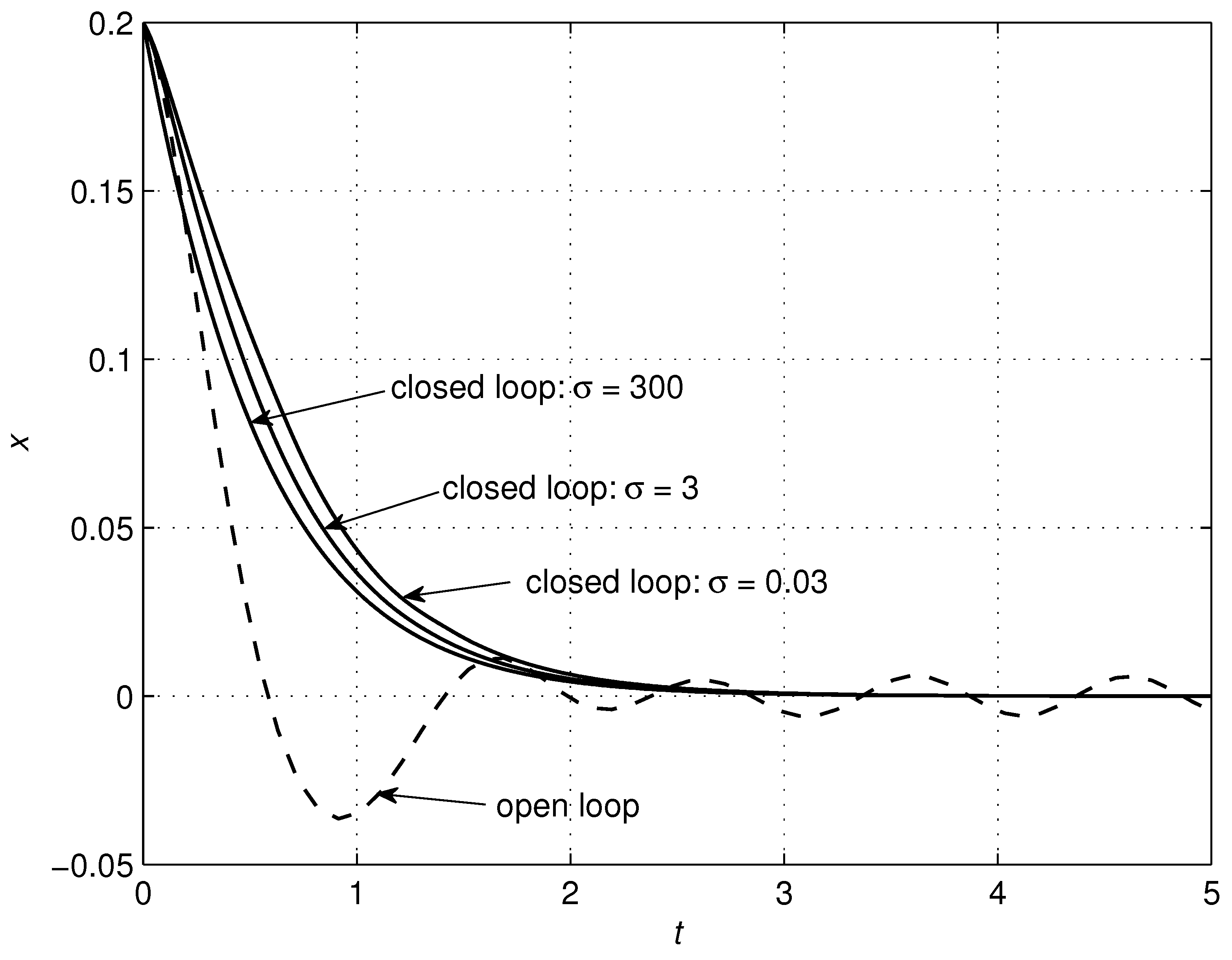
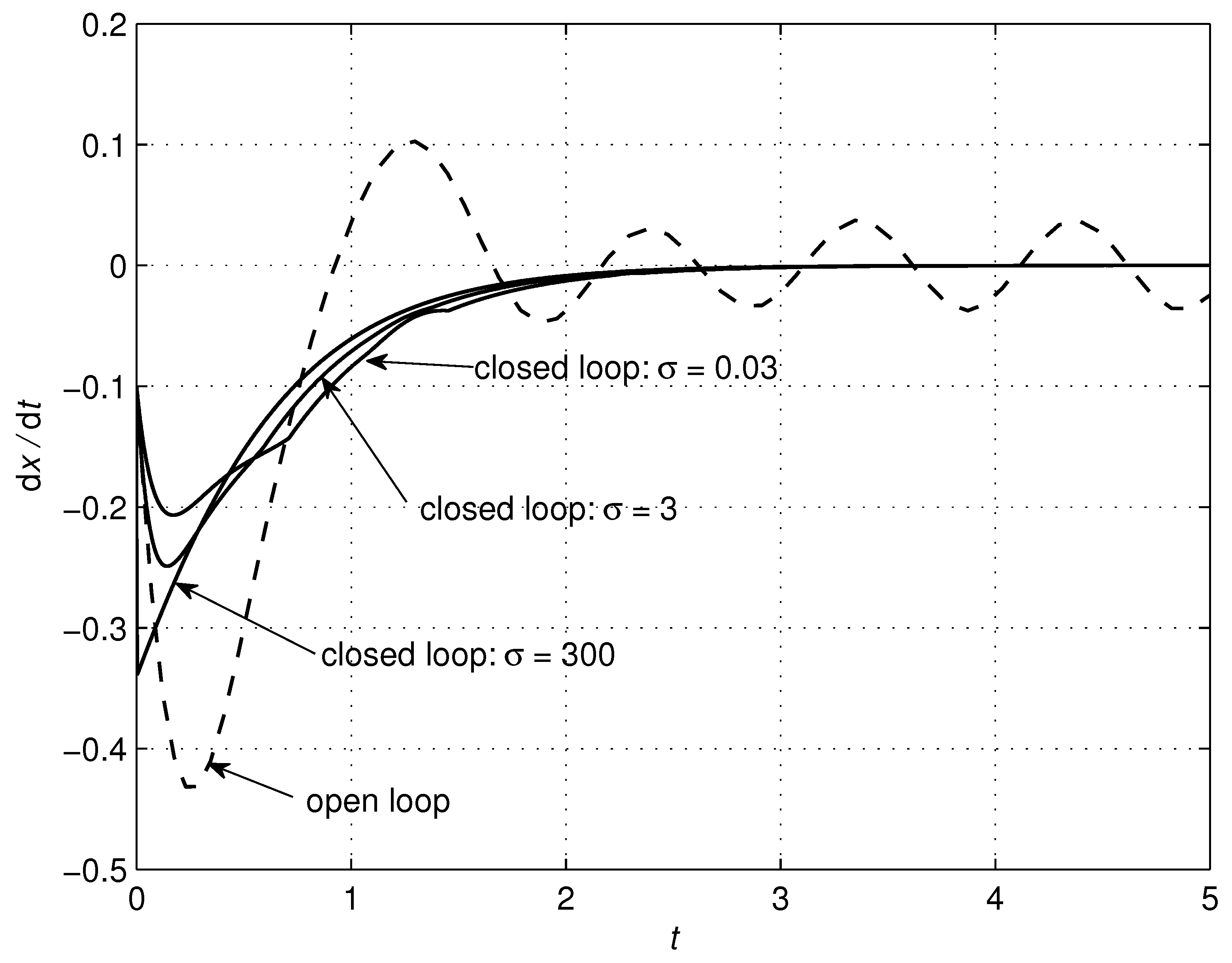
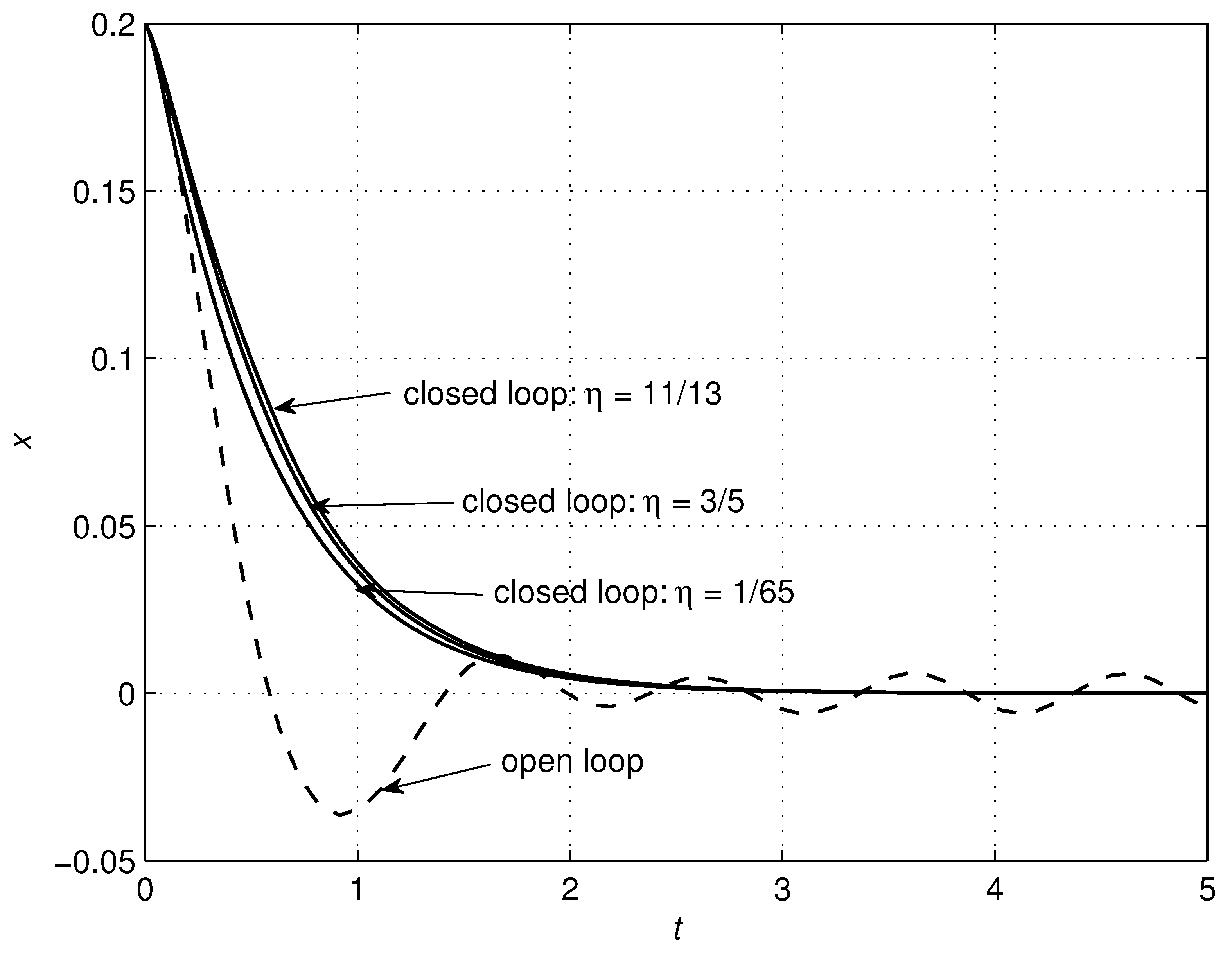
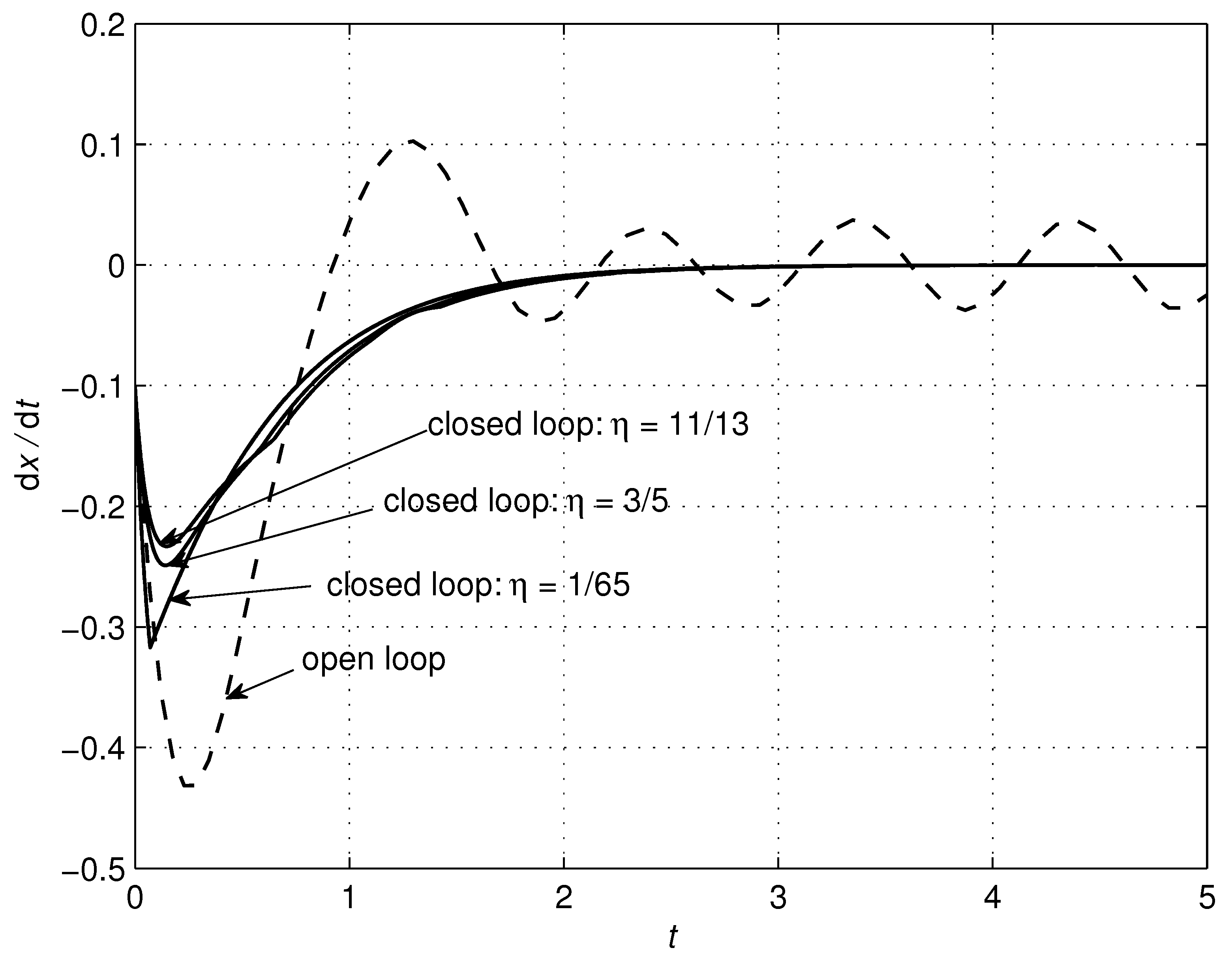
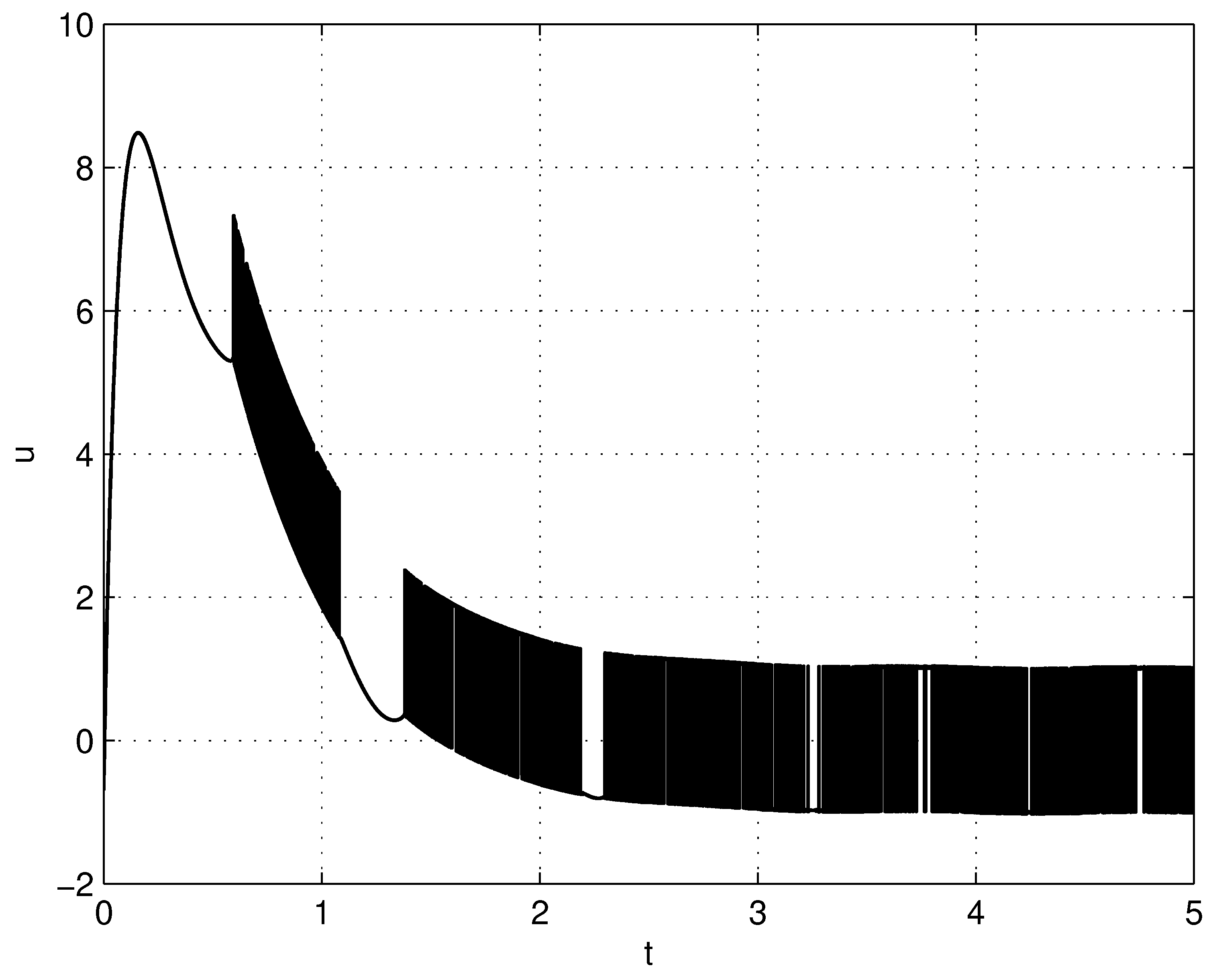
4.1. RLC Circuit

Consider a simple electrical circuit (see Figure 1) which consists of (connected in series) an inductor, a resistor, a capacitor (R-resitor, L-inductor, C-capacitor – RLC), and a voltage source. The resistor and capacitor are considered to be non-linear electrical elements, which means that they have non-linear characteristics. In the circuit presented in Figure 1, there also exists a noise signal, such that

$$z_{\mathrm{u}}^{\max }=\underset{i,t\ge 0}{max}{z}_{\mathrm{u}}(i,t)\ge 0.$$

(31)

The dynamic behaviour of the circuit can be described by the equation:

$$L\frac{\mathrm{d}i\left(t\right)}{\mathrm{d}t}+R\left(i\right)i\left(t\right)+\frac{q\left(t\right)}{C\left(q\right)}=u\left(t\right)+z_{\mathrm{u}}(i,t).$$

(32)

Denote $x\left(t\right)=q\left(t\right)$, $\dot{x}\left(t\right)=\dot{q}\left(t\right)=i\left(t\right)$, $F\left(\dot{x}\right)=L^{-1}R\left(\dot{x}\right)$, $G\left(x\right)=L^{-1}C{\left(x\right)}^{-1}$, $H=L^{-1}$, and $z(\dot{x},t)=L^{-1}{z}_{\mathrm{u}}(\dot{x},t)$. Then, the equation (32) can be presented in the form of (1).

Table 1. List of the RLC (R-resitor, L-inductor, C-capacitor) circuit and terminal sliding mode control system (TSMC) parameters.

RLC Circuit			Controller
Parameter	Value	Unit	Parameter	Value	Unit
$C\left(q\right)$	${10}^{-2}\left(1+0.2{\mathrm{e}}^{-0.1q^2}\right)$	$\mathrm{F}$	$x_{\mathrm{d}}\left(t\right)$	0	$\mathrm{C}$
$i\left(0\right)$	$-0.1$	$\mathrm{A}$	P	2	$\mathrm{A}·{\mathrm{C}}^{-1}$
L	5	$\mathrm{H}$	Q	$1.5$	$\mathrm{A}·{\mathrm{C}}^{-2}$
$R\left(i\right)$	$10\left(1+{\mathrm{e}}^{-0.1i^2}\right)$	$\mathrm{Ohm}$	$\psi \left(e_{\mathrm{x}}\right)$	$e_{\mathrm{x}}^2$	${\mathrm{C}}^2$
$q\left(0\right)$	$0.2$	$\mathrm{C}$	$\gamma$	10	$\frac{\mathrm{V}}{\mathrm{H}·\mathrm{C}}$
$z_{\mathrm{u}}(i,t)$	$sin\left(2\pi t\right)$	$\mathrm{V}$	$\eta$	$3/5$	−
$z^{\max }$	$0.2$	$\mathrm{V}·{\mathrm{H}}^{-1}$	$\sigma$	3	$\frac{\mathrm{V}}{\mathrm{H}·{\mathrm{C}}^{1+\eta }}$

contains a list of the circuit and controller parameters. The values for these parameters have been chosen mostly heuristically, trying to cover the largest possible range of parameter variability. In order to achieve particular system performance objectives, a proper performance index shall be defined, and values of the parameters can then be obtained as a result of solving the optimization problem. This type of optimization problem can be quite easily solved by using numerical optmization methods. It is also easy to check that Assumptions 1–3 are valid. The simulation results are shown in Figure 2, Figure 3, Figure 4, Figure 5, Figure 6, Figure 7 and Figure 8. The results confirm the property of finite-time convergence of the closed-loop system, as well as robustness to disturbances.

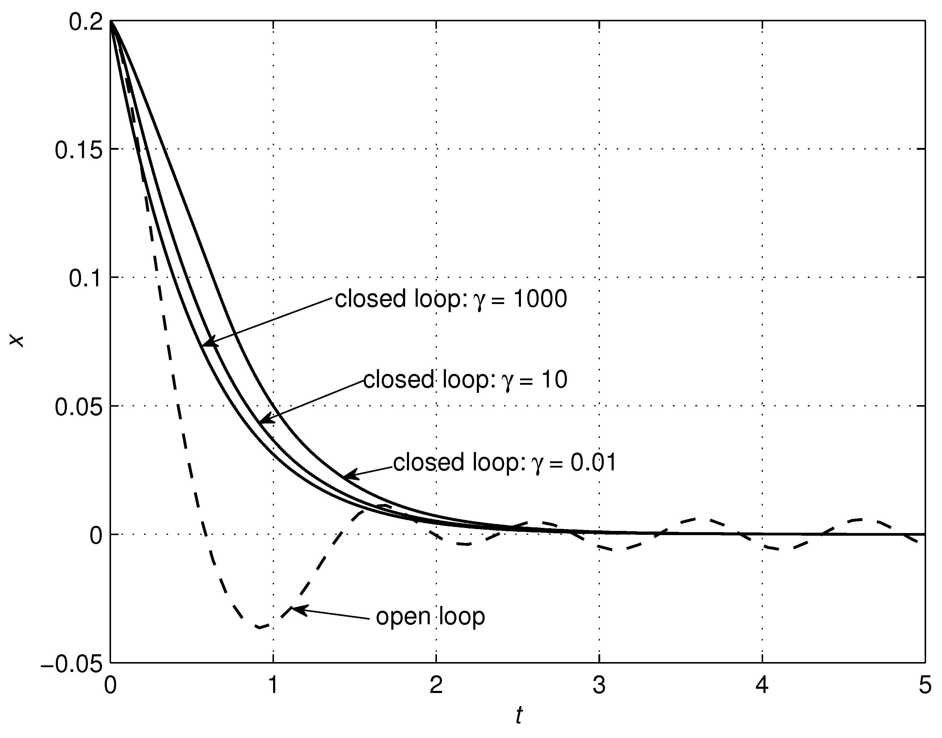
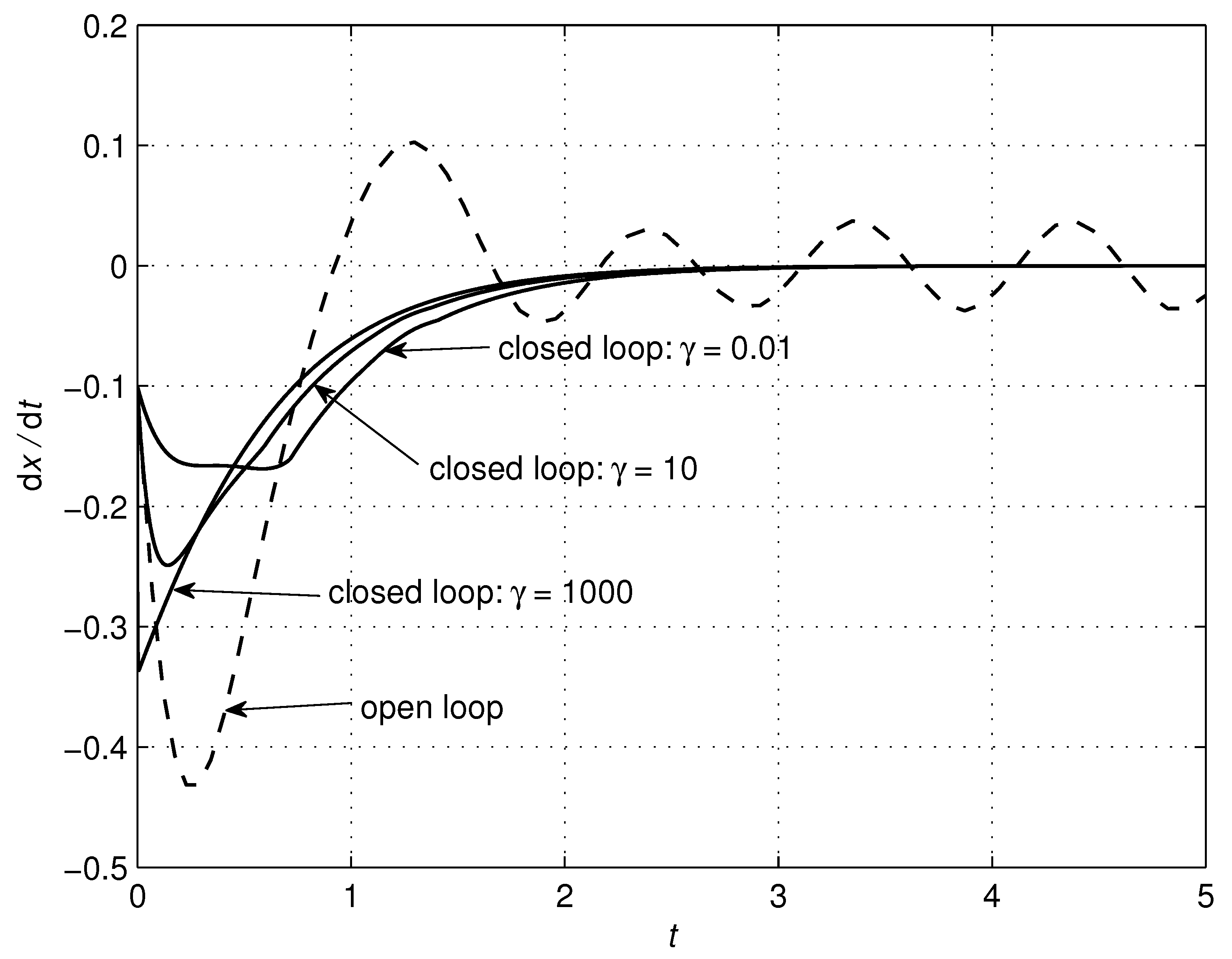
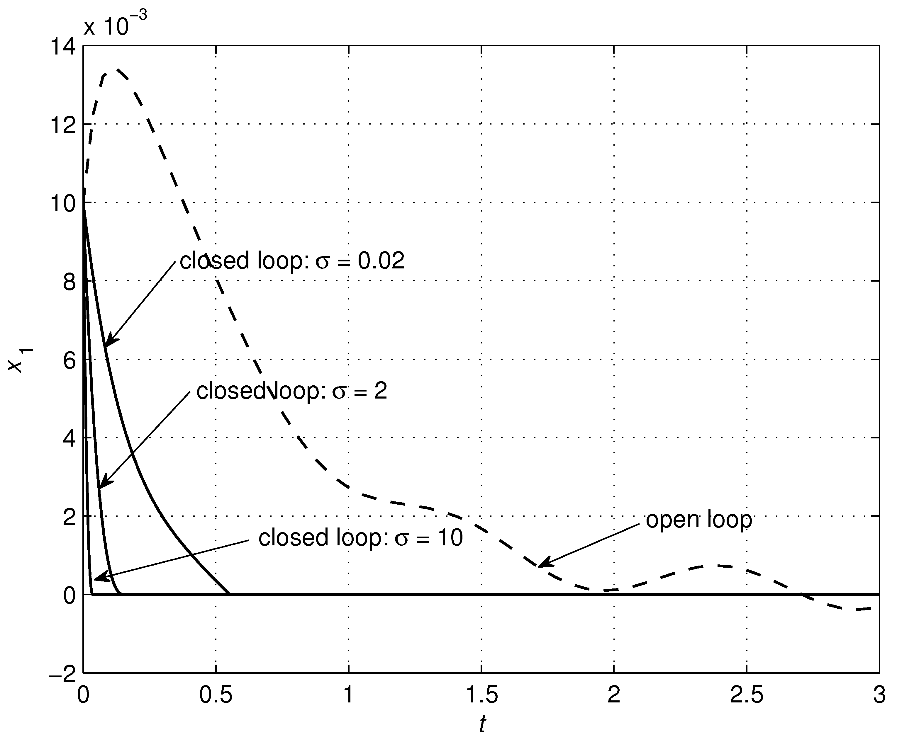
4.2. RC Circuit

Consider, now, another non-linear analog circuit, as shown in Figure 9.

This circuit consists of two power sources, two resistors, and two non-linear capacitors. Additionally, the circuit is disturbed by a noise signal.

The dynamics of electric charge flow in the circuit can be described by the following equations (based on Kirchhoff’s current and voltage laws):

$$R_1{\dot{p}}_1\left(t\right)+\frac{1}{C_1\left(q_1\right)}\left(p_1\left(t\right)-p_2\left(t\right)\right)=u_1\left(t\right)+z_{\mathrm{u}}({\dot{p}}_1,t),$$

(33)

$$R_2{\dot{p}}_2\left(t\right)-\frac{1}{C_1\left(q_1\right)}\left(p_1\left(t\right)-p_2\left(t\right)\right)+\frac{1}{C_2\left(q_2\right)}{p}_2\left(t\right)=u_2\left(t\right),$$

(34)

with given initial conditions $p_1\left(0\right)$ and $p_2\left(0\right)$. The system parameters are shown in

Table 2. Parameters of the RC circuit.

Parameter	Value	Unit
$C_1\left(q_1\right)$	${10}^{-3}\left(1+0.2{\mathrm{e}}^{-0.1q_1^2}\right)$	$\mathrm{F}$
$C_2\left(q_2\right)$	${10}^{-3}\left(2-0.3{\mathrm{e}}^{-0.2q_2^2}\right)$	$\mathrm{F}$
$p_1\left(0\right)$	$0.01$	$\mathrm{C}$
$p_2\left(0\right)$	$0.02$	$\mathrm{C}$
$R_1$	100	$\mathrm{Ohm}$
$R_2$	200	$\mathrm{Ohm}$
$z_{\mathrm{u}}(i_1,t)$	$0.5sin\left(2\pi t\right)$	$\mathrm{V}$
${\mathit{z}}^{\max }$	${\left[0.0050\right]}^{\mathrm{T}}$	${\left[\frac{\mathrm{V}}{\mathrm{Ohm}}\frac{\mathrm{V}}{\mathrm{Ohm}}\right]}^{\mathrm{T}}$

.

Introduce the state variable $\mathit{x}\left(t\right)={\left[x_1\left(t\right)x_2\left(t\right)\right]}^{\mathrm{T}}$, where $x_1\left(t\right)=p_1\left(t\right)$, $x_2\left(t\right)=p_2\left(t\right)$ and the control vector $\mathit{u}\left(t\right)={\left[u_1\left(t\right)u_2\left(t\right)\right]}^{\mathrm{T}}$. Without loss of generality, it can be considered that

$$C_1\left(q_1\right)=C_1(p_1,p_2)=C_1\left(\mathit{x}\right),C_2\left(q_2\right)=C_2\left(p_2\right)=C_2\left(\mathit{x}\right).$$

(35)

Then, the Equations (33) and (34) can be rewritten in the form (7), assuming that

$$\mathit{G}\left(\mathit{x}\right)=\left[\begin{array}{cc}{R}_1^{-1}& 0\\ 0& R_2^{-1}\end{array}\right]\left[\begin{array}{c}{C}_1{\left(\mathit{x}\right)}^{-1}{x}_1-C_1{\left(\mathit{x}\right)}^{-1}{x}_2\\ -C_1{\left(\mathit{x}\right)}^{-1}{x}_1+C_1{\left(\mathit{x}\right)}^{-1}{x}_2+C_2{\left(\mathit{x}\right)}^{-1}{x}_2\end{array}\right],$$

(36)

$$\mathit{H}=\left[\begin{array}{cc}{R}_1^{-1}& 0\\ 0& R_2^{-1}\end{array}\right],$$

(37)

$$\mathit{z}(\dot{\mathit{x}},\mathit{x},t)=\left[\begin{array}{c}{R}_1^{-1}{z}_{\mathrm{u}}(\dot{\mathit{x}},\mathit{x},t)\\ 0\end{array}\right].$$

(38)

It is easy to check that Assumptions 1–3 hold.

The parameters of the controller (24) were chosen according to

Table 3. Parameters of the sliding mode controller.

Parameter	Value	Unit
${\mathit{x}}_{\mathrm{d}}\left(t\right)$	$\mathbf{0}$	${\left[\mathrm{C}\mathrm{C}\right]}^{\mathrm{T}}$
$\gamma$	5	$\frac{\mathrm{V}}{\mathrm{Ohm}·\mathrm{C}}$
$\eta$	$3/5$	−
$\sigma$	2	$\frac{\mathrm{V}}{\mathrm{Ohm}·{\mathrm{C}}^{1+\eta }}$

, with simulation results shown in Figure 10, Figure 11, Figure 12, Figure 13, Figure 14, Figure 15 and Figure 16 to illustrate the effectiveness of the TSMC. The good performance of the system is verified using the proposed control scheme. Both finite-time convergence and robustness to disturbances were guaranteed. Further improvements of the system performance can be achieved through solving an optimization problem where, by minimizing a defined objective function, optimal values of the parameters can be determined.

5. Discussion and Conclusions

It should be noted that the system described by the matrix-vector second-order differential equation (1) is not equivalent to the system described by the matrix-vector differential equation of the first-order (7). Indeed, the system (1) can be rewritten equivalently into the first-order form as:

$$\dot{\tilde{\mathit{x}}}\left(t\right)+\tilde{\mathit{G}}\left(\tilde{\mathit{x}}\right)=\tilde{\mathit{H}}\left(\tilde{\mathit{x}}\right)\mathit{u}\left(t\right)+\tilde{z}(\dot{\tilde{\mathit{x}}},\tilde{\mathit{x}},t),$$

(39)

where

$$\tilde{\mathit{x}}=\left[\begin{array}{c}\mathit{x}\\ \dot{\mathit{x}}\end{array}\right],\tilde{\mathit{z}}=\left[\begin{array}{c}\mathbf{0}\\ \mathit{z}\end{array}\right],\tilde{\mathit{G}}\left(\tilde{\mathit{x}}\right)=\left[\begin{array}{c}\dot{\mathit{x}}\\ \mathit{F}(\dot{\mathit{x}},\mathit{x})\dot{\mathit{x}}+\mathit{G}\left(\mathit{x}\right)\end{array}\right],\mathrm{and}\tilde{\mathit{H}}\left(\tilde{\mathit{x}}\right)=\left[\begin{array}{c}\mathbf{0}\\ \mathit{H}\left(\mathit{x}\right)\end{array}\right].$$

(40)

It is easy to show that the matrix $\tilde{\mathit{H}}$ is non-singular, and that Assumption 3 cannot hold. This means that both systems cannot be considered to be equivalent and should be discussed separately. This is a natural conclusion as, generally, the dynamic properties of second-order differential equations are different to those of first-order differential equations. However, the second class can be considered as an approximation of the first one, which occurs for slowly-varying systems where the second derivative of the system state can be neglected, when compared to the first derivative.

It is well-known that TSMC is very effective in systems subjected to both parameter uncertainties and disturbances. The parameters of the systems considered in this paper had the form of the matrices $\mathit{F}$, $\mathit{G}$, and $\mathit{H}$. The elements of these matrices were, in general, non-linear functions of the system state variables. If the parameter uncertainties can be modeled as continuous functions of the state variables, then it is mathematically proved, by Theorems 1 and 2, that such uncertainties have no influence on the performance of the closed-loop systems, which means that the design control schemes are robust against parameter uncertainties. Such a situation has been demonstrated in the provided examples, where the parameters of the RLC and RC electrical circuits (that is, the capacitances C, $C_1$, $C_2$ and resistance R) contained such types of uncertainties. The case when the parameters of the systems (that is, the elements of the matrices $\mathit{F}$, $\mathit{G}$, and $\mathit{H}$) are also functions of time t has formally neither been covered nor proven. In such a case, we would need to apply an alternative theory more suitable for non-stationary systems. The effectiveness of the proposed control approach has been demonstrated on simple electrical circuits. However, the stabilization scheme can also be applied successfully to mechanical, electromechanical [47], electronic, mechatronic, and even pure software systems.

The most important aspect of this paper is the proof that the trajectory of the closed-loop system reaches, and remains on, the sliding surface after a finite amount of time. This finite time can be calculated analytically. Furthermore, the simulation of the dynamical behavior of electrical circuits with non-linear elements showed the effectiveness of the proposed method. The numerical calculations and computer simulations were performed in the MathWorks™ MATLAB^®/Simulink^® environment (The MathWorks, Inc., Natick, MA, USA). It should be noticed here that in practical applications (and in computer simulations), sliding mode controllers induce high-frequency oscillations, known as chattering in the system output and control. Chattering is a harmful phenomenon, which degrades the performance of the system and can damage its physical components. It can be caused by fast dynamics which were neglected in the model, as well as by digital controllers with a finite sampling rate. There exist various approaches to efficiently reduce the amount of chattering; however, they have not been explored in this paper, as they should be discussed separately.

References

- Skruch, P. Feedback stabilization of a class of nonlinear second-order systems. Nonlinear Dyn. 2010, 59, 681–692. [Google Scholar] [CrossRef]
- Spong, M.; Vidyasagar, M. Robot Dynamics and Control; John Willey & Sons: New York, NY, USA, 2009. [Google Scholar]
- Skruch, P. An educational tool for teaching vehicle electronic system architecture. Int. J. Electr. Eng. Educ. 2011, 48, 174–183. [Google Scholar] [CrossRef]
- Skruch, P.; Panek, M.; Kowalczyk, B. Model-based testing in embedded automotive systems. In Model-Based Testing for Embedded Systems; Zander-Nowicka, J., Schieferdecker, I., Mosterman, P., Eds.; CRC Press: Boca Raton, FL, USA; London, UK; New York, NY, USA, 2011; pp. 293–308. [Google Scholar]
- Długosz, M. Aggregation of state variables in an RC model. Build. Serv. Eng. Res. Technol. 2018, 39, 66–80. [Google Scholar] [CrossRef]
- Długosz, M.; Skruch, P. The application of fractional-order models for thermal process modelling inside buildings. J. Build. Phys. 2016, 39, 440–451. [Google Scholar] [CrossRef]
- Oprzędkiewicz, K.; Gawin, E.; Mitkowski, W. Modeling heat distribution with the use of a non-integer order, state space model. Int. J. Appl. Math. Comput. Sci. 2016, 26, 749–756. [Google Scholar] [CrossRef] [Green Version]
- Moon, F. Chaotic Vibrations: An Introduction for Applied Scientists and Engineers; John Willey & Sons: New York, NY, USA, 2004. [Google Scholar]
- Buscarino, A.; Fortuna, L.; Frasca, M.; Sciuto, G. Chua’s circuit synchronization with diffusive coupling: New results. Int. J. Bifurc. Chaos 2009, 19, 3103–3107. [Google Scholar] [CrossRef]
- Buscarino, A.; Corradino, C.; Fortuna, L.; Frasca, M.; Sprott, J. Nonideal behavior of analog multipliers for chaos generation. IEEE Trans. Circuits Syst. II. Express Briefs 2016, 63, 396–400. [Google Scholar] [CrossRef]
- Edward, C.; Spurgeon, S. Sliding Mode Control: Theory and Appliations; Taylor and Francis: London, UK, 1998. [Google Scholar]
- Liu, J.; Wang, X. Advanced Sliding Mode Control for Mechanical Systems; Springer: Heidelberg, Germany; Dordrecht, The Netherlands; London, UK; New York, NY, USA, 2011. [Google Scholar]
- Pisano, A.; Usai, E. Sliding mode control: A survey with application in math. Math. Comput. Simul. 2011, 81, 954–979. [Google Scholar] [CrossRef]
- Dlugosz, M. Optimization problems of power transmission in automation and robotic. Prz. Elektrotech. 2011, 87, 238–242. [Google Scholar]
- Bandyopadhyay, B.; Deepak, F.; Kim, K. Sliding Mode Control Using Novel Sliding Surfaces; Springer: Berlin/Heidelberg, Germany, 2010. [Google Scholar]
- Liu, J.; Sun, F. A novel dynamic terminal sliding mode control of uncertain nonlinear systems. J. Control Theory Appl. 2007, 5, 189–193. [Google Scholar] [CrossRef]
- Man, Z.; Yu, X. Terminal sliding mode control of MIMO linear systems. IEEE Trans. Circuits Syst. I Fundam. Theory Appl. 1997, 44, 1065–1070. [Google Scholar]
- Skruch, P.; Dlugosz, M.; Mitkowski, W. Mathematical methods for verification of microprocessor-based PID controllers for improving their reliability. Eksploat. I Niezawodn. Maint. Reliab. 2015, 17, 327–333. [Google Scholar] [CrossRef]
- Mobayen, S.; Majd, V.; Sojoodi, M. An LMI-based composite nonlinear feedback terminal sliding-mode controller design for disturbed MIMO systems. Math. Comput. Simul. 2012, 85, 1–10. [Google Scholar] [CrossRef]
- Feng, Y.; Yu, X.; Zheng, J. Nonsingular terminal sliding mode control of uncertain multivariable systems. In Proceedings of the 2006 International Workshop on Variable Structure Systems, Alghero, Italy, 5–7 June 2006; pp. 196–201. [Google Scholar]
- Hong, Y.; Yang, G.; Cheng, D.; Spurgeon, S. A new approach to terminal sliding mode control design. Asian J. Control 2005, 7, 177–181. [Google Scholar] [CrossRef]
- Zhihong, M.; Paplinski, A.; Wu, H. A robust MIMO terminal sliding mode control scheme for rigid robotic manipulators. IEEE Trans. Autom. Control 1994, 39, 2464–2469. [Google Scholar] [CrossRef]
- Feng, Y.; Yu, X.; Man, Z. Non-singular terminal sliding mode control of rigid manipulators. Automatica 2002, 38, 2159–2167. [Google Scholar] [CrossRef]
- Tang, Y. Terminal sliding mode control for rigid robots. Automatica 1998, 34, 51–56. [Google Scholar] [CrossRef]
- Yu, S.; Yu, X.; Shirinzadeh, B.; Man, Z. Continuous finite-time control for robotic manipulators with terminal sliding mode. Automatica 2005, 41, 1957–1964. [Google Scholar] [CrossRef]
- Mezghani, N.; Romdhane, B.; Damak, T. Terminal sliding mode feedback linearization control. Int. J. Sci. Tech. Autom. Control Comput. Eng. 2010, 4, 1174–1187. [Google Scholar]
- Wu, Y.; Yu, X.; Man, Z. Terminal slidingmodecontrol design for uncertain dynamic systems. Syst. Control Lett. 1998, 34, 281–287. [Google Scholar] [CrossRef]
- Xiang, W.; Huangpu, Y. Second-order terminal sliding mode controller for a class of chaotic systems with unmatched uncertainties. Commun. Nonlinear Sci. Numer. Simul. 2010, 15, 3241–3247. [Google Scholar] [CrossRef]
- Li, J.; Yu, F.; Zhang, J.; Feng, J.; Zhao, H. The rapid development of a vehicle electronic control system and its application to an antilock braking system based on hardware-in-the-loop simulation. J. Automob. Eng. 2002, 216, 95–105. [Google Scholar] [CrossRef]
- Chen, F.; Hou, R.; Jiang, B.; Tao, G. Study on fast terminal sliding mode control for a helicopter via quantum information technique and nonlinear fault observer. Int. J. Innov. Comput. Inf. Control 2013, 9, 3437–3447. [Google Scholar]
- Yang, L.; Yang, J. Nonsingular fast terminal sliding-mode control for nonlinear dynamical systems. Int. J. Robust Nonlinear Control 2011, 21, 1865–1879. [Google Scholar] [CrossRef]
- Yu, X.; Zhihong, M. Fast terminal sliding-mode control design for nonlinear dynamical systems. IEEE Trans. Circuits Syst. I Fundam. Theory Appl. 2002, 49, 261–264. [Google Scholar]
- Tao, C.; Taur, J. Adaptive fuzzy terminal sliding mode controller for linear systems with mismatched time-varying uncertainties. IEEE Trans. Syst. Man, Cybern. Part B Cybern. 2004, 34, 255–262. [Google Scholar] [CrossRef]
- Mon, Y. Terminal sliding mode fuzzy-PDC control for nonlinear systems. Int. J. Sci. Technol. Res. 2013, 2, 218–221. [Google Scholar]
- Mitkowski, W.; Skruch, P. Fractional-order models of the supercapacitors in the form of RC lader networks. Bull. Pol. Acad. Sci. Tech. Sci. 2013, 61, 100–106. [Google Scholar]
- Wang, Y.; Luo, G.; Gu, L.; Li, X. Fractional-order nonsingular terminal sliding mode control of hydraulic manipulators using time delay estimation. J. Vib. Control 2016, 22, 3998–4011. [Google Scholar] [CrossRef]
- Feng, Y.; Yu, X.; Zheng, Z. Second-order terminal sliding mode control of input-delay systems. Asian J. Control 2006, 8, 12–20. [Google Scholar] [CrossRef]
- Rasvan, V. Stability and sliding modes for a class of nonlinear time delay systems. Math. Bohem. 2011, 136, 155–164. [Google Scholar]
- Xi, Z.; Hesketh, T. On discrete time terminal sliding mode control for nonlinear systems with uncertainty. In Proceedings of the 2010 Americal Control Conferenece, Baltimore, MD, USA, 30 June–2 July 2010; pp. 980–984. [Google Scholar]
- Zhuang, K.; Su, H.; Zhang, K.; Chu, J. Adaptive terminal sliding mode control for high-order nonlinear dynamic systems. J. Zhejiang Univ.-SCIENCE A 2003, 4, 58–63. [Google Scholar] [CrossRef]
- Skruch, P. A terminal sliding mode control of disturbed nonlinear second-order dynamical systems. J. Comput. Nonlinear Dyn. 2016, 11, 054501. [Google Scholar] [CrossRef]
- Skruch, P.; Dlugosz, M. A linear dynamic feedback controller for non-linear systems described by matrix differential equations of the second and first orders (accepted for publication). Meas. Control 2019, 1–9. [Google Scholar] [CrossRef]
- Alekseev, V.; Tikhomirov, V.; Fomin, S. Optimal Control; Consultants Bureau: New York, NY, USA, 1987. [Google Scholar]
- Boltyanskii, V. Mathematical Methods of Optimal Control; Holt Rinehart & Winston: New York, NY, USA, 1971. [Google Scholar]
- Ioffe, A.; Tikhomirov, V. Theory of Extremal Problems; North-Holland: Amsterdam, The Netherlands, 1979. [Google Scholar]
- Moulay, E.; Peruquetti, W. Finite time stability and stabilization of a class of continuous systems. J. Math. Anal. Appl. 2006, 323, 1430–1443. [Google Scholar] [CrossRef] [Green Version]
- Buscarino, A.; Famoso, C.; Fortuna, L.; Frasca, M. Passive and active vibrations allow self-organization in large-scale electromechanical systems. Int. J. Bifurc. Chaos 2016, 26, 1–10. [Google Scholar] [CrossRef]