We performed simulations with all combinations of cues and communication modes. Each simulation was repeated with 30 random seeds and the data analysis procedure was carried out as discussed in the previous section.
3.1. Presence of Power Law Distributed Features
The analysis of our simulation data shows that in most scenarios there was only weak or no statistical support for the (truncated) power law distribution (see
Figure 2A). In particular, in roughly half of all scenarios no power distributed features were found. This observation suggests that in the present system, scale-free features are rare. Nevertheless, we found 245 + 71 = 316 (truncated) power law distributions with moderate or strong statistical plausibility for different features in various scenario configurations and for both communication modes, DCM and CCM. Thus, our findings are in line with a recent study showing that scale-free networks may occur rarely but across different areas [
55].
As the scatter plots in
Figure 2 show, most of the distributions with weak or moderate support for power law are concentrated below or close to the average values of swarm performance while the distributions with strong support for power law are associated with above-average performance in terms of
and
. Swarm performance was measured using (i) the number of items retrieved by the robots,
, (ii) the average number of collected items per time spent on collision avoidance
, and (iii) the average number of collected items per time spent exploring
.
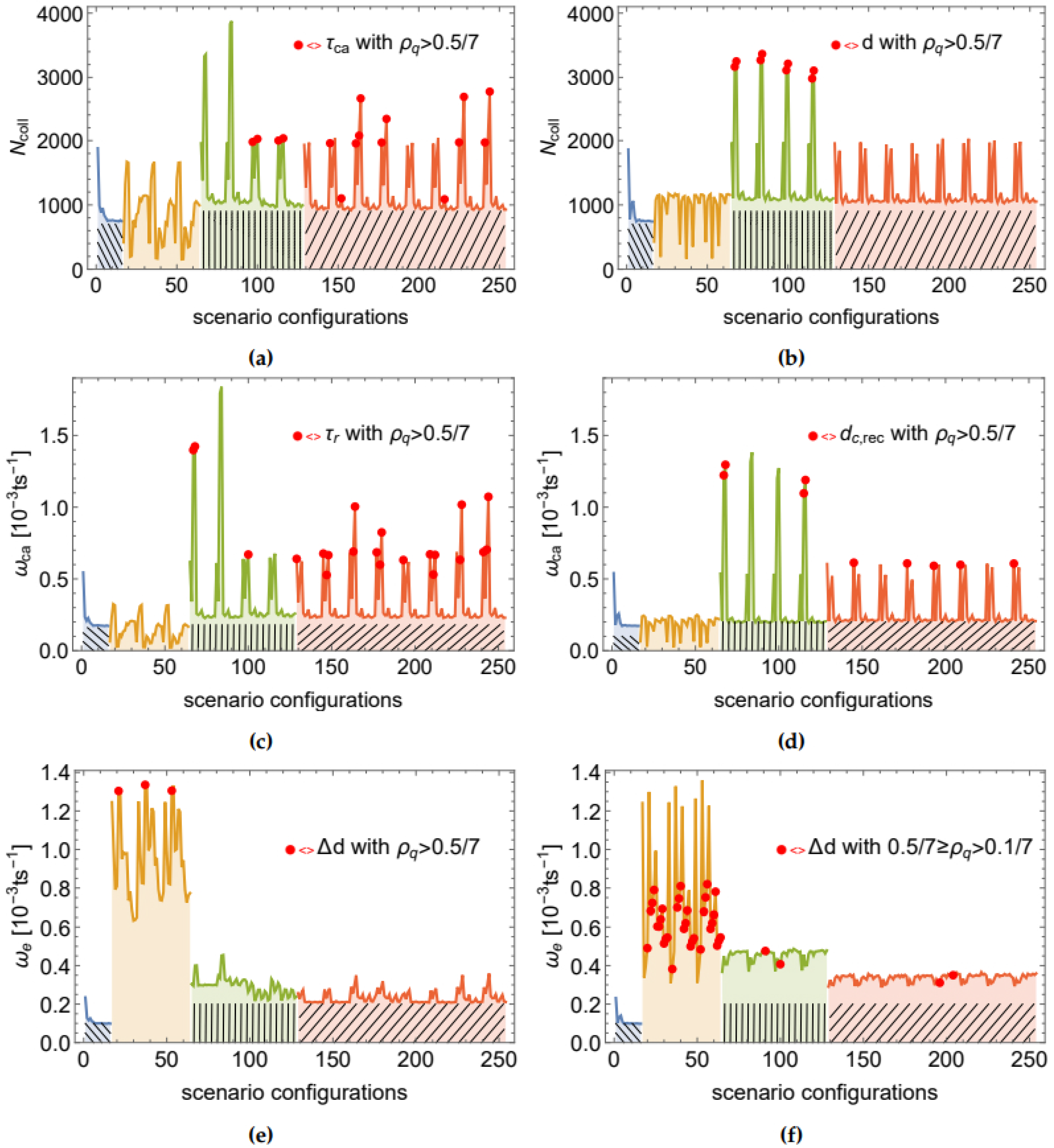
Figure 3 shows the values recorded for these three metrics under both continuous and DCMs and for the entire range of 256 scenario (cues) configurations, respectively. Repeating performance patterns can be observed over different sets of configurations. The regions over which these patterns emerge are (from left to right): (i) all scenarios with
and
, i.e., constant
(blue region with a left tilted mesh in
Figure 3), (ii) all scenarios with
and
, i.e., no social and only internal influence on
. This region is henceforth referred to as
(shown in orange, no mesh), (iii) all scenarios with
, i.e., low social impact on
(green region with vertical mesh, henceforth denoted as
), and (iv) all scenarios with
or
, i.e., high social influence on
(red region with right tilted mesh, henceforth denoted as
). Please note that in all four regions
is altered in the same way, i.e., for
and
all values from
are included. The best swarm performance in terms of
and
emerges when the influence of internal cues on the swarm dynamics is negligible compared to social cues, i.e., when
and
.
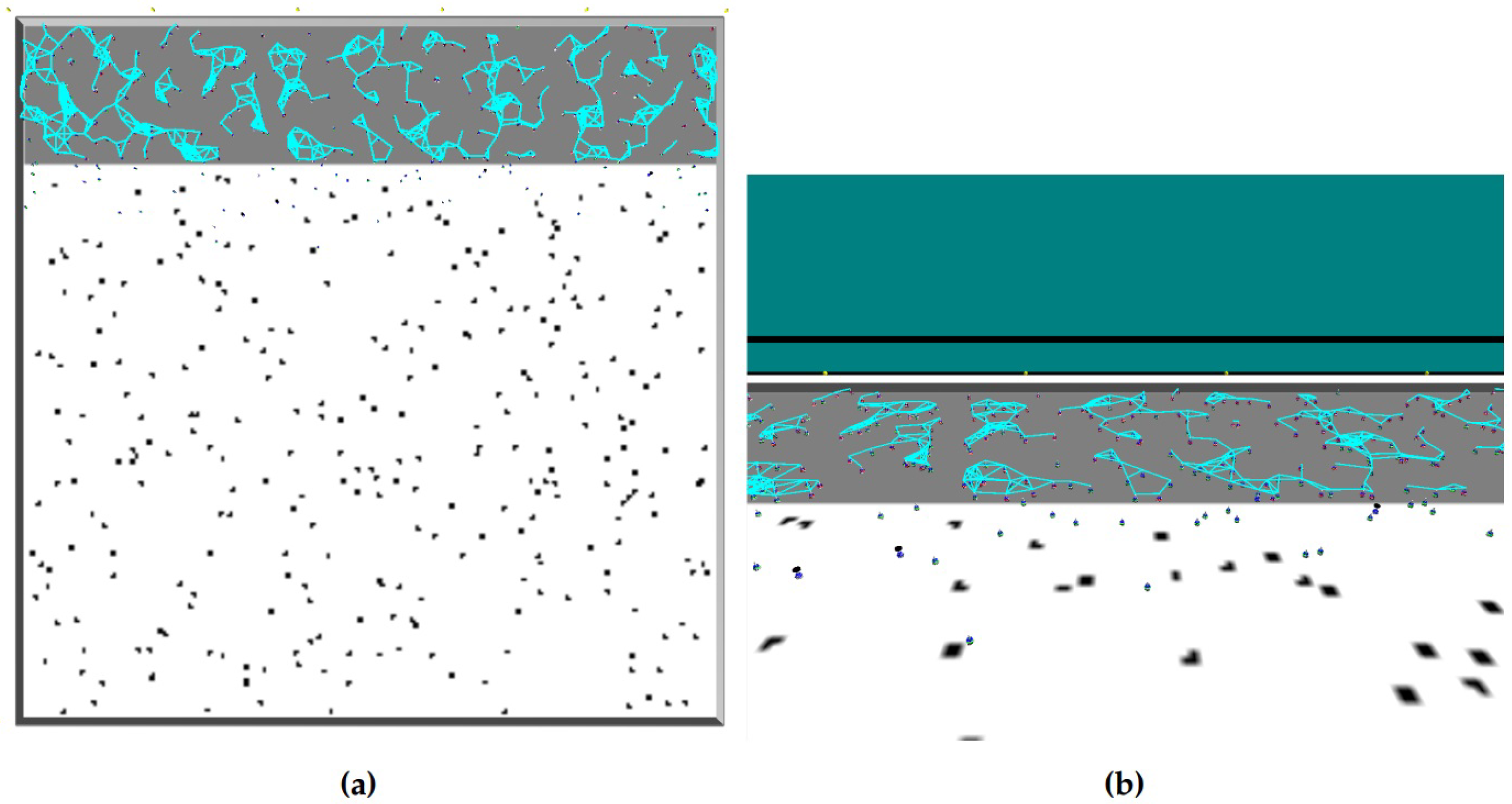
The best performance levels in terms of
and
were reached over the
region. For instance, the maxima of
and
correspond to the scenario configurations in which
,
and
. For the same configurations, (truncated) power law distributions of space features were found in the CCM (examples shown in
Figure 4). Contrary to CCM, in the DCM the robot interactions are interrupted. These interruptions may explain why, in DCM, space features such as communication degree tend to not follow a power law distribution (weak overall support for the presence of a power law behavior). Nevertheless, we found fits with moderate to strong support for (truncated) power law to time features, such as
and
, demonstrated in
Figure 5. The best power law fits of the DCM correspond to the peaks in swarm performance in terms of
and
over the
regions.
The third performance measure, i.e.,
, reached its best values over the
region. Its maxima correspond to cases where
and
. Interestingly, for these scenario configurations we found fits with moderate to strong support for (truncated) power law to the data of Δ
d, i.e., the change of the average communication degree of the robot (examples shown in
Figure 6). This is an interesting finding because it indicates that a communication feature may be power law distributed also in those scenarios in which the swarm tries to minimize the number of foraging robots and maximize the number of resting ones. Moreover, in most Δ
d distributions with strong or moderate support for the power law, the fit includes only 10–20% of data points. The reason for the relatively low ratio of power law fitted data is that the tail of the distribution is likely to represent by the fraction of robots that rest or move close to the border between the nest and the foraging area.
In general, the findings suggest that internal cues (in the absence of social cues) keep robots at the edge of minimal activity while social cues (in the absence of internal cues) drive the robots towards maximal activity.
3.2. Correlation with Swarm Performance
In the previous section we have illustrated that swarm performance is likely to reach its peaks over cue configurations that include asymptotically scale-free space or time features (see
Figure 3). In this section, we analyze this observation statistically, using correlation measures such as the Pearson and Kendall’s tau rank correlation coefficients introduced in
Section 2.4.3. However, note that both correlation measures have strengths and shortcomings. On the one hand, while the Pearson correlation coefficient is widely used and has an elegant mathematical form, it is sensible to outliers and may not be appropriate for non-linear distributions. On the other hand, Kendall’s tau is suitable for non-linear distributions as well as robust to outliers. Nevertheless, reducing the values to ranks may disregard the significance of the variable’s value being far from the average. In particular, replacing the real value of the quality ratio
by its rank leads to loss of information about the extent to which
represents the quality of the power law distribution. Moreover, following the definition of Kendall’s tau in Equations (
11)–(
15), each difference between data point pairs is assigned the same weight which may not always be appropriate. For instance, consider the ranked swarm performance in terms of
and the corresponding distribution of
in CCM for
d in
Figure 7a and for
in
Figure 7b, respectively. In both cases, Kendall’s tau defined by Equations (
11)–(
15) returns values indicating no correlation (i.e.,
and
, respectively). However, as evident in
Figure 7, both cases show different dynamics, with
for
d following
more closely than for
. The main reason is that the dominant fluctuations of
close to zero are assigned the same weight (i.e., rank step 1) as the more permanent increase of
for high values of
. Similar considerations hold for the other features and the DCM. To account for this type of behavior, we use a generalization of Equation (
15) that weights the ranking steps by a parameter
, which is relative to the average change, such that:
and similarly, for
and
. The weight parameter
is given by
where
and
are averages over all
and
, respectively. For each
pair, Equation (
16) considers the data distances of both distributions, normalized by their respective mean distances. Consequently,
does not favor any distribution and weights each ranking step relative to other distances. Please note that in general, there is no correlation metric that is perfectly adequate for all types of studies and data distributions; it is thus common to consider appropriate modifications [
67,
68,
69,
70]. In the present case, for
we obtain the standard Kendall’s tau rank correlation coefficient described in
Section 2.4.3. However, by implementing Equation (
16), the correlation coefficient is less sensitive to fluctuations than the standard Kendall’s tau, while still being more robust to outliers and non-linearity than the Pearson correlation measure. Therefore, in the following we will use this modified Kendall’s tau rank correlation coefficient to investigate the presence of correlations between
and swarm performance.
The correlations are shown for all features in
Table 5 between the three measures of the swarm performance and the feature ’scale-freeness’ quantified by
. We found strong correlations of the scale-free property of various features with the swarm performance. In particular, high correlations exist for
, Δ
d in DCM; and, additionally, for
in CCM. Remarkably, for those features for which we found moderate or high correlation values (highlighted in blue in
Table 5), most high-quality power law fits appear in the same scenarios as the highest swarm performance peaks. The red dots in
Figure 3 illustrate this finding by highlighting the scenarios in which the quality ratio is
. Moreover, the swarm tends to demonstrate low performance with respect to
and
for those scenarios in which
is highest, the latter being well correlated with Δ
d.
The correlation coefficients confirm the observation, supported by the data shown in
Figure 2 and
Figure 3, that most power law distributions with strong support (i.e., high
) appear in scenarios with peak swarm performance. To further examine this observation, we consider the correlations of the swarm performance with different
support classifications (based on
Table 3). As
Table 6 shows, there are moderate and strong positive correlations between features with strong support for power law distribution and swarm performance in terms of
and
for both communication modes. This suggests that the observation of scale-free features is more likely in scenarios in which the agents are more successful in retrieving a high number of food items.
3.3. The Role of Feedback Mechanisms in the Emergence of Scale-Free Features
An attribute of complex systems that is widely known to support the emergence of scale-free characteristics is the presence of (positive and negative) feedback loops [
1,
53,
71]. We specify the feedback effect to be positive or negative based on the individual response to the information input from its neighborhood. Hence, we refer to the feedback mechanism as
positive feedback if it pushes the individuals to the same state as the state of the majority, whereas
negative feedback pushes them away from it.
Most scale-free features were found in scenarios in which (i) the robot behavior was dominated by social interactions, (ii) the swarm attempted to balance positive and negative feedback and (iii) the swarm displayed a tendency towards active exploration. In particular, in CCM, the first 17 scenarios sorted by in descending order were found over the region and with . Similarly, in DCM, the first 28 scenarios were found over the region and with . To understand this, it is necessary to consider in more detail the impact of each cue on swarm dynamics and the feedback mechanisms.
For conciseness, we focus our system analysis on CCM and its most relevant set of parameter configurations. Similar conclusions hold for DCM. In particular, we can simplify our analysis based on the repeating patterns of swarm performance (see
Figure 3) and the following observations: (i) The swarm performance is qualitatively very similar between the cue values 0.5 and 0.9 (for all four cues). Thus, we focus, in the following, on
. (ii) The cue
has a negligible impact on the foraging dynamics when
. By neglecting scenarios in which
, except those with
, we can further shorten the set of relevant scenarios. Finally, (iii) there are significant differences in the dynamics between scenario configurations with
and those with
but negligible differences between
and
. Thus, we focus, in the following, only on scenarios with either
or
.
Figure 8 shows the final set of 24 scenarios relevant to the discussion below.
Please note that (ii) and (iii) are consequences of the internal cues and acting only on exploring robots. In the exploring state, the crucial parameter is because it defines the probability to stop exploring and change to resting. A non-zero value of the internal cue has a substantial impact on dynamics as it alters after each exploration attempt. As the likelihood of finding and retrieving a food item is low, mostly reduces . The more is lowered by , the less likely the robot is to find a food item during the next exploration attempt. Thus, has a strong inhibitory influence on the swarm’s exploration activity. Consequently, there is a significant difference in swarm performance between the scenario configurations with and those with . As the swarm actively attempts to explore the environment and collect food items, the influence of can be considered an important driver of negative feedback. In contrast, acts only on resting robots. Consequently, any change of through is easily distorted by , i.e., the social interactions with the neighborhood of the resting robot. Hence, only when there is an inhibitory impact of on swarm dynamics (similar to , due to the scarcity of food items), otherwise is negligible. In short, when the probability of finding a food item is low, with and enabling the swarm to significantly damp the feedback mechanisms that drive the swarm towards inactivity.
Next, we consider the particular contributions of social cues and . Social interactions represent a direct form of feedback loops, enabling the swarm to drift towards an absorbing state (e.g., uninterrupted resting or exploring) or maintain a balance between positive and negative feedback. In general, note that high values of often lead to due to the high probability of encountering a robot with a failed exploration (due to the low density of food items). With such relatively high values of , can be reduced to zero within a few time steps. By contrast, with , does not fluctuate as strongly. Similar considerations hold for and . In terms of active exploration, i.e., long exploration times and high number of retrieved items, it is beneficial for the swarm to have robots with and . Indeed, in the present system we observe that the swarm approaches such behavior for and (i.e., over the region). More importantly, such balance of and allows positive and negative feedback loops to coexist with the positive feedback being slightly more dominant. Due to this feedback coexistence, a robot that happened to be surrounded by unsuccessful neighbors will tend to have low and high , i.e., its resting time will increase (together with its d or ) and vice versa. Over time, such dynamics will result in robots that are increasingly inactive (with increasingly higher , d or ) and robots that are increasingly active (with increasingly lower , d or ). When the majority tends towards active exploration, the inactive group of robots experiences negative feedback and while the active group is subject to positive feedback. The prevalence of the positive feedback decreases the number of consistently resting robots significantly below the number of consistently exploring ones. Ultimately, this leads to skewed or heavy tailed distributions, such as the power law and, consequently, to the emergence of scale-free features. Similar considerations apply to the DCM over the region. The difference is that in DCM each robot can broadcast its exploration result only once. Thus, needs to have high values for dynamics similar to CCM to emerge.
To illustrate the above considerations, let us examine the scenario configuration of CCM with
,
,
, and
(see
Figure 4a), in which a high performance value of
was observed (i.e., this scenario is similar to the peak in
Figure 8). The value of
has a high impact on
(the probability to transition to resting). For example, if a robot receives at least two ‘success’ messages more than ‘failure’ messages—i.e., if
in Equation (
2)—its
drops to zero. When
and
, the robot will stop exploring only if it finds an item. During the subsequent resting, this robot is likely to cause one of its neighbors to reach
, which repeats an analogous cycle of events. The corresponding dynamics can be translated in terms of the positive feedback pushing the robots out of the nest and increasing the number of robots in the foraging area (i.e., in the exploring state). In the long term, due to the positive feedback, the swarm drifts towards the absorbing state in which all robots have
and
. In the short term, while most robots is exploring, some robots remain in the nest, e.g., due to crowding at the entrance of the nest. Those robots have a higher number of neighbors because the nest is significantly smaller than the foraging area. Therefore, during this crowding behavior, the swarm experiences the coexistence of positive and negative feedback loops. A specific balance between these feedback loops may lead to the emergence of scale-free features such as the space feature
d (for which, indeed, the above mentioned scenario configuration has one of the best truncated power law fits with
, shown in
Figure 4a). Similar considerations hold for other CCM examples presented in
Figure 4 or the DCM examples in
Figure 5.
The above example demonstrates positive feedback regarding the
exploring state. However, under some configurations, positive feedback can also be observed around the
resting state. For example, during the crowding behavior in the nest, a robot which is surrounded by a high number of resting neighbors is likely to get ‘stuck’ and be unable to leave the nest. This robot will eventually switch to the resting state and broadcast a ‘failure’ message. Neighbors that receive this message will decrease their probability to explore
, and, through physical interference, lower the neighboring robots’ chances to leave the nest. Consequently, positive feedback at the resting state may lead, in the long term, to an increase of the average communication degree of the resting robots and the emergence of power law distributed features, alongside the occurrence of outstanding robots whose features such as Δ
d (examples shown in
Figure 6),
or
exhibit exceptionally above-average values.


