A New Modeling Method of Angle Measurement for Intelligent Ball Joint Based on BP-RBF Algorithm

Abstract

The rotation orientation and the angle of precision of an intelligent ball joint cannot be automatically obtained in passive motion. In this paper, a new method based on a Hall sensor with a permanent magnet (PM) is proposed to identify the spatial rotation orientation and angle. The basic idea is to embed a PM on a ball while the Hall sensors are arrayed into the ball socket. When the ball rotates, the Hall sensor array detects the variation of the magnetic induction intensity in space. By establishing a mathematical model between the variation of the magnetic induction intensity and the orientation and angle of rotation, the rotation angle in the space where the ball is located can be inversely solved. The establishment of the theoretical model is based on the theory of the equivalent magnetic charge method, which has a few native defects that cannot be overcome by itself. This paper presents the relationship between the magnetic induction intensity change and the rotation angle of the ball in space, which was constructed by an artificial neural network (ANN) and will simplify the mathematical model, shorten the operation time, and improve the efficiency of real-time detection. Based on the simulation analysis, the optimal matching scheme between the PM and the magnetic effect sensor was determined, and the structural parameters of the ball joint prototype were optimized. The data training and comparison test of the neural network model were completed on a self-developed calibration device. The experimental results show that for a ±20° measurement range, the average errors of the uniaxial measurements are 1′51″ and 1′55″ on the two axes, respectively. At present, the measurement accuracy of the prototype is still relatively low; however, this idea of modeling based on ANN removes the shackles of mathematical modeling, reminding us that we can consider the design of sensors or complete geometric measurement modeling from a new perspective.

1. Introduction

Precision ball joints are widely used in parallel robots and measuring instruments, however, they cannot automatically acquire their orientation in space. With the support of the National Natural Science Foundation of China, we have developed a method to measure the rotation angle of a precision ball joint. As shown in Figure 1a, a permanent magnet (PM) was embedded on the ball and a Hall sensor array was arranged in the ball socket. When the ball rotates in any direction with the rod, the PM will also rotate around the ball center, resulting in a variation of the magnetic induction intensity component. The angle of rotation about the X-axis is given by α, while that about the Y-axis is given by β. The Hall sensor array captures the variation. Based on the equivalent magnetic charge method (EMCM), a measuring model between the reading of the Hall sensor and the rotation angle in the space of the ball joint was established. Figure 1b shows the first prototype [1,2].

The modeling process based on the EMCM is shown in Figure 2. The basic coordinate system O-XYZ was established with the ball center as the origin O and the axis of the ball joint as the Z-axis vertically upward. The ball moves from the initial position M to M’. The rotational motion of the ball in the ball socket can be decomposed into a rotation angle around the X-axis and a rotation angle around the Y-axis. At this time, the dynamic coordinate system O-X’Y’Z’ was established with the ball center as the origin and the axis of the ball joint as the Z-axis vertically upward.

As shown in Figure 2, the three Hall sensors S₁, S₂, and S₃ were placed in the ball socket. Taking one sensor S₁ as an example, the modeling process based on the EMCM is described. It is supposed that the coordinates of S₁ are (x₀, y₀, z₀) in the base coordinate system and (u, v, w) in the moving coordinate system. In the latter system of O-X’Y’Z’, using the EMCM, when the ball rotates from the initial position M to M’, the magnetic induction component at the position of S₁ can be expressed as B_M’ = (B_x’, B_y’, B_z’). According to the coordinate transformation formula, the three-dimensional component of the magnetic induction intensity at the position of S₁ in the moving coordinate system O-X’Y’Z’ can be converted to the three-dimensional component in the basic coordinate system O-XYZ.

$$\{\begin{array}{c}{B}_x=B_x{}^{\prime }\cos \beta +B_z{}^{\prime }\sin \beta \\ B_y=B_x{}^{\prime }\sin \alpha \cdot \sin \beta +B_y{}^{\prime }\cos \alpha -B_z{}^{\prime }\sin \alpha \cdot \cos \beta \\ B_z=-B_x{}^{\prime }\cos \alpha \cdot \sin \beta +B_y{}^{\prime }\sin \alpha +B_z{}^{\prime }\cos \alpha \cdot \cos \beta \end{array}$$

(1)

where B_x, B_y, and B_z are the magnetic induction components of the sensor in the base coordinate system and B_x’, B_y’, and B_z’ are the magnetic induction components of the sensor in the moving coordinate system; α and β are as previously defined.

The three Hall sensors were placed horizontally on the prototype and their magnetic induction values are their axis directions. Under the basic coordinate system O-XYZ, the magnetic induction intensity values measured by Hall sensors at the position of S1 are the composite values of the magnetic induction intensity in the direction of X-axis and Y-axis, which can be expressed as follows:

$$B_{S_1}=B_x\cos \delta +B_y\sin \delta$$

(2)

where the angle between the sensor axis and the X-axis is δ and the value of δ₁ at S₁ is 90°.

The relationship between the field values measured by S₁ and the rotation angles α and β can be obtained using the Equations (1) and (2) simultaneously, which are expressed by Bs₁ = f_S1(α, β). Similarly, Bs₂ and Bs₃ can be obtained. Theoretically, setting two Hall sensors is sufficient for constructing equations and obtaining the angles α and β. Here, three Hall sensors were employed redundantly, which is helpful to improve the accuracy and stability of the measurements.

Through the experiment comparison and a test, the measuring error of the developed prototype based on the EMCM model was determined; the average errors were 16 min within a 10° measuring range, and 29″ within ±20° [3,4].

The theoretical and experimental results show that the mathematical model established by the EMCM has a higher accuracy for a small-angle range. However, the theoretical model requires strict structural parameters of the PM and assembly accuracy of the Hall sensor, while the calculation accuracy decreases with increasing measurement range. In addition, according to the mathematical model established by the previous research of the project team, the calculation takes a lot of time to iterate as the model contains multiple integrals. This is not leading to the real-time monitoring of the rotation angle of the ball joint. Therefore, we hope to find and update the model methods [5].

An artificial neural network (ANN) is a numerical modeling method by training and learning, which completely abandons the analytical modeling used in sensors. Its calculation time is very short due to its simple structure. In the meantime, its robustness and adaptability make it insensitive to the mechanical structure parameter error of the ball joint, the residual magnetic deviation of the PM, and the manufacturing and assembly error. We expect to replace the complex mathematical model with the ANN algorithm [6].

2. Simulation Analysis of Artificial Neural Network (ANN) Modeling

2.1. Selection of ANN

We used the EMCM model to first construct theoretical training data, which was then used to complete the learning and training of the ANN. According to the results of the simulation analysis, the types and technical parameters of the specific ANN algorithm will be achieved.

MATLAB was employed to program and simulate the analysis. As Back Propagation (BP) ANN has a strong nonlinear mapping ability, flexible network structure, simple theoretical basis, and wide application range, it was used to first partition the training data. After data classification, the Radial Basis Function (RBF) ANN was used to fit the relationship between the magnetic induction intensity and the rotation angle in the space of the ball joint [7,8,9]. RBF ANN was chosen because it can approximate any nonlinear function with arbitrary accuracy and has the unique best approximation characteristic [10,11,12]. At the same time, its learning rules are simple and its convergence speed is fast.

2.2. Simulating Realization of ANN

For the simulation calculation, the input of the ANN was the theoretical reading value of the Hall sensors, while the output was the rotation angle components α and β in the space of the ball joint. The purpose of simulation is to determine the number of suitable input terminals of the artificial neural network so as to minimize the measurement error. According to the data training process of the ANN, the specific simulation steps are:

• In the measurement range of [−20~20°], the output magnetic induction intensity of the Hall sensor collected at intervals of one unit acted as the input of the ANN to build the model, while the angle corresponding to (α,β) was used as the output of the ANN to build the model. Because the sigmoid function is sensitive to the slight changes in the middle and the recognition degree of ANN is better, the sigmoid function was used to scale the data into the interval [−1,1].
• According to the training rules of the ANN, the initial parameters (W,b) of the ANN were arbitrary numbers in (0,1), whether the W and b represented all weighting matrices and bias vectors in ANN, respectively. The output of the first training (α₁,β₁) was calculated, then the parameters (W,b) were updated according to the function of the ANN itself. After several iterations, the parameters of ANN (W,b) which minimized the error output function were obtained.
• When all the training data of the neural network were finished and the output error was minimized after simulation, and the output achieved the required accuracy, the ANN modeling was complete.

Two problems must be solved in the simulation. The first concerns the suitable number of input terminals of ANN. The second is how to choose the number of hidden layers of the ANN to improve the measurement accuracy. When the number of input terminals of ANN is three to five, the calculation error of the model is as shown in Figure 3. The angle components α and β have similar error characteristics, so, the figure only lists the error values and law of the simulation measurement of angle α. The output error of the BP ANN is observed to decrease with the increase of the input. When the number of input terminals of ANN reaches five, the error no longer decreases. Similarly, we simulated the effects of the number of hidden layers on the calculation error and measurement accuracy of the model. Figure 4 presents an error diagram of the angle component α of the BP ANN with multiple hidden layers when the number of sensors is constant. As can be seen, increasing the number of hidden layers reduces the output error. When increased to four layers, the calculation error tends to be flat. Finally, the BP ANN adopts the structure of five inputs and four hidden layers [13,14,15,16].

The simulation results show that the RBF ANN has a good nonlinear mapping ability and a fast convergence speed. The design of the hidden layer of the RBF ANN determines the number of the cores in the hidden layer. The RBF ANN trains and learns in [−20°~20°], so too many kernels will reduce the iteration speed and the curve approximation ability [17]. The measurement interval was divided into four parts using the BP ANN: The first interval was 0° ≤ α ≤ 20°, 0° ≤ β ≤ 20°; the second interval was 0° ≤ α ≤ 20°, −20° ≤ β ≤ 0°; the third interval was −20° ≤ α ≤ 0°, 0° ≤ β ≤ 20°; the fourth interval was −20° ≤ α ≤ 0°, −20° ≤ β ≤ 0° (as shown in Figure 5). In each interval, the magnetic induction intensity values (B₁, B₂, B₃, B₄, B₅) at the positions of the three sensors (two unidirectional and 1 three-directional) were used as the input of the training data. The (α,β) angles constructed by the EMCM were taken as the output of the training data of the RBF ANN. The input and output were substituted by the RBF ANN for learning.

The K-means clustering algorithm is a widely used unsupervised clustering learning algorithm. It accepts K inputs, and then divides n data objects into K clusters to satisfy the clustering. According to the workflow of the K-means clustering algorithm, the K-means algorithm was used to determine the number of kernels in each interval. To determine the number of cluster kinds in the K-means algorithms by stepwise approximation: Firstly, when k = 30, 60, 90, 121, the K-means algorithm was used to train the descendants in the RBF network, and the minimum output error K₁ was selected. Comparing the clustering results of k = k₁ + 30, k₁ − 30, k₁ + 20, k₁ − 20, and then reducing the range of k values according to the output error of the network, the optimal k value can be obtained. The matrix dimension of W was determined by the number of core centers [18]. At the beginning, the random (W,b) parameters were obtained. The training process was similar to that for the BP network. After the calculation, the k values of the first to the fourth intervals were 55, 41, 121, and 41, respectively. The angular errors of the RBF ANN in each interval are shown in Figure 6. The errors of angles α and β are similar, thus, only the errors of angle α are listed in the figure. The angle error values of one to three intervals are similar, and the angle error values of the fourth interval are relatively minimal. This is because the K-means algorithm has the characteristics of local optimal solution. Because of the high fault tolerance of ANN, the error has little effect on the modeling of ANN.

Generally, after the experiments and tests, the BP neural network is selected to partition the test data. Meanwhile, the RBF neural network fits the relationship between the magnetic induction intensity measured by the Hall sensor array and the rotation angle in the space of the ball joint.

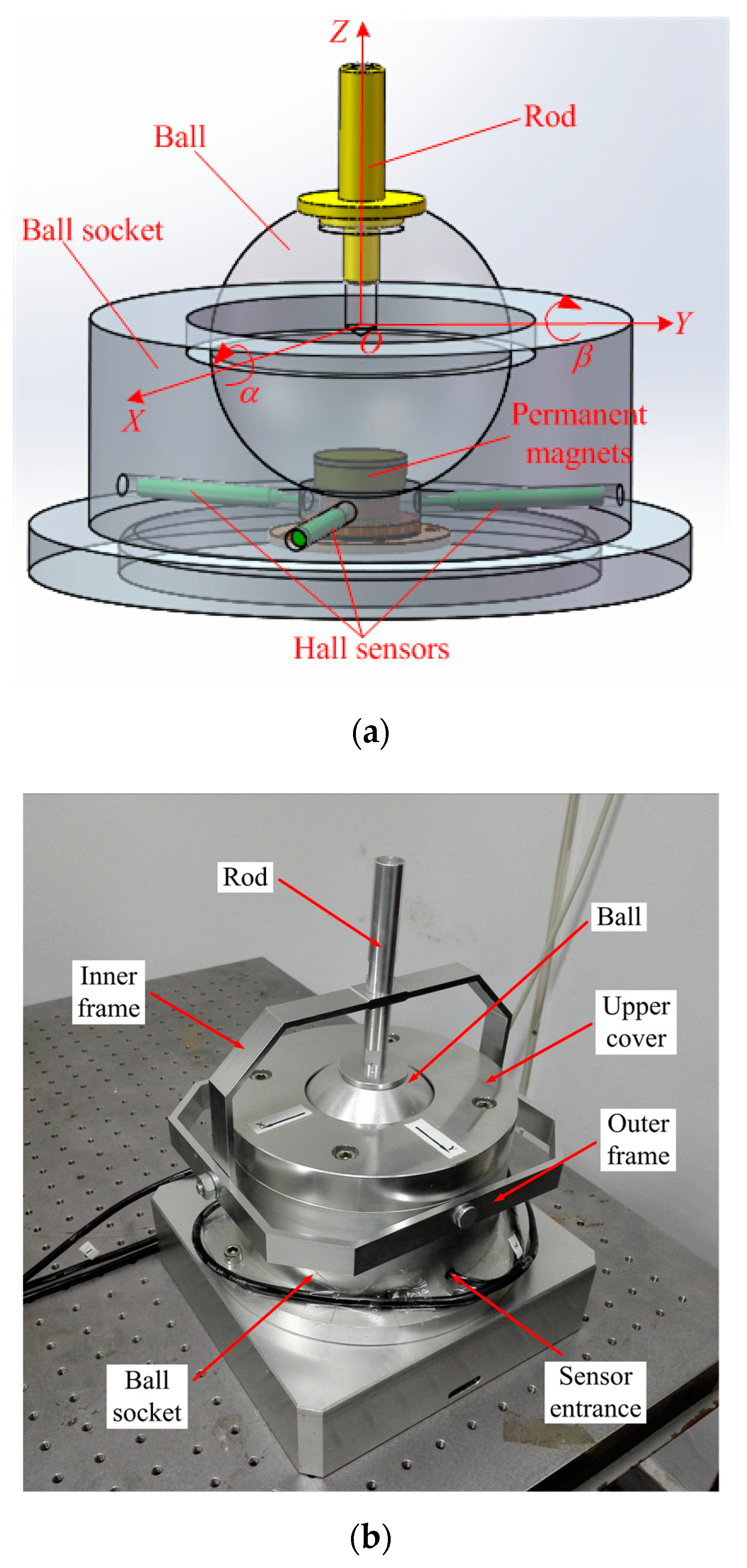
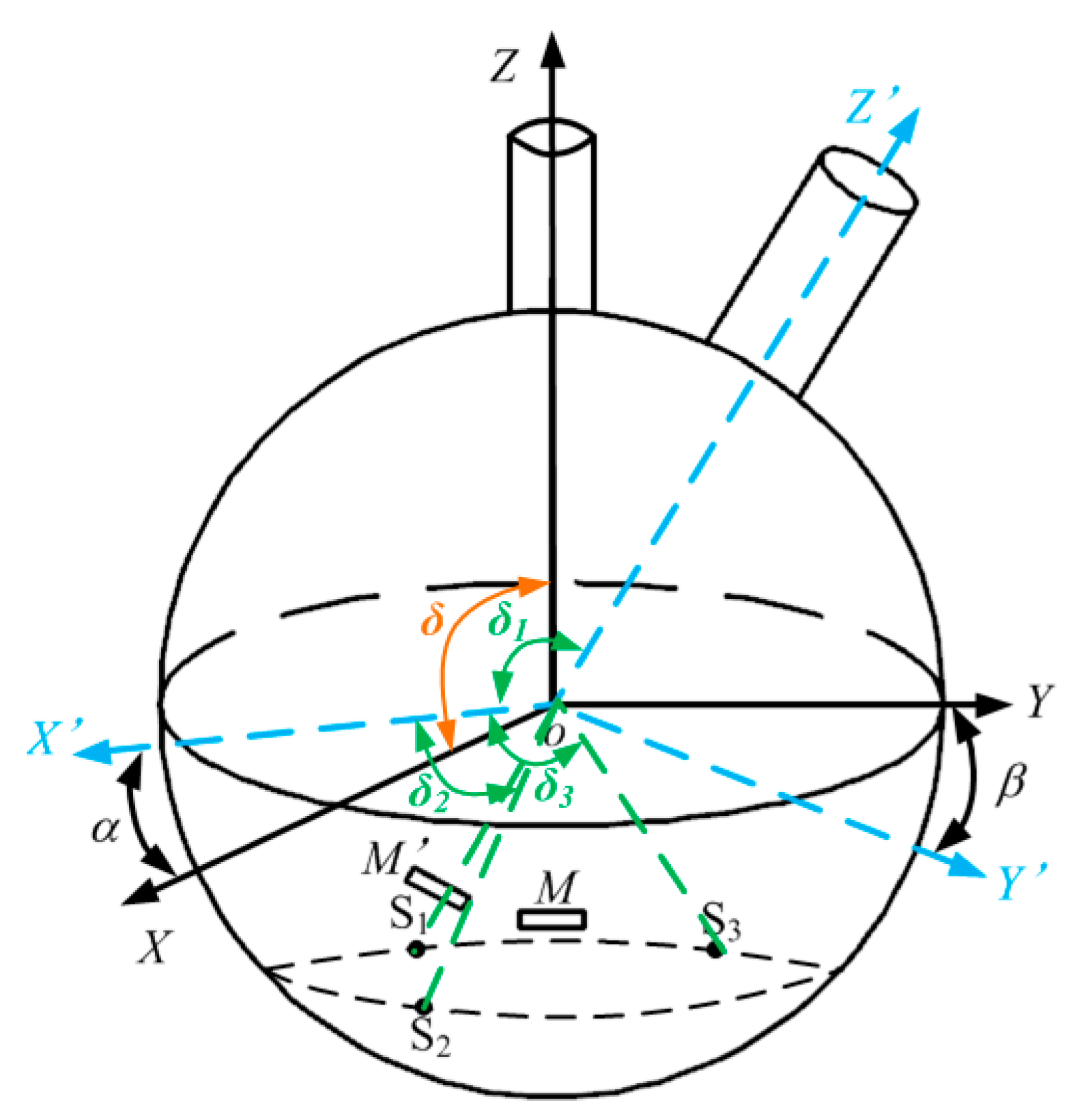
3. Prototype Development

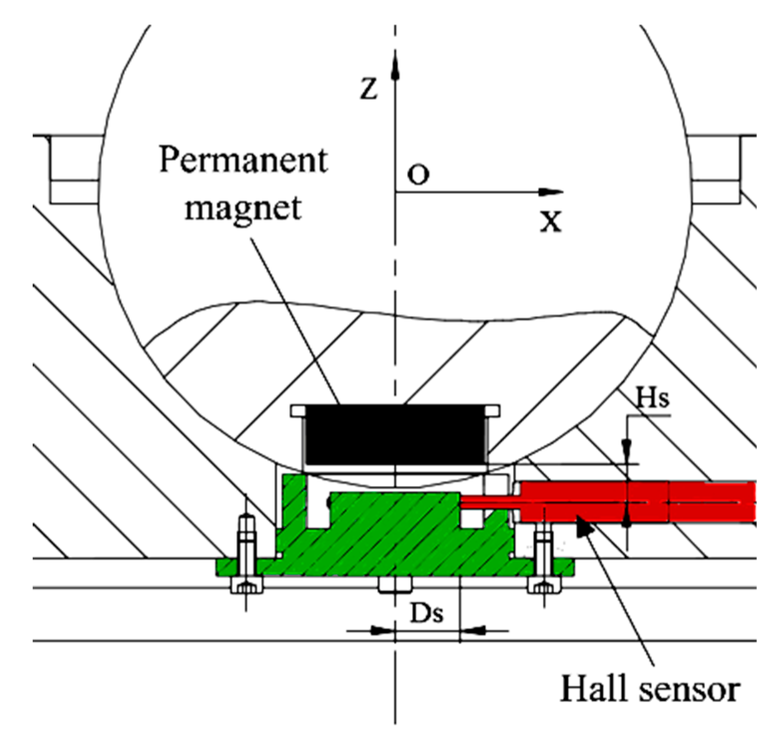
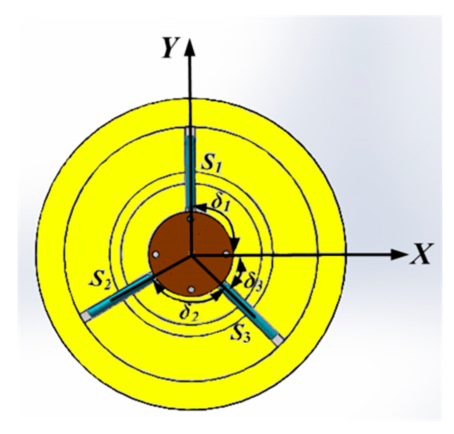
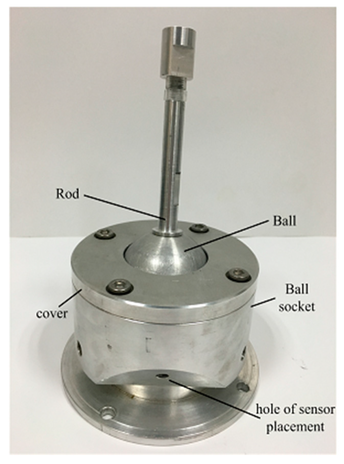
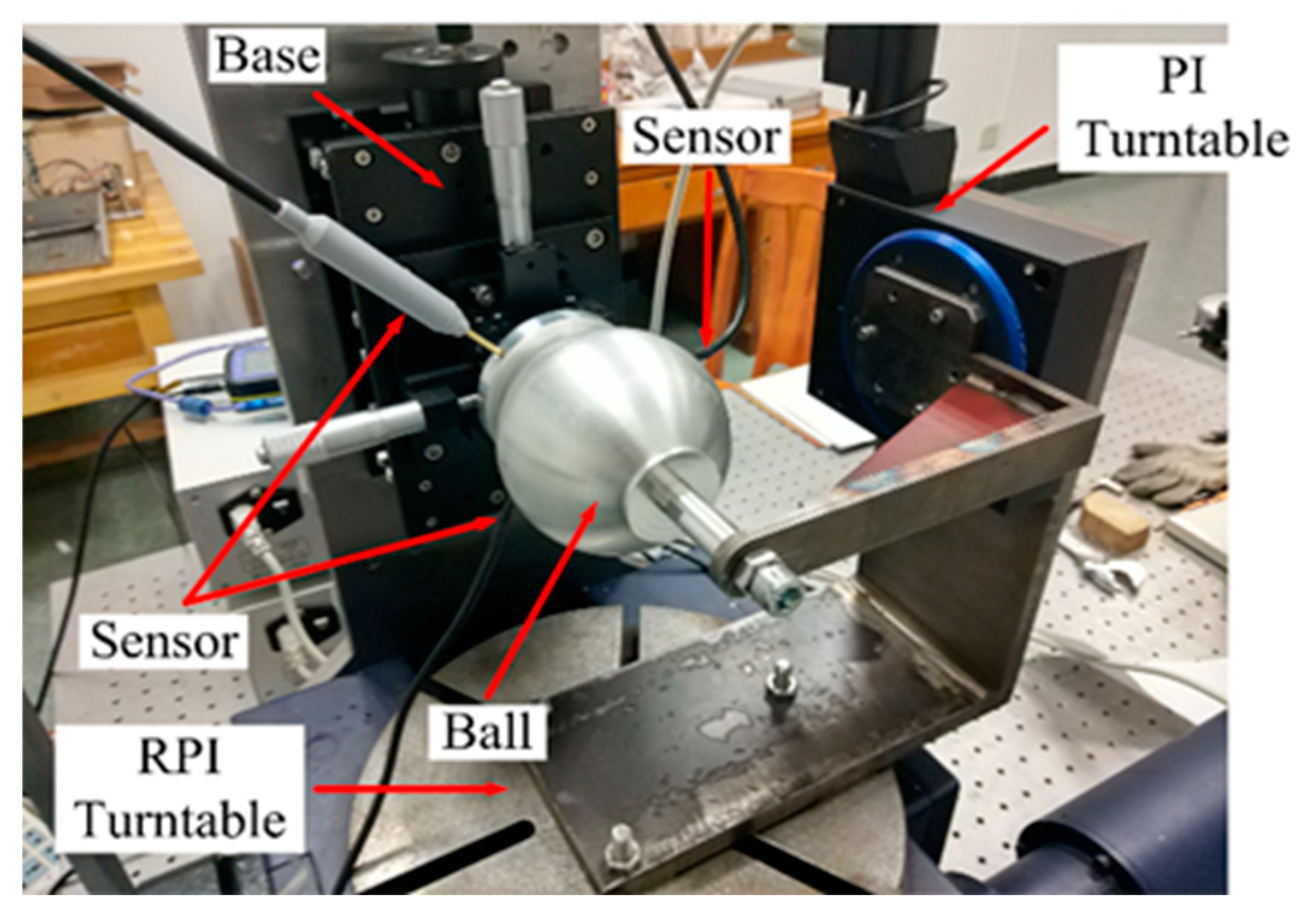
3.1. Design of Mechanical Part of Measuring Prototype

Based on the above simulation results and experience from the first prototype, the number of input terminals of ANN was five. After evaluation and comparison, three Hall sensors were employed in the new prototype: two single-axis sensors (CH1600, Beijing Cuihai Jiacheng Magnetoelectrics Technology Co., Ltd, Beijing, China) and one three-axis sensor (MZ-530A, Beijing Cuihai Jiacheng Magnetoelectrics Technology Co., Ltd, Beijing, China). According to the characteristics of the ANN, the PM was redeveloped by Maxwell simulation analysis, that is, a cylinder with a radius of 15 mm and a height of 10 mm. The relative permeability was 1.1 and the remanence parameter Br was 1200 mT.

The key part of the new prototype is shown in Figure 7. The relative positions of the permanent magnet and the Hall sensor were determined by two main parameters. Assuming that the distance between the sensor axis and the lower end face of the permanent magnet in the Z-axis direction is given by Hs, the sensor detects the distance between the end face and the axis of the permanent magnet in the X-axis direction, given by Ds. The different values of Ds and Hs make the change trend of the magnetic induction intensity of sensor detection different. Without exceeding the ball joint detection range, the more drastic the change in the magnetic induction intensity value detected by the sensor, the more conducive to improving the accuracy of the solution of the neural network. A special round fixture was assembled on the bottom of the joint house. Three Hall sensors were distributed around the fixture cylinder surface, their heads attached on a cylindrical surface with a diameter of Ds = 12 mm. The position at this time did not affect the movement of the ball in the ball socket and facilitated the positioning and assembly of the Hall sensor in the prototype. The assembly size of Hs = 6 mm was optimized to ensure the relative position between the PM and Hall sensor probe. As shown in Figure 8, in the base coordinate system, the angles of the three Hall sensor probes and the X-axis were δ₁ = 90°, δ₂ = −120°, and δ₃ = −45°. An image of the new type of ball joint processing is shown in Figure 9.

The size of the prototype is 230 × 220 mm and the radius of the ball is 50 mm. The material of the prototype is pure aluminium because of the principle of magnetic effect. The prototype consists of a rod, an upper cover, a ball, and a ball socket. The ball joint is connected with other moving parts through internal threads. The ball rubs and rolls in the spherical socket to complete spatial rotation. Its range of motion is from −20 to 20°.

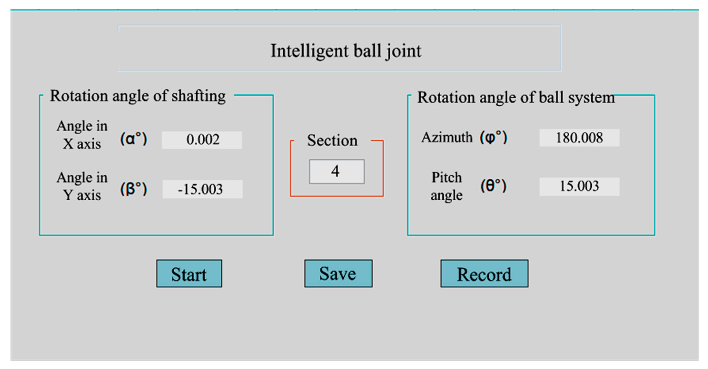
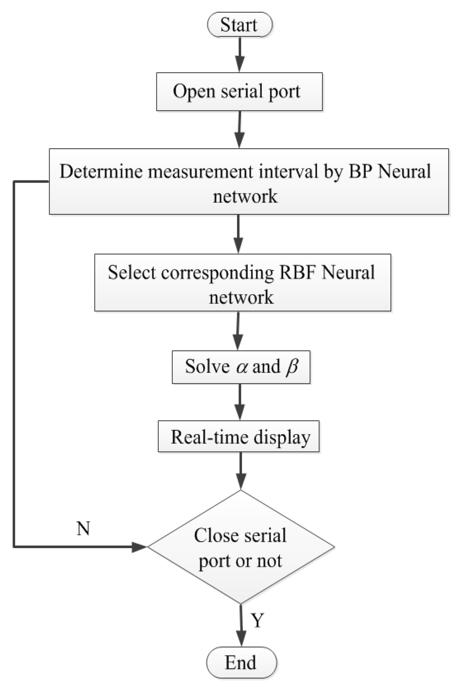
3.2. Design of Measurement Software

The measurement software was designed based on Python language. We used the wxPython graphics library (python 3.6 version, Python Software Foundation, Wilmington, DE, USA, 2016) to write the PC interface.

As shown in Figure 10, the interface includes the rotation angle (α,β) as well as the azimuth and elevation angles (φ,θ) in space. The interface is refreshed every 0.1 s. The main loop of the whole algorithm program detects whether the corresponding button is pressed. If the record key is pressed, the current rotation angle value of the interface will be recorded; if the save key is pressed, the record angle value is saved in Excel form. When the measurement is completed, the designed end button can interrupt the serial communication between the Hall sensor and the PC, and it can stop the real-time display function.

A flowchart of the upper software is shown in Figure 11. The flowchart runs as follows: First, when the upper computer program starts to run, it opens the PC serial port and sends a read–write signal to the Hall sensor. The Hall sensor returns the read magnetic induction intensity value, clearing the buffer data of the serial port every time it does so. Next, we enter the callback function, and use BP ANN to divide the read magnetic induction intensity into intervals. Finally, according to the interval, the five magnetic induction values read by the three Hall sensors are calculated by the corresponding RBF ANN, and the (α,β) values are obtained.

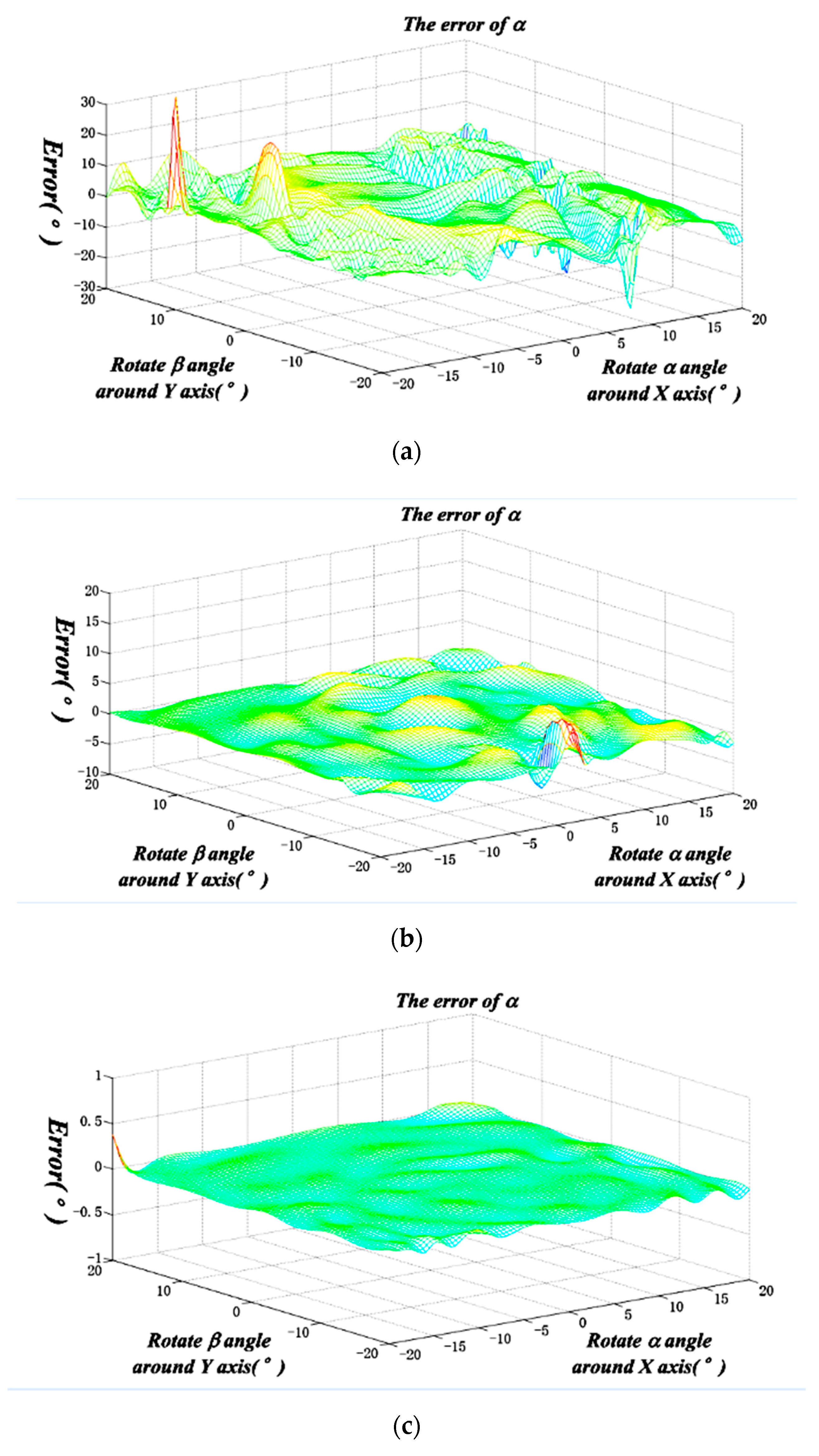
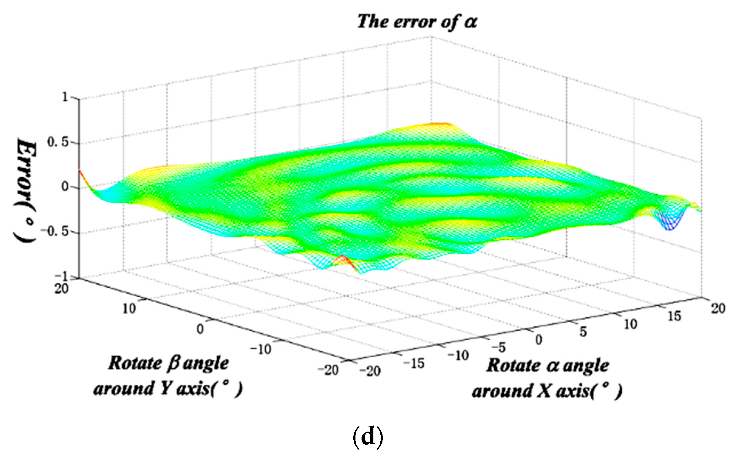
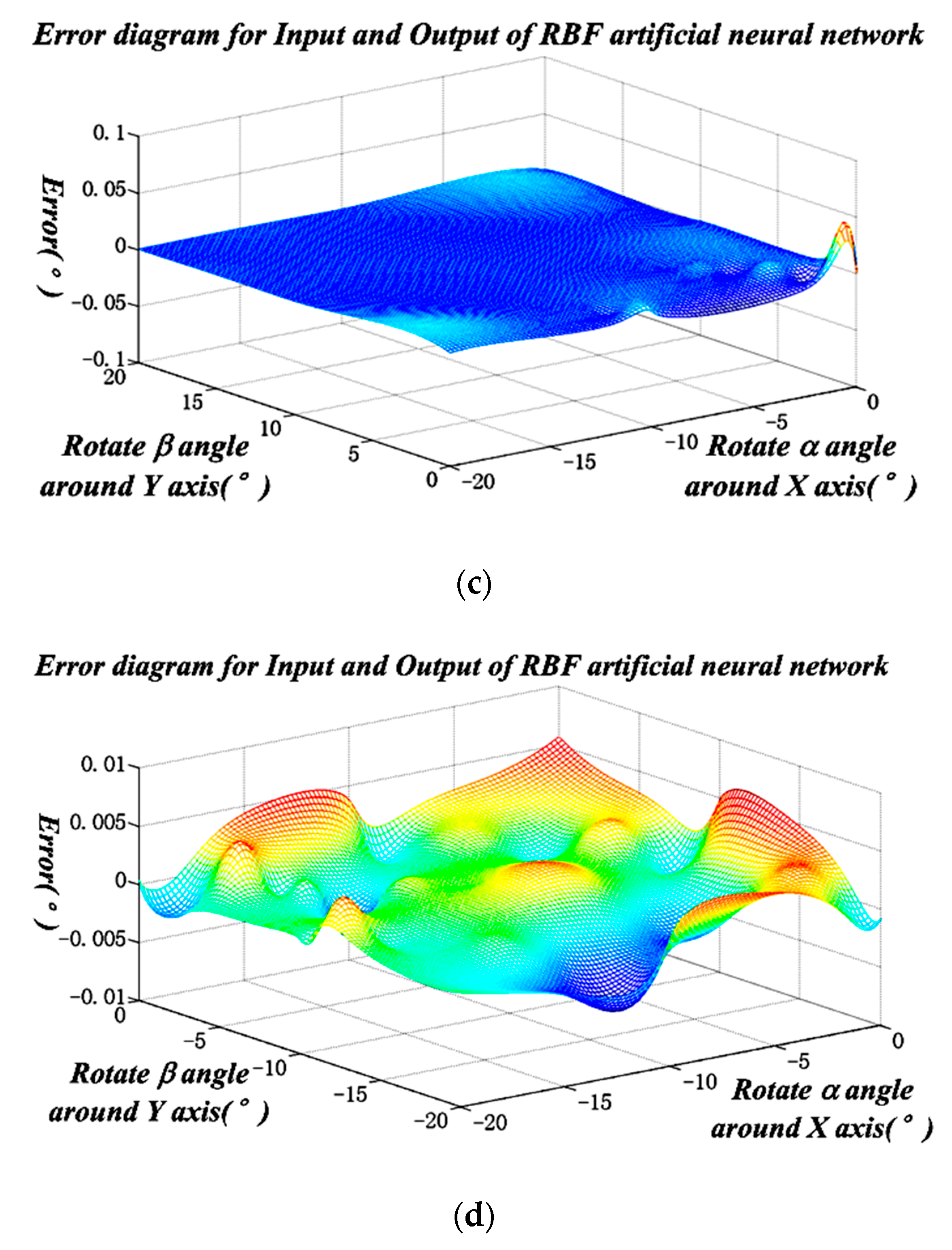
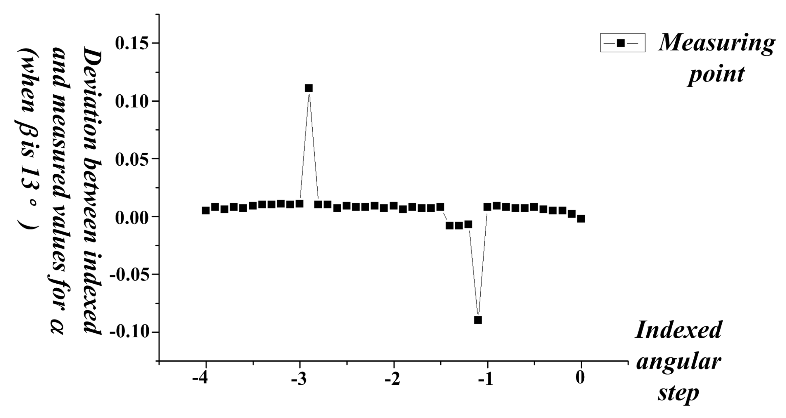
4. Training Modeling and Experimental Testing

Similar to the previous simulation analysis, the new prototype requires learning and training to complete the modeling process, that is, to establish the relationship between the five magnetic induction components and the rotation angle in the space of the ball joint. This process is completed on the biaxial angle self-developed calibration device.

The experimental process is shown in Figure 12. The M-060.DG angle encoder, of the PI company in Germany, provides a standard rotation angle α around the X-axis. The maximum permissible error of the platform is ±2″ and the smallest indexed angle incrementis is 0.02″. The DP300 rotary table, of the RPI Company in the UK, is used in the vertical direction. It provides the standard angle β. Its maximum permissible error is ±1″ and the resolution is 0.2″. To adjust conveniently, the ball socket is removed and three Hall sensor positioning fixtures are fixed directly on the three-dimensional stage. The three-dimensional stage comprises a vertical elevator and a two-axis horizontal displacement stage. The relative position between the Hall sensor and ball (or PM) is adjusted accurately by the microdisplacement mechanism at every stage.

During learning and training, the experimental device rotates the ball joint in any orientation, and it provides the standard angles of α and β stepwise at 1° intervals of rotation. At the same time, the computer records the angle value and the corresponding reading values of the five magnetic sensors, so the data samples can be obtained for training the BP and RBF ANN.

After modeling, the actual comparison measurement was still completed on the calibration device. As the β of −13° and the α from 0° to −4° are representative, these values were taken as examples. Firstly, the rotation angle β of the RPI controller around the Y-axis was unchanged at −13°, while α of the PI controller around the X-axis varied from −20° to 20° every 30′. The output angle value was compared with the indexed value from the PI turntables, the error of which is shown in Figure 13. The variation of the errors in each interval is not obvious. The maximum and minimum α errors were 7′58″ and −5′34″, respectively, and the average error was 1′44″. The maximum and minimum β angle errors were 6′18″ and −3′36″, respectively, and the average error was 46″.

The selection of α was similar to that mentioned above. The control angle of the PI displacement platform was fixed at 8°, and the control angle of the RPI displacement platform changed from −7° to 6°39′ every 36″. The output value of the intelligent ball joint was measured as shown in

Table 1. α changes with each 0.01°, the detection output value of ball joint.

Actual Value β (°)	Deviation Value β (°)	Actual Value β (°)	Deviation Value β (°)
−6.990	−0.005	−6.810	−0.003
−6.980	−0.005	−6.800	−0.004
−6.970	−0.003	−6.790	−0.004
−6.960	−0.002	−6.780	−0.004
−6.950	−0.003	−6.770	−0.005
−6.940	−0.003	−6.760	−0.006
−6.930	−0.004	−6.750	−0.006
−6.920	−0.006	−6.740	−0.003
−6.910	−0.006	−6.730	−0.003
−6.900	−0.003	−6.720	−0.004
−6.890	−0.003	−6.710	−0.004
−6.880	−0.004	−6.700	−0.004
−6.870	−0.004	−6.690	−0.004
−6.860	−0.004	−6.680	−0.004
−6.850	−0.006	−6.670	−0.005
−6.840	−0.005	−6.660	−0.005
−6.830	−0.006	−6.650	−0.006
−6.820	−0.004

. Within the range of measurement, the maximum value of the α angle error was 47″, the minimum value was 18″, and the average error was 32″. The maximum value of angle β error was −21″ and the minimum value was −7″ with an average error of −11″.

In summary, the angle errors calculated by the ANN refer to the range of ±20°, and the average errors of α and β are 1′51″ and 1′55″, respectively. Therefore, compared with the EMCM, the method of ANN improves the measurement accuracy of an intelligent ball joint system and reduces the measurement error. Therefore, the application prospect is broader.

5. Conclusions

A modeling method using ANN for ball joint rotation angle detection was proposed in this paper. The corresponding ANN algorithm and software were designed and equipped, and a new prototype was developed. The main conclusions include:

• The RBF ANN was used to construct the relationship between the input and output of the intelligent ball joint measurement model. According to the technical characteristics and requirements of the ANN, a new prototype of intelligent ball joint was rematched and developed.
• The BP ANN was used to divide the measuring space of the intelligent ball joint into four sections. The whole algorithm comprises the front-end BP ANN partition algorithm and the back-end RBF ANN calculation angle algorithm. It optimizes the number of inputs and hidden layers of the ANN, and it improves the calculation accuracy.
• The experimental data show that, compared with the traditional analytical model, the measurement accuracy of the intelligent ball joint is improved by using ANN. At the same time, the manufacturing accuracy requirement and the assembly of the ball joint are reduced, and the real-time performance of the measurement method is increased.
• Python language was used to compile the upper computer interface of the intelligent ball joint, which meets the training, learning, and modeling requirements in the measurement of a ball joint, and basically achieves the real-time display of the rotation angle. This study reminds us that in precision measurement or sensor development, it is not necessary to establish traditional analytical models, and various intelligent algorithms may be a new choice.

References

1. Hu, P.; Lu, Y. Measurement method of rotation angle and clearance in intelligent spherical hinge. Meas. Sci. Technol. 2018, 29, 6. [Google Scholar] [CrossRef]
2. Hu, P.; Wang, L. A measurement method for ball joint spatial rotation angle. Sens. Mater. 2015, 27. [Google Scholar] [CrossRef]
3. Yang, C.Y.; Yen, M.H.; Chou, M.T.; Huang, Z.J.; Chen, S.K. Non-spherical ball-socket joint design for Delta-type robots. Mechatronics 2017, 45, 21–25. [Google Scholar] [CrossRef]
4. Xu, C.D.; Jiang, S.Y. Analysis of Static and Dynamic Characteristic of Hydrostatic Spherical Hinge. J. Tribol. 2015, 137, 021701. [Google Scholar] [CrossRef]
5. Er, S.; Tez, M. Problems of artificial neural network. J. Surg. Res. 2017, 222, 225. [Google Scholar] [CrossRef] [PubMed]
6. Villarrubia, G.; Paz, J.F.D.; Chamoso, P.; De la Prieta, F. Artificial neural networks used in optimization problems. Neurocomputing 2018, 272, 10–16. [Google Scholar] [CrossRef]
7. Cıbuk, M.; Budak, U.; Guo, Y.; Cevdet Ince, M.; Sengur, A. Efficient deep features selections and classification for flower species recognition. Measurement 2019, 137, 7–13. [Google Scholar] [CrossRef]
8. Dedović, M.M.; Dautbašić, N.; Mujezinović, A. Application of Artificial Neural Network and Empirical Mode Decomposition for Predications of Hourly Values of Active Power Consumption. Lect. Notes Netw. Syst. 2019, 59, 86–97. [Google Scholar] [CrossRef]
9. Ilić, S.; Selakov, A.; Vukmirović, S.; Erdeljan, A.; Kulić, F. Short-term load forecasting in large scale electrical utility using artificial neural network. J. Sci. Ind. Res. 2013, 72, 739–745. [Google Scholar]
10. Petrovskiy, D.; Barashkov, A.; Sobolevsky, V.; Sokolov, B.; Pjatkov, V. On the real time logistics monitoring system development using artificial neural network. In Proceedings of the 20th International Conference on Harbor, Maritime & Multimodal Logistics Modelling and Simulation (HMS2018), Budapest, Hungary, 17–19 September 2018; pp. 14–20. [Google Scholar]
11. Caciotta, M.; Giarnetti, S.; Leccese, F.; Orioni, B.; Oreggia, M.; Pucci, C.; Rametta, S. Flavors mapping by Kohonen network classification of Panel Tests of Extra Virgin Olive Oil. Measurement 2016, 78, 366–372. [Google Scholar] [CrossRef]
12. Caciotta, M.; Giarnetti, S.; Leccese, F. Hybrid neural network system for electric load forecasting of telecomunication station. In Proceedings of the 19th IMEKO XIX World Congress, Lisbon, Portugal, 6–11 September 2009; pp. 586–590. [Google Scholar]
13. Zhang, L.; Wang, F.; Sun, T.; Xu, B. A constrained optimization method based on BP neural network. Neural Comput. Appl. 2016, 7, 1–9. [Google Scholar] [CrossRef]
14. Mirinejad, H.; Inanc, T. An RBF collocation method for solving optimal control problems. Robot. Auton. Syst. 2017, 87, 219–225. [Google Scholar] [CrossRef]
15. Li, D.-J.; Li, Y.-Y.; Fu, Y. Gesture recognition based on BP neural network improved by chaotic genetic algorithm. Int. J. Autom. Comput. 2018, 15, 267–276. [Google Scholar] [CrossRef]
16. Geng, X.; Lu, S.; Jiang, M.; Sui, Q.; Lv, S.; Xiao, H.; Jia, Y.; Jia, L. Research on FBG-Based CFRP Structural damage edentification using BP neural network. Photonic Sens. 2018, 8, 168–175. [Google Scholar] [CrossRef]
17. Yin, L.; He, Y.; Dong, X.; Lu, Z. Adaptive Chaotic Prediction Algorithm of RBF Neural Network Filtering Model Based on Phase Space Reconstruction. J. Comput. 2013, 8, 1449–1455. [Google Scholar] [CrossRef]
18. Wen, H.; Xie, W.; Pei, J.; Guan, L. An incremental learning algorithm for the hybrid RBF-BP network classifier. EURASIP J. Adv. Signal Process. 2016, 2016, 57. [Google Scholar] [CrossRef]
Figure 1. The prototype of intelligent ball joint. (a) Schematic diagram of intelligent ball joint; (b) photo of intelligent ball joint.
Applsci 09 02850 g001
Figure 2. Schematic diagram of measurement model.
Applsci 09 02850 g002
Figure 3. Output error diagrams of BP artificial neural network (ANN) with different numbers of sensors. (a) Diagram of three-input error; (b) diagram of four-input error; (c) diagram of five-input error.
Applsci 09 02850 g003
Figure 4. Output error diagram of BP ANN with different hidden layers. (a) Error diagram of a single hidden layer; (b) error diagram of a double hidden layer; (c) error diagram of three hidden layers; (d) error diagram of four hidden layers.
Applsci 09 02850 g004aApplsci 09 02850 g004b
Figure 5. Diagram of measurement interval.
Applsci 09 02850 g005
Figure 6. Output error diagrams of the BP ANN with different hidden layers. (a) Error of rotation angle α in the first interval; (b) error of rotation angle α in the second interval; (c) error of rotation angle α in the third interval; (d) error of rotation angle α in the fourth interval.
Applsci 09 02850 g006aApplsci 09 02850 g006b
Figure 7. Diagram of the relative positions of the permanent magnet and Hall sensor.
Applsci 09 02850 g007
Figure 8. Placement diagram of the sensor.
Applsci 09 02850 g008
Figure 9. Image of the new intelligent ball joint prototype.
Applsci 09 02850 g009
Figure 10. Diagram of PC interface.
Applsci 09 02850 g010
Figure 11. Flowchart of upper computer program.
Applsci 09 02850 g011
Figure 12. Image of experimental device prototype.
Applsci 09 02850 g012
Figure 13. Deviation between indexed and measured values for α angle.
Applsci 09 02850 g013