Article

Landmark Generation in Visual Place Recognition Using Multi-Scale Sliding Window for Robotics

1
School of Instrument Science and Engineering, Southeast University, Nanjing 210096, China
2
School of Computer Science and Technology, Nanjing Normal University, Nanjing 210046, China
3
Department of Computing Science, University of Alberta, Edmonton, AB T6G 2E8, Canada
*
Author to whom correspondence should be addressed.
Appl. Sci. 2019, 9(15), 3146; https://doi.org/10.3390/app9153146
Submission received: 8 July 2019 / Revised: 30 July 2019 / Accepted: 31 July 2019 / Published: 2 August 2019

Abstract

:
Landmark generation is an essential component in landmark-based visual place recognition. In this paper, we present a simple yet effective method, called multi-scale sliding window (MSW), for landmark generation in order to improve the performance of place recognition. In our method, we generate landmarks that form a uniform distribution in multiple landmark scales (sizes) within an appropriate range by a process that samples an image with a sliding window. This is in contrast to conventional methods of landmark generation that typically depend on detecting objects whose size distributions are uneven and, as a result, may not be effective in achieving shift invariance and viewpoint invariance, two important properties in visual place recognition. We conducted experiments on four challenging datasets to demonstrate that the recognition performance can be significantly improved by our method in a standard landmark-based visual place recognition system. Our method is simple with a single input parameter, the scales of landmarks required, and it is efficient as it does not involve detecting objects.

1. Introduction

Visual place recognition plays a critical role in both long-term robotic autonomy [1,2,3,4,5,6,7] and spatial cognition and cartography [8,9]. It not only helps determine whether the current view of a robot corresponds to a place or location that has been already visited in the past [4], but also benefits the usability of landmark pictograms in the field of cartography [9]. In this paper, we focus on its application in robotics. Recently, considerable progress has been made in visual place recognition, although challenges remain, especially with regard to handling viewing condition changes and dynamic objects [10,11]. The recognition performance of existing methods is particularly vulnerable to drastic viewpoint and illumination changes [4,12]. In addition, seasonal changes in an outdoor environment can adversely affect the recognition performance as well [3].
Recently, taking advantage of the tremendous progress of deep learning research, the approach based on landmarks has emerged as a leading research direction in visual place recognition, and they have shown greatly improved performance in tackling viewing condition changes [1,12,13,14,15]. Methods within this approach describe a visual scene in terms of the feature vectors of the landmarks detected in the scene, and they have significantly outperformed traditional techniques based on local keypoints such as FAB-MAP [11] and VLAD (vector of locally aggregated descriptors) [16]. Landmarks are essentially image regions or bounding boxes [12], and they are typically extracted by an object proposal method [17,18]. Subsequently, each of the landmarks is represented by a feature vector computed from the corresponding bounding box by a convolutional neural network (CNN), which can be one of many off-the-shelf pre-trained CNN models [19,20,21]. With each image represented in terms of a set of CNN feature vectors, the pairwise matching between the landmarks in two images is performed in an exhaustive manner, and the overall similarity between two images can be computed from the matched landmarks. This similarity between images serves as the basis for the final place recognition decision.
Clearly, the success of landmark-based place recognition heavily depends on the quality of the landmarks detected to represent images. Existing methods rely on object proposal methods for landmark detection such as Edge Boxes [17], BING [22], and Faster R-CNN [18]. These methods, however, have been developed for the application of object detection and recognition, not that of visual place recognition. As a result, object proposal methods may not necessarily be ideal for identifying image regions as landmarks. In fact, our analysis of the landmarks detected by object proposal methods shows several characteristics that are not conducive to landmark-based recognition. First, there are often a large number of objects or landmarks of small sizes, and such landmarks are statistically less reliable for landmark matching than large-size landmarks due to the lack of semantic information in small image regions. Second, the statistical distribution of the landmark sizes can be quite uneven, skewed toward one scale for example, and this does not help achieve viewpoint invariance when scale change occurs between multiple visits to the same scene. Third, landmarks detected by an object proposal method may cover an image spatially poorly, and fail to make full use of the entire image.
The above observations motivate us to investigate an alternative method of landmark generation specifically for the application of visual place recognition. In this paper, we propose and experimentally demonstrate the merit of a novel landmark generation method that improves recognition performance and reduces the computational complexity of the generation process. Our method uses a simple sliding window procedure so that the landmarks cover an image uniformly spatially. Most importantly, our method enforces a uniform distribution of the landmark sizes within a size range, in order to avoid unreliable small objects and achieve excellent viewpoint invariance. Figure 1 shows examples of correctly matching results of the same place using our method when large illumination, viewpoint or seasonal changes are present. The primary contribution of the research described in this paper is to demonstrate that multi-scale sliding window (MSW) is an efficient and effective method for generating landmark for CNN-based visual place recognition, superior to standard object detection methods popularly used in the literature.
The rest of the paper is organized as follows. After briefly reviewing the relevant literature in Section 2, we provide the details of our MSW method for landmark generation in Section 3. Extensive experiments are presented in Section 4, where our landmark generation method was used and compared with other methods in a standard landmark-based place recognition system. Finally, conclusions are drawn in Section 5.

2. Related Work

Several approaches have been proposed to solve the place recognition problem in changing environments. Traditional approaches are based on the hand-crafted features including both local features (e.g., SIFT [23]) and global features (e.g., GIST [24]). A representative method of the local features is FAB-MAP [11]. In this method, the SIFT features are extracted from images and the bag-of-words model is used to combine all the local features to represent an image. On the other hand, SeqSLAM [5] is a representative global feature method. In this approach, the global SAD features of a sequence of images are used to characterize a place, while it improves the recognition robustness and accuracy. Although these methods achieve promising results, the local features suffer from the appearance variations while global features are prone to viewpoint changes.
Recently, inspired by the tremendous success of deep learning and deep representation, deep CNN features have been exploited in visual place recognition. The earliest research in using deep learning for place recognition focused on directly selecting appropriate CNN layers to extract features for global image representation [13]. In this line of research, a pre-trained CNN model was utilized to extract the features from appropriate layers for the entire images, and then the similarity between two images was calculated based on the cosine distance of these features. Due to enjoying better discrimination capacity of the ConvNet feature, massive efforts are devoted to using it for replacing the traditional hand-crafted global features (e.g., SAD features in SeqSLAM [25] and HOG features in [26]) and thus achieve higher recognition accuracies. However, such a method fails to simultaneously handle environment and viewpoint variations, since the feature extracted from the whole image is lacking in viewpoint invariance.
To address viewpoint invariance, CNN description has been combined with local region detectors into a landmark-based place recognition framework [14]. In a similar study [12], a set of local regions of an image was detected as landmarks by Edge Boxes [17] and described by a set of CNN feature vectors. In this case, the problem of visual place recognition is reduced to landmark matching followed by computing the overall similarity between images from the matched landmarks. These studies reveal that describing a scene by its landmark regions can achieve better invariance properties than whole-image based descriptors including invariance to the environment variations and significantly improved robustness to viewpoint changes, with the state-of-the-art performance. Due to the success of landmark-based method, many approaches were built on it for further improving the performance of visual place recognition. In general, these works operate by either introducing the extra information to landmark-based method [27] or designing efficient matching strategy for reducing computational complexity [15]. Besides, a mainstream trend emerges as proposing novel landmark generation method.
Since landmark-based place recognition depends on a region or object detector, various existing methods of object detection are compared in [28]. The conventional landmark detection methods fall into two classes [29]: window-scoring and grouping-based methods. Methods in the former class, such as Edge Boxes [17], BING [22] and YOLOv2 [30], extract landmarks by using a sliding window to sample the image and identify objects based on an objectness score. In contrast, the grouping-based methods, e.g., MCG [31], Selective Search (SS) [32] and LPO [33], usually generate landmarks through the segmentation of an image. Hou et al. [28] provided a systematic evaluation of 13 object proposal methods belonging to the above two classes for landmark-based place recognition. The comparative study indicated that among these object proposal method, landmarks extracted by Edge Boxes are the most robust to the illumination and viewpoint changes in the landmark-based place recognition application, although several others such as BING perform similarly.
All existing studies on landmark-based place recognition make the implicit assumption that object proposal methods are ideally suited for place recognition, when these methods are in fact developed for another related but different application, i.e., object detection. Recently, as an alternative landmark detector, SP-Grid is proposed for generating landmarks in place recognition [34]. In SP-Grid, overlapping landmarks are generated at multiple scales based on superpixel segmentation, and SP-Grid has been shown to work better than conventional object proposal methods. Conceptually, this method is similar to the other grouping-based object proposal methods. Despite the improved performance, by design, SP-Grid produces a peaked distribution of the landmark size and, as shown in this study, such a distribution is ill-suited for handling viewpoint change when matching landmarks lie at different scales. To push the performance envelope, we instead advocate and demonstrate the superiority of a landmark generation method that produces a uniform distribution of landmark size with high efficiency. We elaborate on and present the experimental examination of our novel uniform sampling based method in the rest of this paper.

3. Proposed Method of Landmark Generation via MSW

In this section, we detail our proposed method of generating artificial landmarks for visual place recognition via a MSW procedure. The method serves as a step in a standard landmark-based place recognition system shown in Figure 2 (second block on the left and right branches). Our proposed MSW method requires as input an image whose landmarks are to be generated, and there is only a single parameter s to set, the scales of landmarks desired. Analogous to the parameter setting in classical landmark-based place recognition methods [12], the output of the method produces 100 landmarks that cover the image spatially uniformly and whose sizes between two properly chosen bounds are also uniformly distributed. All landmarks share the same aspect ratio as the input image. Our proposed MSW method is summarized in Algorithm 1 whose steps are described below.
First, we define the size of a landmark in terms of a scale that is normalized with respect to the image size in pixels as follows:
S c a l e = L a n d m a r k S i z e I m a g e S i z e
Algorithm 1: MSW based landmark extraction.
Input: Image width W and height H, landmark scales s
Output: Bounding boxes of extracted landmarks L
  • k = s i z e (s)
  • n = 100 / k
  • for i = 1 to k do
  • S W r o u n d W × ( 1 s i ) n 1  
  • S H r o u n d H × ( 1 s i ) n 1  
  • B W W S W × ( n 1 )  
  • B H H S H × ( n 1 )  
  • X 1 , Y 1
  • while X + B W W do
  •   while Y + B H H do
  •     L [ X , Y , B W , B H ]
  •     Y Y + S H
  •   end while
  •    Y 1 , X X + S W
  • end while
  • end for
  • return L
We preset the lower bound of the landmark scale at s 1 to avoid generating small landmarks that typically exhibit poor matching results while the upper bound is set at s k to avoid landmarks whose size is close to that of the image with poor shift invariance. We define a set of k discrete scales in [ s 1 , s k ] , and refer to them as s = [ s 1 , , s k ] . To achieve uniform distribution of landmark size, we therefore generate n = 100 / k landmarks at each s i . To achieve uniform distribution of the landmarks spatially, we use a standard sliding window approach, as given in Algorithm 1.
Specifically, the outer for-loop of Algorithm 1 between Lines 3 and 16 iterates through each of the k scales. Within an iteration, we first define the stride size along the width and the height of the image, S W and S H . In addition, we can calculate the width and the height of the sliding window, B W and B H , from the image and stride size and the constant number of landmarks at each scale, using Lines 6 and 7. The subsequent double while-loop between Lines 9 and 15 moves through the image to define the locations of the landmarks in terms of the coordinates of their upper left corners and their heights and widths. The bounding box array is kept in L and returned as the output of the algorithm. Clearly, Algorithm 1 produces a set of landmarks that are uniformly distributed in size (scale) and in space.
To illustrate our MSW method, Figure 3 gives an example of extracting 100 landmarks at four scales of s = [0.16, 0.25, 0.36, 0.49] (25 landmarks per scale), for s 1 = 0.16 and s 4 = 0.49, from an input image size at 640 × 480. Thus, the resulting S W is 96, 80, 64 and 48 pixels, respectively, whilst S H is 72, 60, 48 and 36 pixels, respectively, for the four scales. In addition, [ B W , B H ] are [256, 192], [320, 240], [384, 288] and [448, 336], respectively.
With the landmarks produced by Algorithm 1, visual place recognition can proceed as shown in Figure 2. For completeness of the presentation, we briefly describe the system in Figure 2, which is based on the classical method in [12]. From each landmark of either a query or a reference image, we compute a 64,896-dimensional CNN feature vector using the third convolutional layer (conv3) of the pre-trained AlexNet [20]. Next, this vector is dimension-reduced to 1024 by Gaussian random projection [35]. To match images, their landmarks are matched by nearest neighbor search on cosine distance between the landmark feature vectors, and only reciprocal matches are accepted. The overall similarity between two images is calculated by [12]:
S i m = 1 n a · n b i j 1 ( d i j · s h a p e i , j )
where d i , j is the cosine distance between two matched landmarks; n a and n b are the number of extracted landmarks in two images, including the non-matched ones; and s h a p e i , j is defined as shape similarity calculated as [12]:
s h a p e i , j = e x p 1 2 | w i w j | m a x ( w i , w j ) + | h i h j | m a x ( h i , h j )
to penalize shape incompatibility between two landmarks. The reference image with the highest similarity score is returned as a potential matching place, subject to a verification step before the final decision is rendered.

4. Experiments

4.1. Experimental Settings

In this section, we describe the results of our comprehensive evaluation of the proposed method for landmark generation. Regarding the competing methods involved in our comparative study, we used Edge Boxes [17] and SP-Grid [34] in our comprehensive study, since they perform with a similar landmark-based mechanism. Specifically, Edge Boxes is used in a classic work [12] on landmark-based visual place recognition, and has been shown to perform competitively with respect to other landmark generation methods [28]. SP-Grid is a technique that performs multi-scale segmentation using a super-pixel approach. It is conceptually similar to our method in terms of spatial coverage of the image, but produces a non-uniform distribution of landmark size. Importantly, SP-Grid has been studied in the context of visual place recognition [34]. In addition, to quantitatively demonstrate the advantage of our model, NetVLAD [36] implemented by its best model (VGG-16 + NetVLAD + whitening, trained on Pittsburgh) was also included in the comparative study since it is a state-of-the-art deep model based approach for visual place recognition.
We used four challenging datasets to evaluate the competing methods: Gardens Point Campus dataset [13], Mapillary Berlin [12], Freiburg Across Seasons [3] and Oxford RobotCar [37]. In all cases, we used one sequence as the query image set, and images in the second sequence as the reference images in turn. Specifically, we used the “day-left” and “night-right” sequences in Gardens Point Campus, which exhibit significant illumination and medium viewpoint variations. In this dataset, both of the “day-left” and “night-right” sequences contain 200 frames, while the ground-truths are defined as the images located within the four neighboring frames in two sequences. Similarly, we used Mapillary Berlin containing 157 images in query sequence and 67 images in reference sequences that exhibit large viewpoint changes and dynamic objects. Next, we used partial images from “Summer 2015” and “Winter 2012” sequences in Freiburg Across Seasons, which exhibit drastic illumination and scene variations, with slight viewpoint changes. Both two sequences contain 624 frames. Finally, we used the two subsets of Oxford RobotCar which are assembled from the right side of the Bumblebee XB3 trinocular stereo camera at 09:14 on 16 December 2014 and from the left side of the camera at 13:37 on 8 July 2015, respectively. We chose 522 images from each of these two sequences exhibiting seasonal and viewpoint changes. For the last two datasets, we ensured that there is exactly one reference image to match a query image.
For all datasets, we generated 100 landmarks from each image with our method, 91 landmarks with SP-Grid, and 100 landmarks with Edge Boxes, respectively. In our study, the scale distribution of our method was set at [0.16, 0.25, 0.36, 0.49], and there were always 25 landmarks per scale. Note that the predefined scales were empirically set in our experiments, although we experimented with other scale sets with no significant difference in performance, as long as they are more or less evenly spaced. Qualitatively, the four scales we used in the experiments tend to produce a relatively accurate landmark-level matching result while maintaining discrimination between different scales. It is important to note that the landmarks generated from the scales produce appropriate overlap among the sliding windows in order to achieve the shift invariance. In particular, larger-scale landmarks usually have substantial overlap exhibiting desirable robustness to the shift invariance. By contrast, although the overlap between small-scale landmarks is reduced, their small size helps with the shift invariance property.
In terms of performance metric, we used precision and recall curves [13] of the place recognition result, as is commonly practiced. The tuning threshold in this case is the distance ratio between the second and the first nearest neighbors or matching images [12,13], and it varies from 0 to 1. In addition, the average precision (AP) score computed as Equation (4) [28] was also used as evaluation metric.
A P = k = 1 N 1 P k ( P k 1 R k )
where P k and R k are the precision and recall value at kth threshold, respectively; and N is the number of threshold.

4.2. Results

To quantitatively analyze the impact of the scale distributions of landmarks on the recognition performance, we defined nine scale ranges at an interval of roughly 2 , as shown in Table 1. For different competing methods, the number of landmarks falling into respective scale ranges was recorded, and their landmark scale probability was subsequently generated to examine landmark scale distributions.
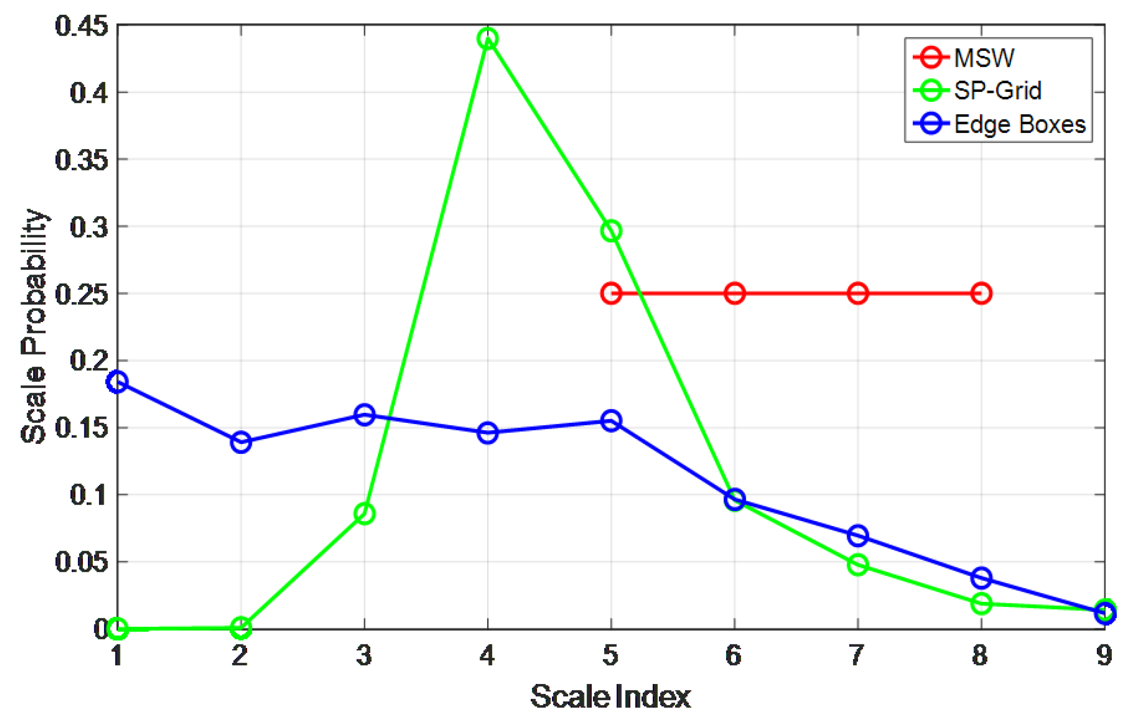
Figure 4 shows the precision–recall curves of two competing methods (Edge-Boxed and SP-Grid) and our MSW approach on the four datasets, and Figure 5 shows the scale distributions of landmarks generated by three methods on all the datasets. In all four datasets, our method significantly outperforms the competing methods and this superior performance is consistent regardless of whether the appearance changes between repeating visits are due to viewpoint (Figure 4a,b) or illumination (Figure 4c,d).
We attribute this improvement in performance to the difference in the distribution of the landmark scale (size), as depicted in Figure 5. Edge Boxes tends to produce a high number of small landmarks and the scale distribution is non-uniform. SP-Grid produces a peaked landmark scale distribution at close to scale index 4. As discussed below, a large number of small landmarks contributes negatively toward matching accuracy of Edge Boxes, and a peaked distribution with SP-Grid reduces its ability to handle viewpoint changes when matching landmarks have different scales.
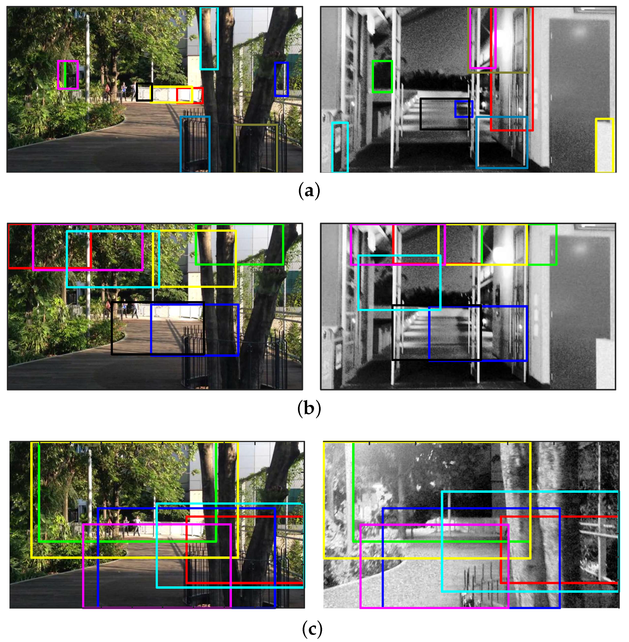
Figure 6 provides qualitative results of the three competing methods in matching one pair of images from the Gardens Point Campus dataset, with Edge Boxes (Figure 6a), SP-Grid (Figure 6b) and our MSW method (Figure 6c), where bounding boxes (landmarks) of the same color are considered to be matching. Both Edge Boxes and SP-Grid produced a false positive result, whereas our method produced a correct true positive result. The failure of Edge Boxes is caused by the small objects, whereas that of SP-Grid is caused by the peaked distribution of landmark (bounding box) scale.
Finally, we compared the proposed method with the state-of-the-arts using average precision (AP). As presented in Table 2, our method quantitatively beats Edge Boxes and SP-Grid method, and this result is consistent with those provided above. Besides, the proposed method significantly outperforms the NetVLAD, a deep model based approach using more compact representation on Gardens Point Campus dataset, and our MSW method achieves comparable performance on the other three datasets. This demonstrates the effectiveness of our method.

4.3. Detailed Analysis of Landmark Scale and Space Distributions

We first verified through a controlled experiment our assertion that scale distribution of the landmarks is important to the performance of landmark-based place recognition in recognizing scenes with significant viewpoint changes. Figure 7a shows three representative scale distributions used in the experiment where Set 1 is the uniform distribution we used in our proposed method, and Sets 2 and 3 are non-uniform distributions where either small landmarks (Set 2) or large landmarks (Set 3) dominate. The recall–precision curves in Figure 7b,c, obtained from the Mapillary Berlin and Gardens Point Campus datasets, support our conclusion that a uniform distribution of landmark scale provides the optimal result. In contrast, when there is little viewpoint change, as in the Freiburg Across Seasons dataset, recognition performance is independent of the landmark scale distribution (Figure 7d). Qualitative results of the experiment are shown in Figure 8 in which our proposed MSW method is able to handle scenes with both significant and minor viewpoint change (Figure 8a,b, respectively), correctly matching landmarks at different scales and the same scale, respectively.
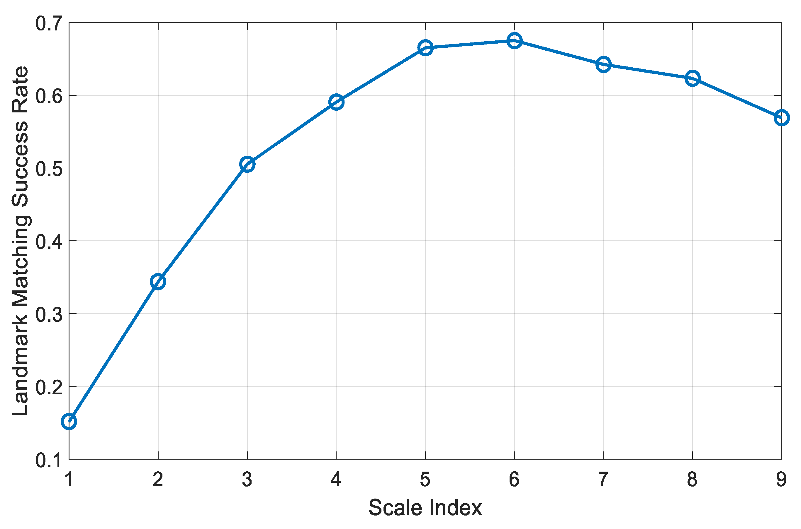
Another important assumption of our MSW method is that landmarks at small scales are not as reliable as those at the higher scales. This assumption is verified by the result shown in Figure 9 that plots landmark matching success rate with respect to landmark scale, using sample images in the Gardens Point Campus dataset whose ground truth for matching landmarks was produced manually. Clearly, small landmarks are not as reliable as landmarks at higher scales. This contributes to the poor performance of landmarks generation methods whose landmark population is dominated by small landmarks such as Edge Boxes.
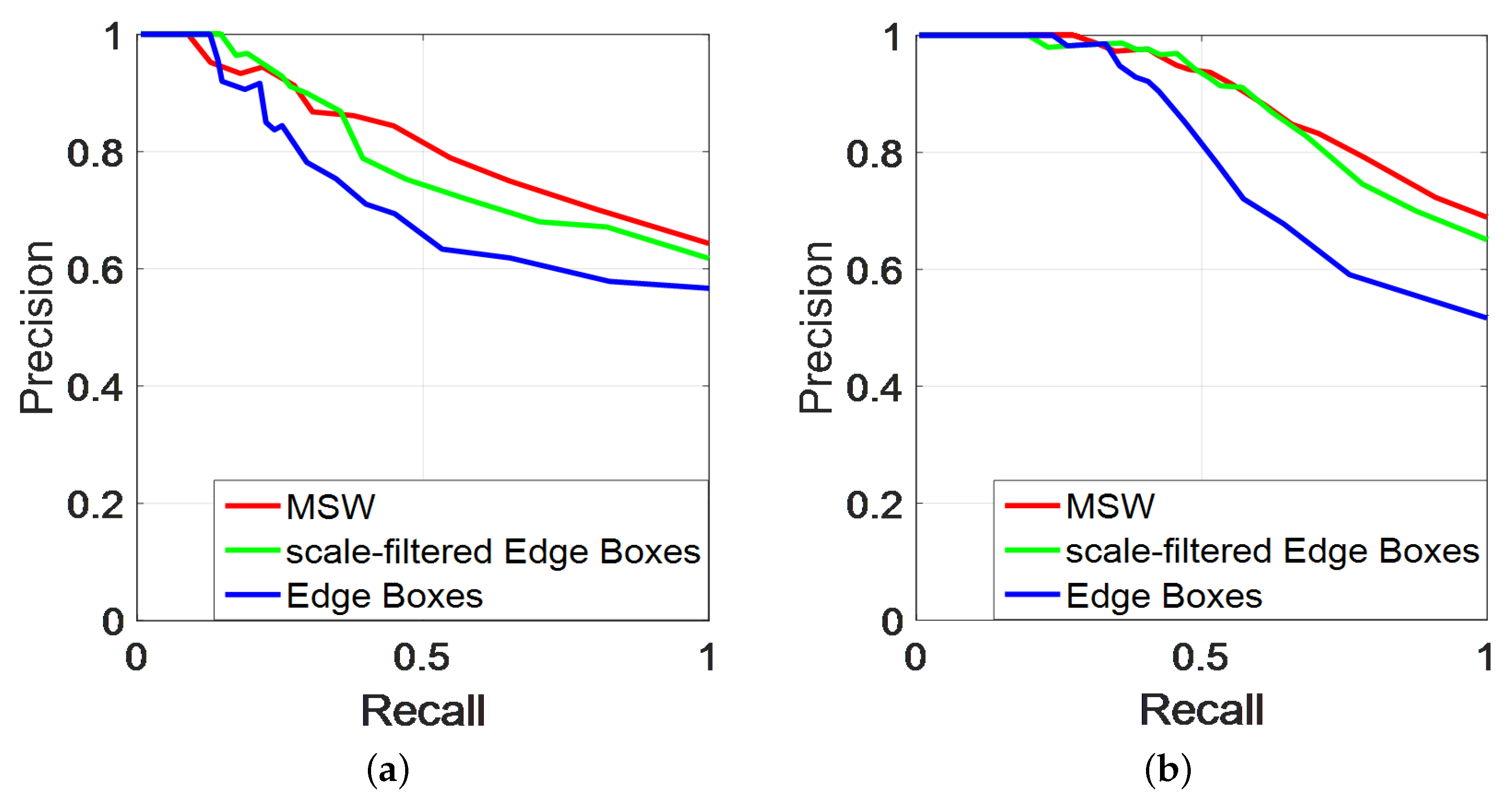
Furthermore, to analyze the impact of the small-scale landmarks on the recognition performance, from the candidate regions generated by Edge Boxes, we removed the landmarks with scales smaller than 0.1 and used the remaining 100 regions for feature matching. We then compared the performance of the method that uses the original Edge Boxes landmarks vs. scale-filtered Edge Boxes landmarks on Mapillary Berlin and Freiburg Across Seasons datasets. As shown in Figure 10, the performance of the scale-filtered Edge Boxes using only landmarks at large scales is slightly worse than our MSW method, whereas it is significantly better than the original Edge Boxes on both datasets. This indicates that landmarks at higher scales tend to improve performance.
In addition, landmarks at scales approaching 1.0 are similar to using the whole image with poor shift-invariance property [13,34], and their use should therefore be discouraged as well.
Finally, we include an observation on the spatial landmark distributions of the three competing methods. While our MSW and SP-Grid produce uniform spatial distribution of the landmarks for both query and reference images, as illustrated in Figure 11b,c, methods using object proposals as the basis for landmark generation such as Edge Boxes often produce uneven spatial distribution (Figure 11d). Intuitively, in Figure 11d, landmarks in query image are distributed in the left side, whereas their counterparts in reference image account for the right side of the image, which makes the matching difficult and, thus, results in the false matches. In addition, it is observed that much of an image with rich texture contents is not involved in the recognition process, and this could be detrimental to the recognition performance.
Although it is generally effective, our method still inevitably produces biased matching results in some cases. Analysis of the experimental results shows that, during object detection and matching, our MSW method commit mistakes due to the following specific reasons:
On the one hand, in its attempt to involve the entire image in matching, MSW includes texture-poor regions (e.g., sky and road), which can contribute to false positive landmark matches due to their similarity. Edge Boxes can in general avoid these false positives better than MSW, however, at the expense of not involving the entire image. Overall, the benefit of involving the entire image outweighs the cost of false positive mistakes, as we have shown in our experiments of comparing MSW with Edge Boxes.
On the other hand, although CNN-based features show increased discriminating power with respect to traditional hand-crafted features, they are far from being perfect and, as a result, inevitably cause false matches (both false positive and false negative). This can be easily seen in all our experiments where the precision–recall curves have much to improve, especially on the challenging datasets, and further improvement of landmark descriptors is definitely an open area of research.
Our future work will focus on alleviating the above-mentioned drawbacks and further improving the performance of our MSW method. Besides, we will improve the efficiency of our method through introducing the BoCNF [15], which is an efficient image matching method with Bag of ConvNet features to our system.

5. Conclusions

In this paper, we propose a novel method for generating landmarks for landmark-based visual place recognition systems. Our method is based on the observations that, since existing methods for generating landmarks are based on object detection, they lead to landmarks: (a) whose sizes are skewed toward the small scales or uneven with respect to scale; and (b) whose spatial distribution poorly covers an image. Small landmarks are not as discriminating as larger landmarks, and uneven distribution of landmark scale is not conducive for handling viewpoint changes such as zooming. Our proposed method in contrast uses a MSW procedure to guarantee a uniform distribution of landmark scale as well as landmark spatial coverage. We demonstrated the clear advantage of our proposed landmark generation method experimentally on several popular datasets that involve significant viewpoint and illumination changes, over representative object-based methods for landmark generation. Due to these characteristics of our proposed method, it can significantly improve the recognition accuracy compared with the state-of-the art approaches. In addition, our method provides a finer landmark generation approach and has the advantage of being computationally efficient as it uses a sliding window process with a single parameter (the scales of landmarks desired) that does not require any image processing operations.

Author Contributions

Conceptualization, B.Y., H.Z. and X.X.; methodology, B.Y.; software, B.Y.; validation, B.Y. and J.L.; formal analysis, B.Y.; writing—original draft preparation, B.Y.; writing—review and editing, H.Z.; supervision, H.Z.; and funding acquisition, X.X.

Funding

This research was funded by the National Natural Science Foundation of China (Grant Nos. 61473085, 51775110, and 61703096) and the Natural Science Foundation of Jiangsu Province (No. BK20170691).

Acknowledgments

This work was completed during Bo Yang’s visit to the Department of Computing Science at University of Alberta.

Conflicts of Interest

The authors declare no conflict of interest.

References

  1. Chen, Z.; Liu, L.; Sa, I.; Ge, Z.; Chli, M. Learning Context Flexible Attention Model for Long-Term Visual Place Recognition. IEEE Robot. Autom. Lett. 2018, 3, 4015–4022. [Google Scholar] [CrossRef] [Green Version]
  2. Johns, E.; Yang, G.Z. Generative Methods for Long-Term Place Recognition in Dynamic Scenes. Int. J. Comput. Vis. 2014, 106, 297–314. [Google Scholar] [CrossRef]
  3. Naseer, T.; Burgard, W.; Stachniss, C. Robust Visual Localization Across Seasons. IEEE Trans. Robot. 2018, 34, 289–302. [Google Scholar] [CrossRef]
  4. Lowry, S.; Sünderhauf, N.; Newman, P.; Leonard, J.J.; Cox, D.; Corke, P.; Milford, M.J. Visual Place Recognition: A Survey. IEEE Trans. Robot. 2016, 32, 1–19. [Google Scholar] [CrossRef]
  5. Milford, M.J.; Wyeth, G.F. SeqSLAM: Visual route-based navigation for sunny summer days and stormy winter nights. In Proceedings of the 2012 IEEE International Conference on Robotics and Automation, Saint Paul, MN, USA, 14–18 May 2012; pp. 1643–1649. [Google Scholar]
  6. Neubert, P.; Sünderhauf, N.; Protzel, P. Appearance change prediction for long-term navigation across seasons. In Proceedings of the 2013 European Conference on Mobile Robots, Barcelona, Spain, 25–27 September 2013; pp. 198–203. [Google Scholar]
  7. McManus, C.; Churchill, W.; Maddern, W.; Stewart, A.D.; Newman, P. Shady dealings: Robust, long-term visual localisation using illumination invariance. In Proceedings of the 2014 IEEE International Conference on Robotics and Automation (ICRA), Hong Kong, China, 31 May–7 June 2014; pp. 901–906. [Google Scholar]
  8. Caduff, D.; Timpf, S. On the assessment of landmark salience for human navigation. Cogn. Process. 2008, 9, 249–267. [Google Scholar] [CrossRef] [PubMed]
  9. Keil, J.; Edler, D.; Dickmann, F.; Kuchinke, L. Meaningfulness of landmark pictograms reduces visual salience and recognition performance. Appl. Ergon. 2019, 75, 214–220. [Google Scholar] [CrossRef] [PubMed]
  10. Zhang, H. BoRF: Loop-closure detection with scale invariant visual features. In Proceedings of the IEEE International Conference on Robotics and Automation (ICRA), Shanghai, China, 9–13 May 2011; pp. 3125–3130. [Google Scholar]
  11. Cummins, M.; Newman, P. FAB-MAP: Probabilistic Localization and Mapping in the Space of Appearance. Int. J. Robot. Res. 2008, 27, 647–665. [Google Scholar] [CrossRef]
  12. Sünderhauf, N.; Shirazi, S.; Jacobson, A.; Dayoub, F.; Pepperell, E.; Upcroft, B.; Milford, M. Place recognition with ConvNet landmarks: Viewpoint-robust, condition-robust, training-free. In Proceedings of the Robotics: Science and Systems, Rome, Italy, 13–17 July 2015. [Google Scholar]
  13. Sünderhauf, N.; Shirazi, S.; Dayoub, F.; Upcroft, B.; Milford, M. On the performance of ConvNet features for place recognition. In Proceedings of the 2015 IEEE/RSJ International Conference on Intelligent Robots and Systems (IROS), Hamburg, Germany, 28 September–2 October 2015; pp. 4297–4304. [Google Scholar]
  14. Neubert, P.; Protzel, P. Local region detector + CNN based landmarks for practical place recognition in changing environments. In Proceedings of the 2015 European Conference on Mobile Robots (ECMR), Lincoln, UK, 2–4 September 2015; pp. 1–6. [Google Scholar]
  15. Hou, Y.; Zhang, H.; Zhou, S. BoCNF: efficient image matching with Bag of ConvNet features for scalable and robust visual place recognition. Auton. Robot. 2018, 42, 1169–1185. [Google Scholar] [CrossRef]
  16. Jégou, H.; Douze, M.; Schmid, C.; Pérez, P. Aggregating local descriptors into a compact image representation. In Proceedings of the IEEE Conference on Computer Vision and Pattern Recognition (CVPR), San Francisco, CA, USA, 13–18 June 2010; pp. 3304–3311. [Google Scholar]
  17. Zitnick, C.L.; Dollár, P. Edge Boxes: Locating Object Proposals from Edges. In Proceedings of the European Conference on Computer Vision (ECCV), Zurich, Switzerland, 6–12 September 2014; pp. 391–405. [Google Scholar]
  18. Ren, S.; He, K.; Girshick, R.; Sun, J. Faster R-CNN: Towards Real-Time Object Detection with Region Proposal Networks. IEEE Trans. Pattern Anal. Mach. Intell. 2017, 39, 1137–1149. [Google Scholar] [CrossRef] [PubMed] [Green Version]
  19. Simonyan, K.; Zisserman, A. Very deep convolutional networks for large-scale image recognition. In Proceedings of the International Conference on Learning Representations (ICLR), Banff, AB, Canada, 14–16 April 2014; pp. 1–14. [Google Scholar]
  20. Krizhevsky, A.; Sutskever, I.; Hinton, G.E. ImageNet Classification with Deep Convolutional Neural Networks. In Advances in Neural Information Processing Systems 25; NIPS: Cambridge, MA, USA, 2012; pp. 1097–1105. [Google Scholar]
  21. He, K.; Zhang, X.; Ren, S.; Sun, J. Deep Residual Learning for Image Recognition. In Proceedings of the IEEE Conference on Computer Vision and Pattern Recognition (CVPR), Las Vegas, NV, USA, 27–30 June 2016; pp. 770–778. [Google Scholar]
  22. Cheng, M.; Zhang, Z.; Lin, W.; Torr, P. BING: Binarized Normed Gradients for Objectness Estimation at 300fps. In Proceedings of the IEEE Conference on Computer Vision and Pattern Recognition (CVPR), Columbus, OH, USA, 24–27 June 2014; pp. 3286–3293. [Google Scholar]
  23. Lowe, D.G. Object recognition from local scale-invariant features. In Proceedings of the IEEE International Conference on Computer Vision (ICCV), Corfu, Greece, 21–22 September 1999; pp. 1150–1157. [Google Scholar]
  24. Oliva, A.; Torralba, A. Modeling the Shape of the Scene: A Holistic Representation of the Spatial Envelope. Int. J. Comput. Vis. 2001, 42, 145–175. [Google Scholar] [CrossRef]
  25. Chen, Z.; Lam, O.; Jacobson, A.; Milford, M. Convolutional Neural Network-based Place Recognition. arXiv 2014, arXiv:1411.1509. [Google Scholar]
  26. Naseer, T.; Spinello, L.; Burgard, W.; Stachniss, C. Robust Visual Robot Localization Across Seasons Using Network Flows. In Proceedings of the Twenty-Eighth AAAI Conference on Artificial Intelligence, Quebec City, QC, Canada, 27–31 July 2014; pp. 2564–2570. [Google Scholar]
  27. Cascianelli, S.; Costante, G.; Bellocchio, E.; Valigi, P.; Fravolini, M.L.; Ciarfuglia, T.A. Robust visual semi-semantic loop closure detection by a covisibility graph and CNN features. Robot. Auton. Syst. 2017, 92, 53–65. [Google Scholar] [CrossRef]
  28. Hou, Y.; Zhang, H.; Zhou, S. Evaluation of Object Proposals and ConvNet Features for Landmark-based Visual Place Recognition. J. Intell. Robot. Syst. 2018, 92, 505–520. [Google Scholar] [CrossRef]
  29. Hosang, J.; Benenson, R.; Dollár, P.; Schiele, B. What Makes for Effective Detection Proposals? IEEE Trans. Pattern Anal. Mach. Intell. 2016, 38, 814–830. [Google Scholar] [CrossRef] [PubMed]
  30. Redmon, J.; Farhadi, A. YOLO9000: Better, Faster, Stronger. In Proceedings of the IEEE Conference on Computer Vision and Pattern Recognition (CVPR), Honolulu, HI, USA, 21–26 July 2017; pp. 6517–6525. [Google Scholar]
  31. Arbeláez, P.; Pont-Tuset, J.; Barron, J.; Marques, F.; Malik, J. Multiscale Combinatorial Grouping. In Proceedings of the IEEE Conference on Computer Vision and Pattern Recognition (CVPR), Columbus, OH, USA, 24–27 June 2014; pp. 328–335. [Google Scholar]
  32. Uijlings, J.R.R.; van de Sande, K.E.A.; Gevers, T.; Smeulders, A.W.M. Selective Search for Object Recognition. Int. J. Comput. Vis. 2013, 104, 154–171. [Google Scholar] [CrossRef] [Green Version]
  33. Krähenbühl, P.; Koltun, V. Learning to propose objects. In Proceedings of the IEEE Conference on Computer Vision and Pattern Recognition (CVPR), Las Vegas, NV, USA, 26 June–1 July 2015; pp. 1574–1582. [Google Scholar]
  34. Neubert, P.; Protzel, P. Beyond Holistic Descriptors, Keypoints, and Fixed Patches: Multiscale Superpixel Grids for Place Recognition in Changing Environments. IEEE Robot. Autom. Lett. 2016, 1, 484–491. [Google Scholar] [CrossRef]
  35. Bingham, E.; Mannila, H. Random Projection in Dimensionality Reduction: Applications to Image and Text Data. In Proceedings of the ACM SIGKDD International Conference on Knowledge Discovery and Data Mining (KDD), San Francisco, CA, USA, 26–29 August 2001; pp. 245–250. [Google Scholar]
  36. Arandjelović, R.; Gronat, P.; Torii, A.; Pajdla, T.; Sivic, J. NetVLAD: CNN Architecture for Weakly Supervised Place Recognition. IEEE Trans. Pattern Anal. Mach. Intell. 2018, 40, 1437–1451. [Google Scholar] [CrossRef]
  37. Maddern, W.; Pascoe, G.; Linegar, C.; Newman, P. 1 Year, 1000km: The Oxford RobotCar Dataset. Int. J. Robot. Res. 2017, 36, 3–15. [Google Scholar] [CrossRef]
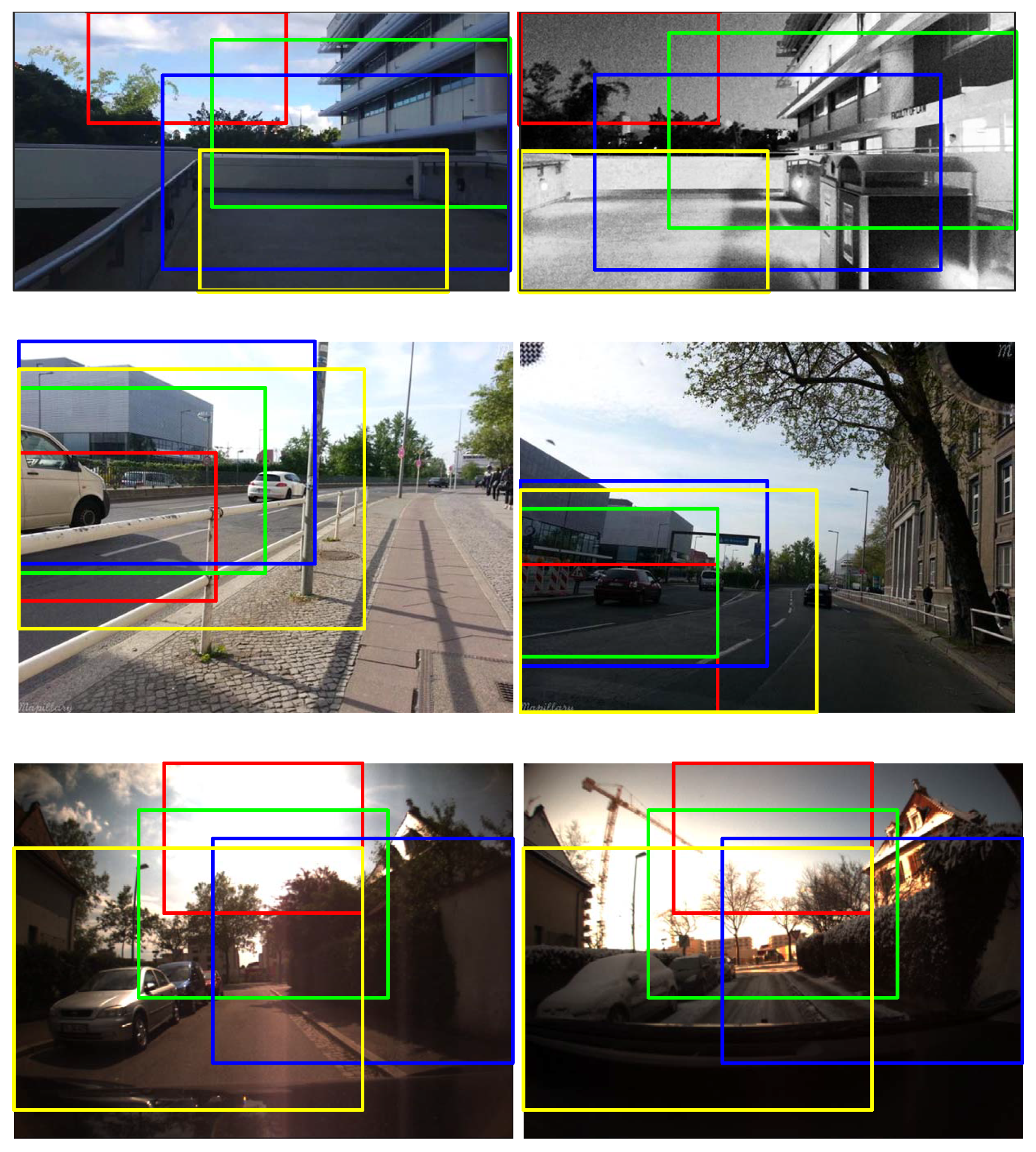
Figure 1. Three examples of the pairwise matching using our approach. Each row presents two correctly matching images while the boxes outlined with the same color in two images denote the successfully matched landmarks. It shows that the landmarks generated using our method is robust to dramatic illumination, viewpoint and seasonal changes (from top to bottom).
Applsci 09 03146 g001
Figure 2. Overview of our MSW based visual place recognition method. First, 100 landmarks are extracted from different scales by MSW strategy. Next, 1024-dimensional CNN features are computed for representing the landmarks before the bi-directional nearest neighbor search conducted to match pairwise landmarks. Thus, the best pairwise match is obtained by pooling all the pairwise matching results for similarity measure.
Applsci 09 03146 g002
Figure 3. An example of extracting 100 landmarks from four scales by MSW. The left image shows the original image. The top right four images illustrate the uniform sampling process with 0.16, 0.25, 0.36 and 0.49 scales, respectively. Twenty-five landmarks are extracted from each scale in this case. The bottom right four images show the examples of landmarks extracted by MSW with four different scales.
Applsci 09 03146 g003
Figure 4. Performance of MSW, SP-Grid and Edge Boxes on: (a) Mapillary Berlin; (b) Gardens Point Campus; (c) Freiburg Across Seasons; and (d) Oxford RobotCar dataset.
Applsci 09 03146 g004
Figure 5. Landmark distribution of MSW, SP-Grid and Edge Boxes on all four datasets. Edge Boxes tends to produce a high number of small landmarks and the scale distribution is non-uniform. SP-Grid produces a peaked landmark scale distribution at close to scale index 4. Scale distribution of our MSW method is uniform.
Applsci 09 03146 g005
Figure 6. An example illustrating the pairwise matching results achieved by: (a) Edge Boxes; (b); SP-Grid; and (c) our MSW method. Both Edge Boxes and SP-Grid produced a false positive result, whereas our method produced a correct true positive result. It is shown that the failure of Edge Boxes is caused by the small objects, whereas that of SP-Grid is caused by the peaked distribution of landmark scale. Our method leads to true positive matches by utilizing the landmarks of appropriate distribution and scales.
Applsci 09 03146 g006
Figure 7. (a) Three representative scale distributions of landmarks. Set 1 shows uniform distributions, while Set 2 and 3 are non-uniform. Results of three settings on: (b) Mapillary Berlin; (c) Gardens Point Campus dataset including large viewpoint changes; and (d) Freiburg Across Seasons dataset with slight viewpoint changes.
Applsci 09 03146 g007
Figure 8. Examples of matched images with extracted and matched landmarks by our MSW method from: (a) Mapillary Berlin dataset; and (b) Freiburg Across Seasons dataset. The matched landmarks on Mapillary Berlin dataset are from different scales, while they have same scales on Freiburg Across Seasons dataset.
Applsci 09 03146 g008
Figure 9. Landmark matching success rate with respect to landmark scales based on bi-directional nearest neighbor search between the “day-left” and “night-right” sequences.
Applsci 09 03146 g009
Figure 10. Results of MSW, scale-filtered Edge Boxes and original Edge Boxes for place recognition on: (a) Mapillary Berlin; and (b) Freiburg Across Seasons dataset
Applsci 09 03146 g010
Figure 11. An example illustrating two images captured at the same place and the corresponding landmark distributions generated using different methods. (a) The query (left) and reference (right) images. The spatial distribution of landmarks extracted from the two images are obtained by: (b) our MSW method; (c) SP-Grid; and (d) Edge Boxes. Deeper color area indicates more coverage by landmarks.
Applsci 09 03146 g011
Table 1. Nine indices with the corresponding scale range.
IndexScale Range
1[0, 0.02)
2[0.02, 0.05)
3[0.05, 0.09)
4[0.09, 0.14)
5[0.14, 0.23)
6[0.23, 0.34)
7[0.34, 0.48)
8[0.48, 0.70)
9[0.70, 1]
Table 2. Comparison of our method with the state-of-the-arts (AP).
NetVLAD [36]SP-Grid [34]Edge Boxes [17]MSW(Our)
Mapillary Berlin0.84410.72420.72850.8231
Gardens Point Campus0.77880.76700.82740.9203
Freiburg Across Seasons0.87480.83590.81090.9040
Oxford RobotCar0.91930.80430.83150.9074