Model-Free Method for Damage Localization of Grid Structure

Abstract

A model-free damage identification method for grid structures based on displacement difference is proposed. The inherent relationship between the displacement difference and the position of structural damage was deduced in detail by the Sherman–Morrison–Woodbury formula, and the basic principle of damage localization of the grid structure was obtained. That is, except for the tensile and compressive deformations of the damaged elements, the deformations of other elements were small, and only rigid body displacements occurred before and after the structural damage. According to this rule, a method for identifying the position of the damage was proposed for the space grid structure by using the rate of change of length for each element. Taking a space grid structure with a large number of elements as an example, the elastic modulus reduction method was used to simulate the damage to the elements, and the static and dynamic test parameters were simulated respectively to obtain the difference in displacement before and after the structural damage. The rate of change of length of each element was calculated based on the obtained displacement difference, and data noise was added to the simulation. The results indicated that the element with the larger length change rate in the structure was the most likely to be damaged, and the damaged element can be accurately evaluated even in the presence of noise in data.

1. Introduction

In construction, buildings with large spans are becoming increasingly common, and lightweight, economical, beautiful grid structures have become the first choice for roofs. While these grid structures remain in service, damage will accumulate with the long-term effects of loads, material aging, fatigue, accidental loads, and environmental corrosion. If the damaged elements in the structure cannot be identified in time, serious accidents may result. In recent decades, many scholars have comprehensively studied [1,2,3] the damage identification of large structures. For example, Yin et al. [4] studied the degree of element damage in the quadrangular pyramid structure by simulating the displacement-time curve of the unit node, indicating that the displacement relationship can reflect the damage to the grid structure. Wang et al. [5] can accurately determine the damage positions of grid element units using hammer strokes to obtain the structural time domain signals. Li [6] combined the static virtual deformation method and the sequence quadratic programming algorithm for damage identification to quickly and accurately identify damage positions. Ouyang et al. [7] identified damage by the cubic interpolation of bending deflection of the beam in the case of smaller stress redistributions, after assuming structural damages. Huang et al. [8,9] used a random damage index to quantify the damage of a random beam structure through the static test, while considering the model and measurement errors. Hosseinzadeh et al. [10] recognized damage identification as the process of optimizing the stiffness to match the external force with the displacement and proposed a method for calculating the static displacement using flexibility, as well the cuckoo and optimization algorithm to identify damages. The displacement influence line [11] and strain influence line [12] are also used to identify the damage, and Alexandre Kawano conjectured that the time to measure the structural displacement also affects the result [13]. Most of the above studies are based on the model correction technique, which is a common method for damage identification [14,15,16], using finite element models. Nevertheless, it is difficult to establish accurate finite element models for large structures. In order to avoid finite element modeling, Yang et al. [17] used the Sherman–Morrison–Woodbury (SMW) formula to discuss the theoretical basis of structural damage localization in detail. Additionally, they took a beam structure and rigid frame structure as examples to explain the application of this theoretical basis to achieve damage localization. However, the grid structure has not been specifically discussed.

In view of this, the principle in literature [17] was applied to the grid structure to deduce the physical connection between the position of damage and variation in displacement of the grid structure in detail. It was concluded that the basic principle of damage localization of the grid structure before and after the structural damage were small and only the rigid body displacement occurred, except for tensile and compressive deformations of damaged elements. Based on this, the rate of length change of each element was used as the index to identify the damage position for the space grid structure. The proposed method can realize damage recognition without a model, thus avoiding the complicated finite element modeling process, and can be implemented by using static or dynamic test data. Taking the space grid structure with 71 elements as an example, the static and dynamic test parameters were simulated respectively. The length change rate of the element was calculated according to the obtained displacement difference. At the same time, data noise was added to the simulation. The simulation results indicated that the element with the larger rate of length change is the most likely to appear damaged, and the damaged element can be accurately evaluated even if the data are noisy.

2. Basic Principle of Structural Damage Localization Based on Displacement Difference

There are many displacement-based damage identification methods [18,19,20], but none of them can explain the physical connection between the position of damage and the displacement. Generally, considering a structure with $n$ degrees of freedom, the displacement under the action of static loads should satisfy the following equation:

$$Ku=l$$

(1)

where K(n × n) is the overall stiffness matrix of the undamaged structure and u is the displacement vector under the static load vector l. Equation (1) can be expressed as:

$$u=Fl$$

(2)

where F is the flexibility matrix of the undamaged structure, that is, F = K⁻¹. Structural damage can result in a decrease in the stiffness and increase in flexibility. The model matrix of the undamaged structure is related to the model matrix of the damaged structure as follows:

$$F_d=F+\Delta F$$

(3)

$$K_d=K-\Delta K$$

(4)

The displacement u_d produced after structural damage can be expressed as:

$$u_d=F_{d}l$$

(5)

Therefore, the displacement change ∆u can be expressed as:

$$\Delta u=u_d-u=\Delta Fl=[{(K-\Delta K)}^{-1}-K^{-1}]$$

(6)

In order to further develop Equation (6), the following SMW formula is used:

$${(K+X{Y}^T)}^{-1}=K^{-1}-K^{-1}X{(I+Y^T{K}^{-1}X)}^{-1}{Y}^T{K}^{-1}$$

(7)

∆K = ∆KI^T, using Equation (7) to simplify Equation (6) can obtain Equation (8):

$$\Delta u=K^{-1}\Delta K{(I-K^{-1}\Delta K)}^{-1}{K}^{-1}l$$

(8)

In order to express the relationship between the change in displacement and damages, Equation (8) can be rewritten as:

$$\Delta u=\delta d_i$$

(9)

$$d_i=K^{-1}\Delta K$$

(10)

$$\delta ={(I-K^{-1}\Delta K)}^{-1}{K}^{-1}l$$

(11)

The physical meaning of Equation (9) is very important. This equation indicates that displacement change ∆u of the structure before and after damage was a linear combination of characteristic displacements. According to Equation (10), the characteristic displacement di was obtained by applying the non-zero column vector in ∆K as a static load to the structure, and these non-zero column vectors in ∆K can be defined as characteristic forces. The characteristic force and characteristic displacement are different for different structure types. The characteristic forces and displacements of the beam structure and rigid frame structure have been discussed in detail in literature [17]. In the following chapters, we will discuss the characteristic force and displacement of grid structures in detail and obtain the basic principle of the damage localization of the grid structure.

3. Damage Identification of Grid Structure

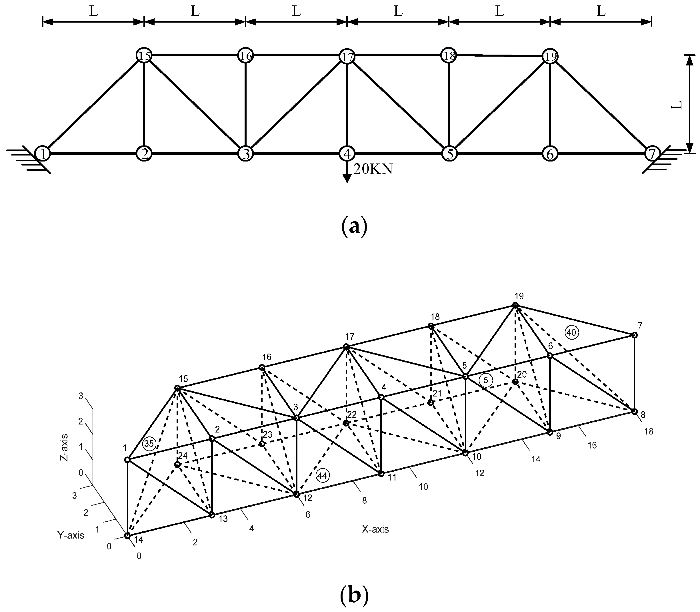
3.1. Characteristic Force and Displacement of Grid Structure

Generally, the structure shown in Figure 1 was taken as an example to illustrate the characteristic force and displacement of the grid structure, and the essential relationship between the displacement difference and the damage position was analyzed. The node displacement vector in the structure and the element stiffness matrix in the local coordinate system are expressed as:

$$u^e={[x_1\hspace{1em}{y}_1\hspace{1em}{x}_2\hspace{1em}{y}_2]}^T$$

(12)

$$K_i^e=\frac{EA}{L}\left[\begin{array}{cccc}1& 0& -1& 0\\ 0& 0& 0& 0\\ -1& 0& 1& 0\\ 0& 0& 0& 0\end{array}\right]$$

(13)

Taking the No. 3 element in Figure 1 as an example, the element stiffness matrix in the global coordinate system of the element and the corresponding ∆K are expressed as:

$$K_i^e=\frac{EA}{L}\left[\begin{array}{cccc}\frac{1}{4}& -\frac{\sqrt{3}}{4}& -\frac{1}{4}& \frac{\sqrt{3}}{4}\\ -\frac{\sqrt{3}}{4}& \frac{3}{4}& \frac{\sqrt{3}}{4}& -\frac{3}{4}\\ -\frac{1}{4}& \frac{\sqrt{3}}{4}& \frac{1}{4}& -\frac{\sqrt{3}}{4}\\ \frac{\sqrt{3}}{4}& -\frac{3}{4}& -\frac{\sqrt{3}}{4}& \frac{3}{4}\end{array}\right]$$

(14)

$$\Delta K={\displaystyle \sum {\alpha }_i{k}_i}$$

(15)

where α_i and K_t are the damage coefficient and element stiffness matrix in the global coordinate system of the ith element, respectively, and E, A, and L are the elastic modulus, section area, and length of element, respectively. The first column of the non-zero vector in ∆K is applied as the characteristic force to the No. 3 element, as shown in Figure 2:

It can be seen from Figure 2 that the element 3 was in a state of force equilibrium. The same result can be obtained by using the remaining non-zero column vectors as characteristic forces. The above results are universal, namely: (1) The characteristic force was the balance force system. (2) The characteristic force of an element affects only that element, without affecting other elements. Therefore, when the characteristic force is applied to the structure, the corresponding characteristic displacement has the following characteristics: only the element corresponding to the characteristic force exhibited tensile and compressive deformations, while the other elements were free from the effect of forces and only performed rigid body motions. Furthermore, the change in structural displacement change due to damages was a linear combination of the characteristic displacements associated with the damaged elements. As for the displacement difference vector under any load, except for tensile or compressive deformations of damaged elements, the other elements only performed rigid body movements, without significant deformations. Therefore, the rate of length change of each element can be calculated according to the displacement difference of the structure before and after the damage, and the element with the larger rate of length change was the position where the damage was most likely to occur.

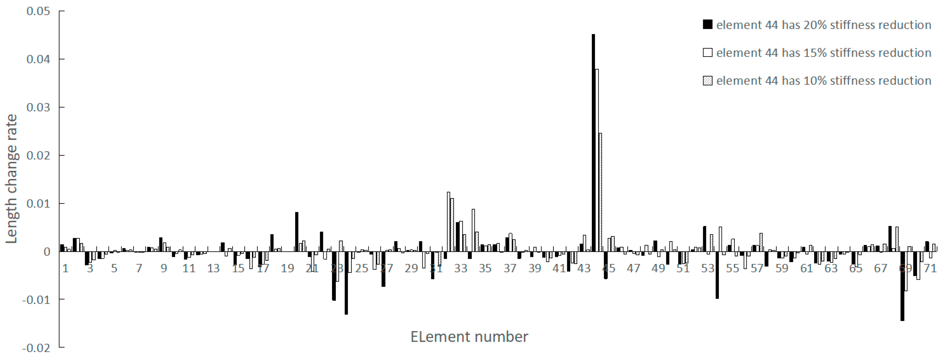
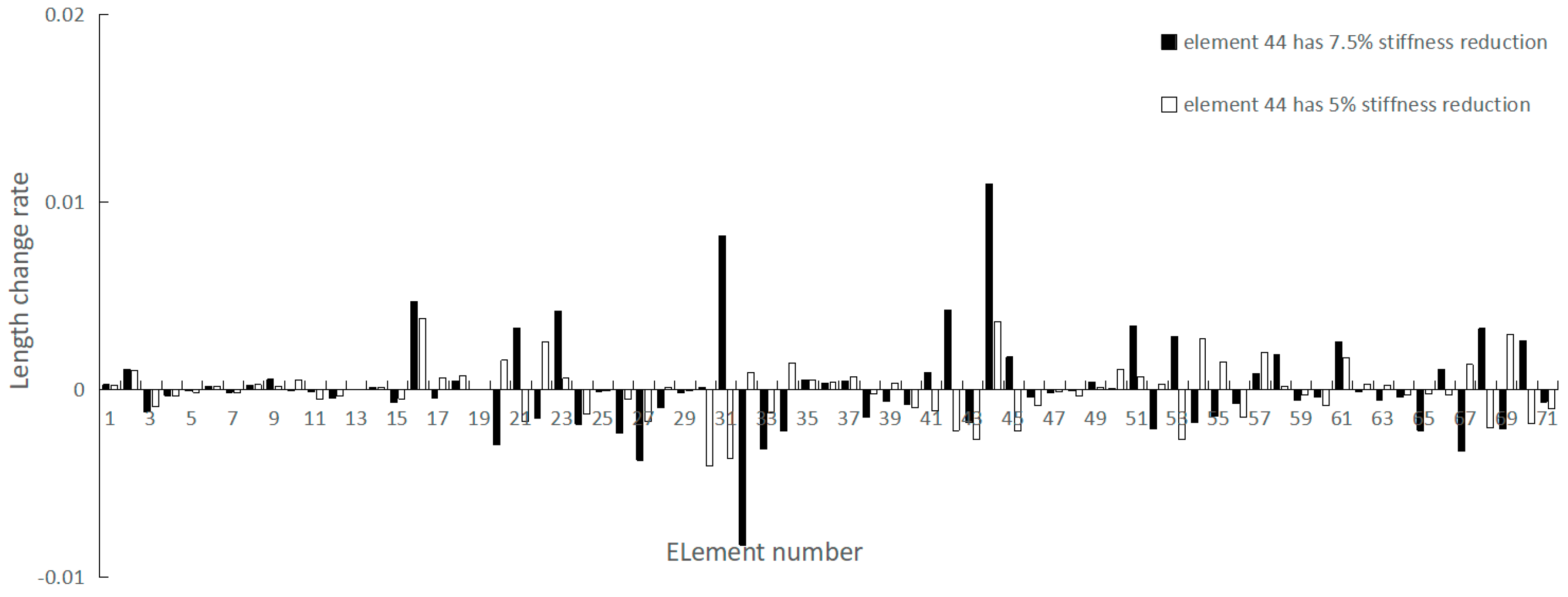
3.2. Damage Localization of Grid Structure Based on Displacement Difference

Measurement of static displacements can be performed by many different methods. Most often used are traditional techniques, using precise leveling, dial gauge, or inductive gauge. Recently, optical systems for displacement measurement have been successfully applied in actual engineering, and good effects were achieved, such as photogrammetry, laser techniques, and visual techniques. More details about displacement measurement can be found in References [21,22,23,24,25].

According to the measured displacement difference before and after the damage of each node, the rate of length change of each element can be calculated. The calculation formula is derived as follows:

The displacement difference can be decomposed as the displacement difference ∆u_x, ∆u_y, and ∆u_z in the x, y, and z direction, respectively. The calculation formula of the length of each element in the damaged structure is expressed as:

$$L_d=\sqrt{{(x_1-x_2)}^2+{(y_1-y_2)}^2+{(z_1-z_2)}^2}$$

(16)

$$x_1=x_0+\Delta u_x,\hspace{0.17em}{y}_1=y_0+\Delta u_y,\hspace{0.17em}{z}_1=x_0+\Delta u_z$$

(17)

where x₀, y₀, and z₀ refer to original coordinates of the previous node of the element in the x, y, and z directions, respectively, x₁, y₁, and z₁ refer to original coordinates plus the coordinates of ∆u_x, ∆u_y, and ∆u_z , respectively, and x₂, y₂, and z₂ refer to original coordinates of the post node of the element plus coordinates of the displacement difference ∆u_x, ∆u_y, and ∆u_z of the corresponding node. Using the results obtained in Equation (16), the change in length of the element before and after damage is expressed as:

$$\Delta L=L_d-L$$

(18)

where L refers to the original length of the structural element. According to Equation (18), the rate of length change of the element is expressed as:

$$\epsilon =\frac{\Delta L}{L}$$

(19)

The determination of the damage position can be made based on the computed change rate of element length.

In summary, the damage localization of grid structure based on the displacement difference has the following steps:

(1)

Obtain the displacement difference ∆u through experiment. It is preferred to use a laser range finder to obtain the displacement difference in the static test. If a static test cannot be performed, we can use the dynamic flexibility method to indirectly obtain the displacement difference (multiply the virtual force vector by the dynamic flexibility difference matrix before and after damage). Similarly, it is not necessary to establish a finite element model when the dynamic flexibility method is used. The approximate flexibility difference matrix can be obtained by the following formula:

$$\Delta F=F_d-F$$

(20)

$$F={\displaystyle \sum _{j=1}^m\frac{1}{{\lambda }_j}}{\phi }_j{\phi }_j^T$$

(21)

where F and F_d are the flexibility matrices before and after damage, respectively, m is the measured number of modes, and λ_j and φ_j are the _jth order eigenvalues and eigenvectors (mode shapes), respectively. The flexibility matrix difference obtained by the dynamic flexibility method was considered in the following equation to obtain the change in displacement:

$$\Delta u=\Delta F\cdot l_v$$

(22)

where l_v is the virtual force vector. Theoretically, the virtual vector can be selected arbitrarily according to need. For example, l_v = [0 --- 1 --- 0]^T. The specific steps for the selection of the virtual force vector can be obtained from literature [1];

(2)

The length of element after damage was calculated by Equation (16), and the change in length of the element before and after damage was calculated by Equation (18).

(3)

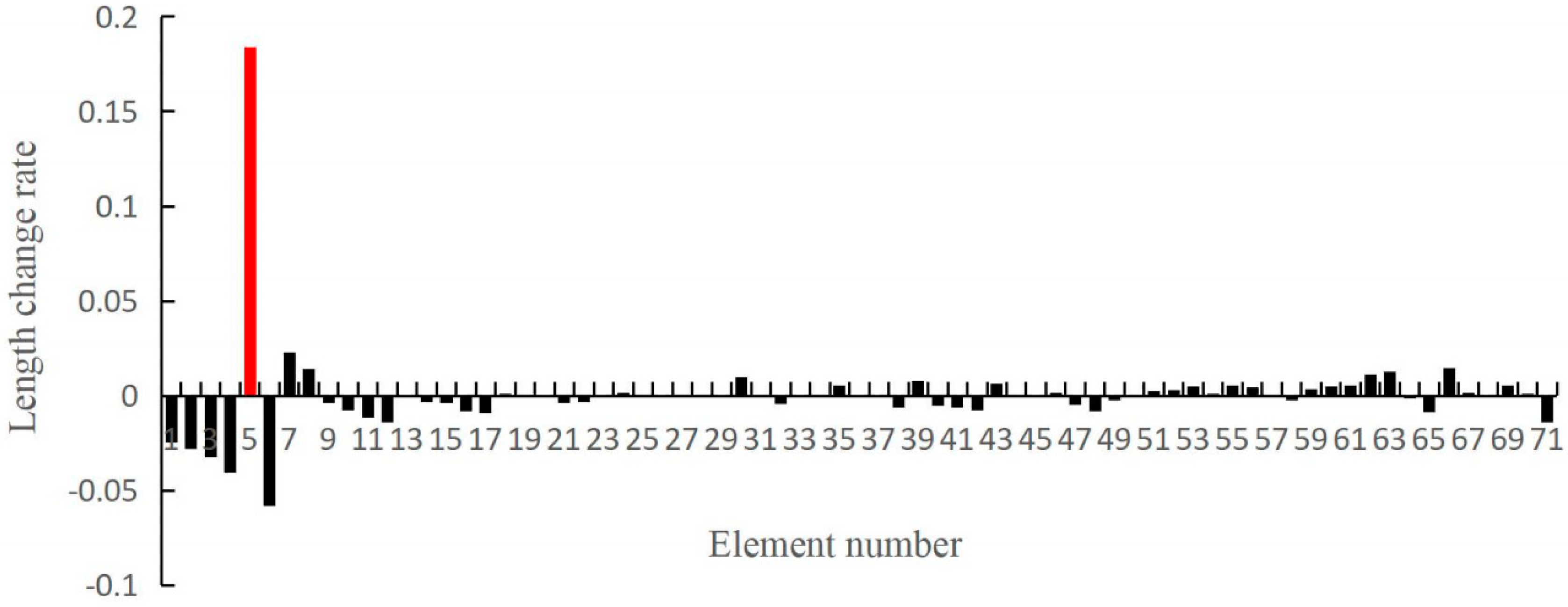
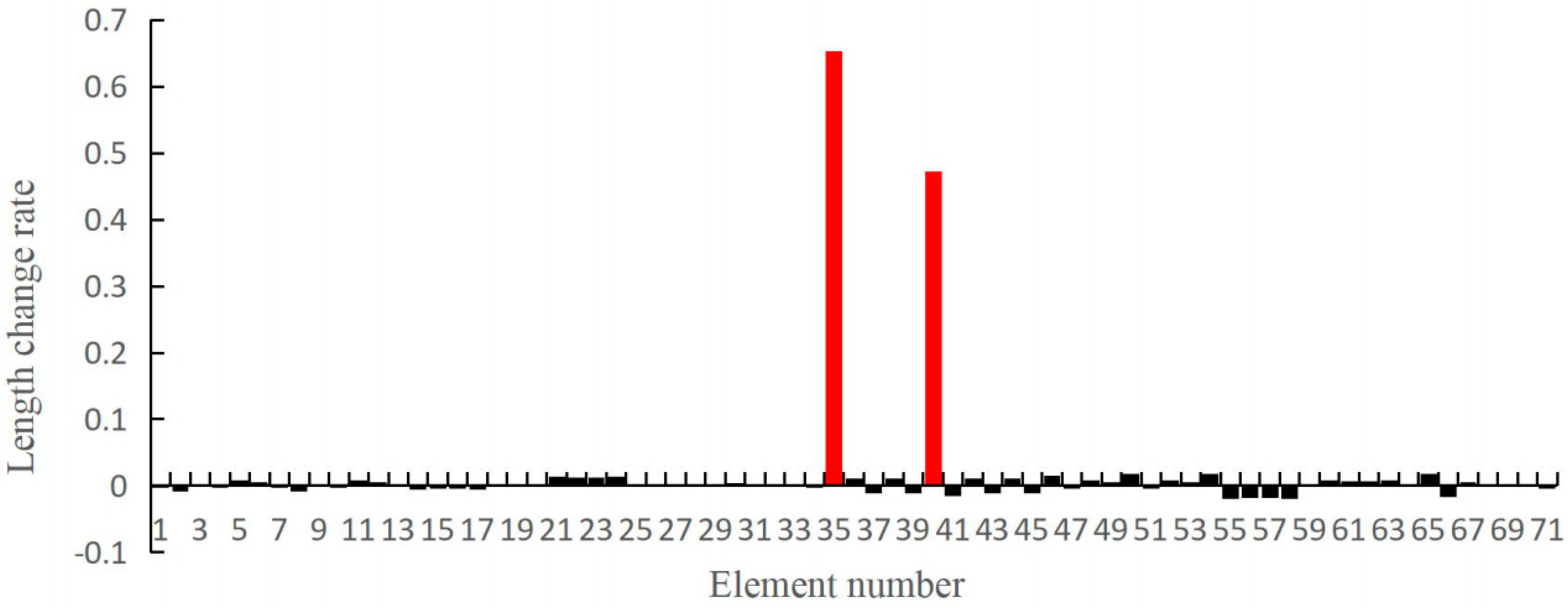
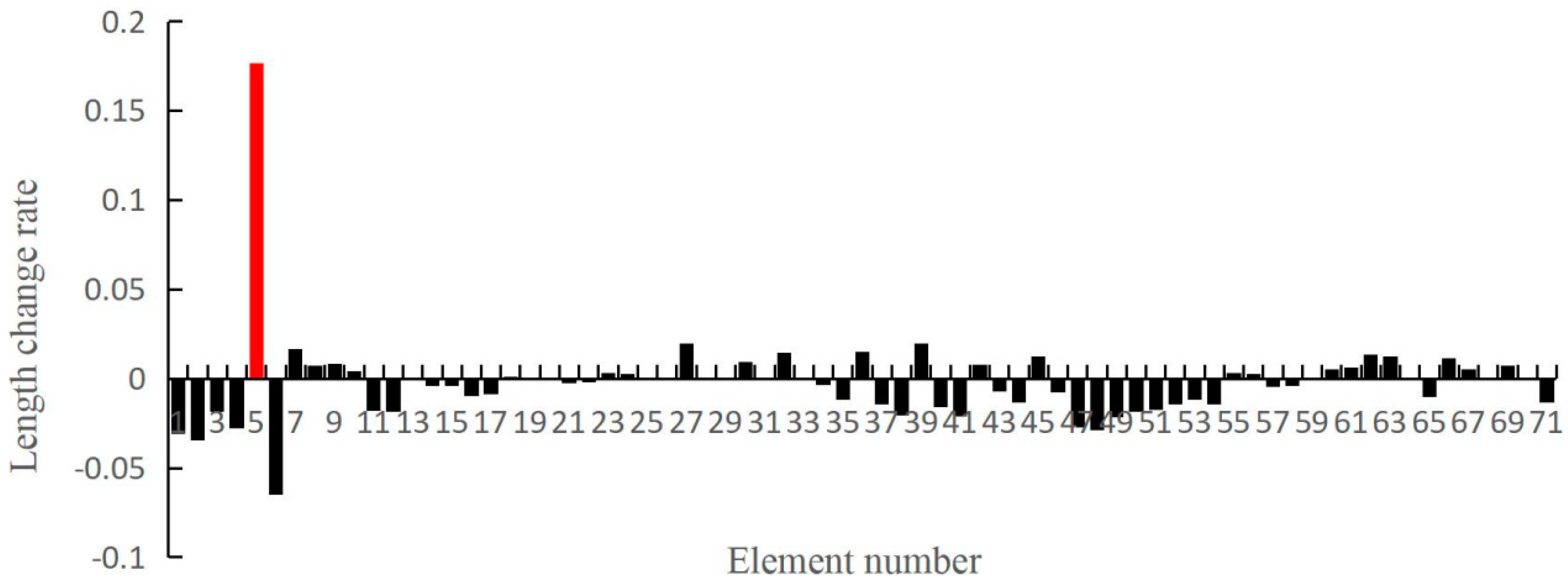
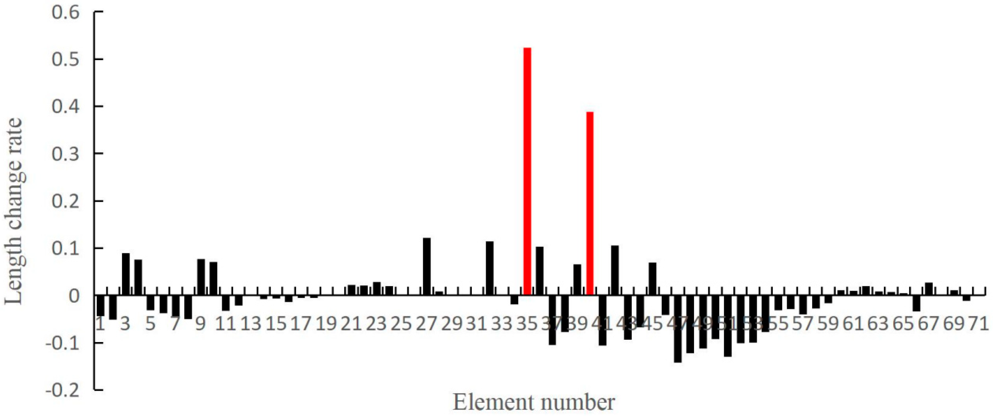
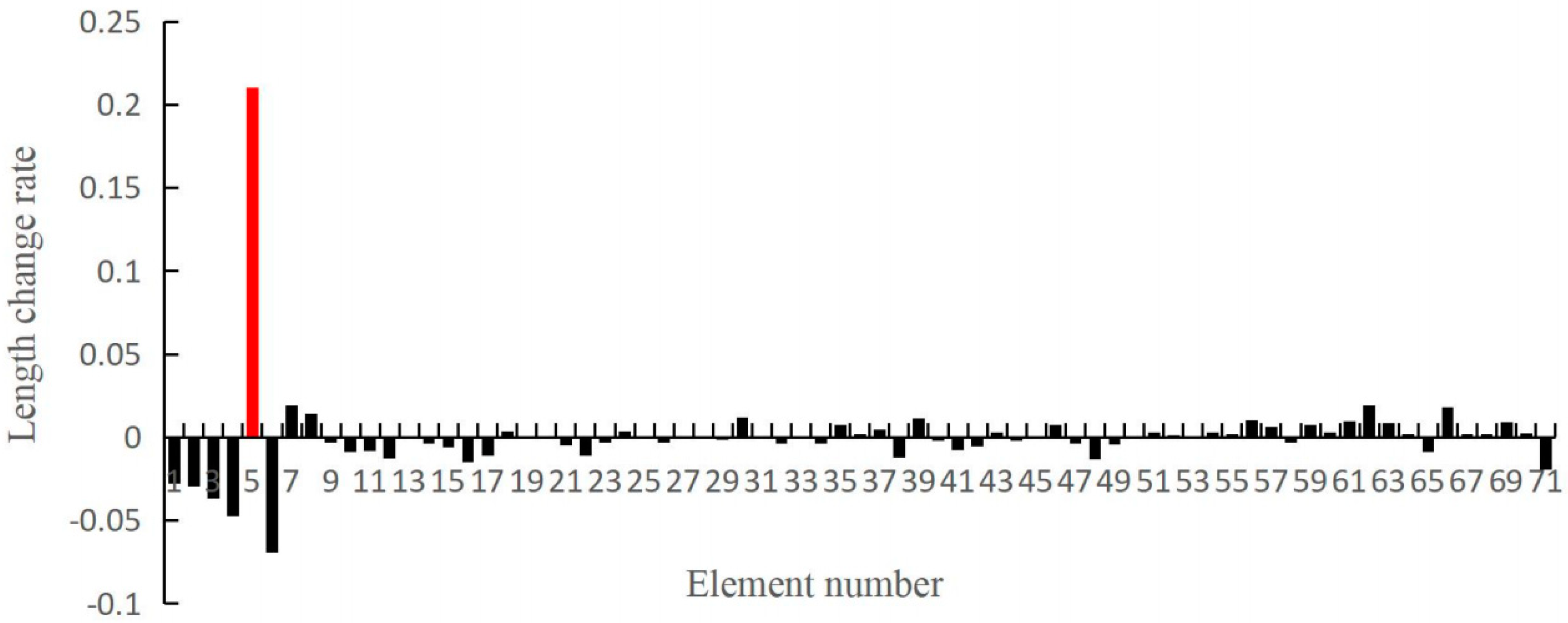
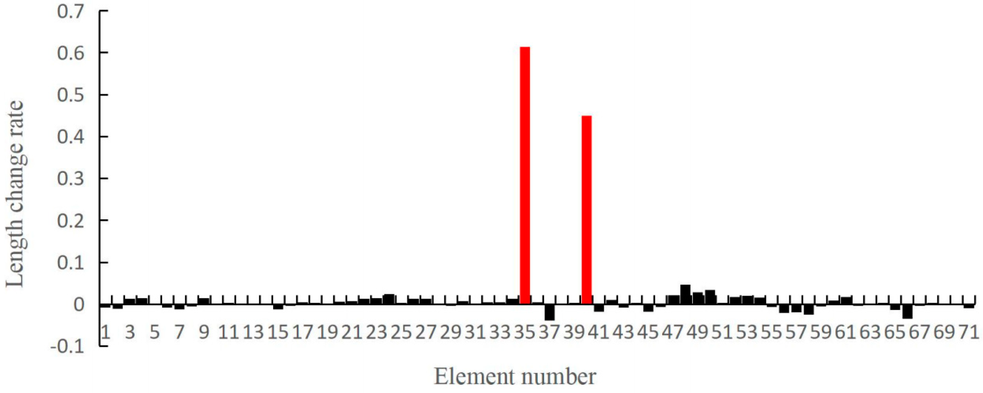
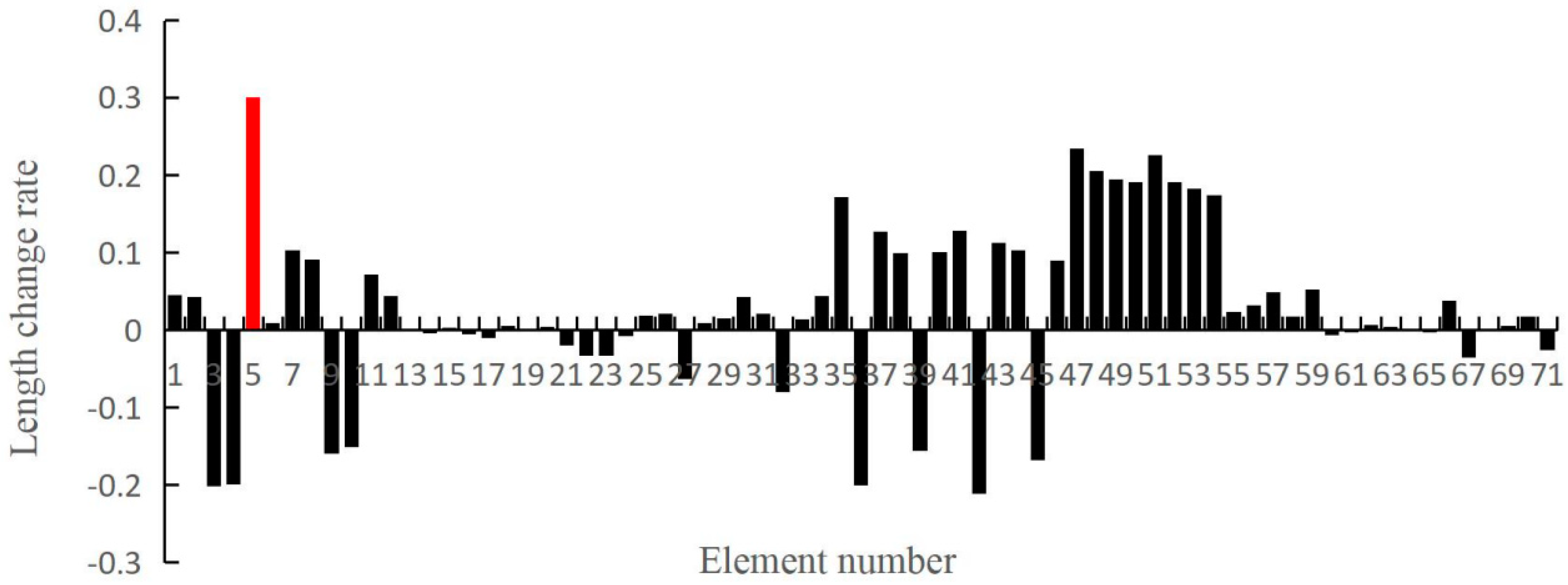
The rate of change of length ε of the element (strain) is calculated by Equation (19), and the element with the larger length change rate was identified as the position where the damage was most likely to occur.

4. Cases

The space grid structure in Figure 3 had a total of 71 elements. The main parameters were as follows: E = 200 GPa, ρ = 7.8 × 10³ kg/m³; A = 3.14 × 10⁻⁴ m²; L = 3 m. The three translational degrees of freedom were constrained at nodes 1, 7, 8, and 14, and a concentrated force of 20 kN in the negative Y-axis direction was applied at nodes 4 and 11, as shown in Figure 3a. In the example, the element damage was simulated by the reduction in elastic modulus.

Consider two cases of single damage and multiple damages: (1) simulate 20% stiffness damage for element 5 between nodes 5 and 6; and (2) simulate 20% stiffness damage for element 35 between nodes 1 and 15, and 20% stiffness damage for element 40 between nodes 7 and 19, respectively. First, we simulated the static test. According to the obtained static displacement data, under a concentrated force, the rates of length change of 71 elements before and after the damages occurred were calculated by Equation (15). The results obtained from the calculation without considering the noise are shown in Figure 4 and Figure 5.

It can be seen from Figure 4 and Figure 5 that when the data used were noise-free, the rate of change of length of the damaged element was abnormally increased, and the length change rates of the remaining elements were all small, indicating that the length change rate of the element was feasible as the basis for damage localization.

In order to test the noise resistance of the proposed method, data noise of 5% was added to the static displacement data to simulate the real measurement condition, and the results of the calculation using the noise-containing data are shown in Figure 6 and Figure 7. The formula for adding data noise is as follows:

$$\Delta u_{(j)}^{*}=\Delta u_{(j)}\times (1+nl\times unifrnd[-1,1])$$

(23)

where ∆u* denotes the jth component in the displacement change ∆u, ∆u*_(j) denotes the corresponding component contaminated with noise, unifrnd [−1, 1] denotes a random number in the range of −1 and 1, and nl denotes the noise level. As stated before, nl = 5% is used in this example.

As can be seen from Figure 6 and Figure 7, even if there was a noise interference of 5%, the damage of element 5 can be clearly judged from Figure 6, and the damage of elements 35 and 40 can be clearly judged from Figure 7. This indicates that the proposed method had good anti-noise ability.

As mentioned above, actual static loading may be difficult to perform on the actual engineering structure to obtain the displacement parameters. In such a case, a dynamic test can be used to obtain the modal parameters and the virtual displacement parameters. That is, a method that uses the dynamic flexibility combined with virtual force was adopted to obtain the displacement data indirectly. The results of the rate of length change of the element calculated by this method are shown in Figure 8, Figure 9, Figure 10 and Figure 11.

As seen in Figure 8 and Figure 9, in the case of no noise interference, the length change rate of the element obtained from the dynamic data can also determine the damage position of the element in a relatively clear manner. When there was 5% noise interference, as seen in Figure 10 and Figure 11, there was a significant peak at the position of the damaged element, which also indicated that the element with the larger length change rate was most likely to sustain damage. Note that the results obtained from the dynamic data were less accurate than those obtained from the static data. This is because the flexibility matrix obtained by the dynamic flexibility method was an approximation, and the displacement obtained by applying the virtual force based on this was naturally less accurate than that obtained from the direct static test. Therefore, in engineering practice, static conditions are preferred to obtain displacement parameters in order to obtain damage localization results with higher accuracy, when the conditions permit.

In order to study the sensitivity of the proposed method, Figure 12 and Figure 13 present the results of the elemental length change rates when element 44 (between nodes 12 and 22) was damaged with an added 5% noise. Specifically, Figure 12 gives the results when element 44 has 20%, 15%, and 10% stiffness reductions, and Figure 13 gives the results of 7.5% and 5% stiffness damages. From Figure 12, one can see that there was a significant peak at the damaged element 44, which indicated that the damage position can be determined in a relatively clear manner when the damage degree is more than 10%. The results in Figure 13 are confused, and it was impossible to accurately identify the true damage location, which indicated that the proposed method is ineffective when the damage degree is less than 10%. Obviously, the cause of misjudgment lies in the adverse effect of data noise, because the displacement changes caused by the damage are often submerged by the data noise when the damage degree is very small. For this case, 10% stiffness reduction is the minimum detectable damage.

5. Conclusions

We deduced the relationship between the characteristic force and characteristic displacement of the grid structure. The SMW formula was used to deduce the physical principle of damage identification by the displacement difference in detail. Based on this principle, the rate of length change of the element was proposed to implement the identification of damage position in the grid structure. A space grid structure was taken as an example. A numerical example was used to verify the result. The result indicated that the element with larger length change rate was the most likely position where damage occurred. The proposed method has certain noise resistance and can obtain better identification effects in the case of single or multiple element damage. The biggest advantage of the proposed method is that it is not necessary to establish a finite element model. In the specific application of the project, the displacement difference can be calculated only by a static test, such as using a laser range finder to obtain the displacement data of each node in order to calculate the displacement difference. If the static displacement data cannot be obtained directly, it can be obtained from the parameters obtained by dynamic testing. Therefore, the proposed method has good prospects for application.

References

1. Li, C.H.; Yang, Q.W.; Sun, B.X. A Virtual Load Method for Damage Identification of Beam Structures. Recent Pat. Eng. 2018, 12, 117–126. [Google Scholar] [CrossRef]
2. Yang, Q.W.; Wang, C.; Li, N.; Wang, W.; Liu, Y. Enhanced Singular Value Truncation Method for Non-Destructive Evaluation of Structural Damage Using Natural Frequencies. Materials 2019, 12, 1021. [Google Scholar] [CrossRef] [PubMed]
3. Zhu, H.; Yu, J.; Zhang, J. A summary review and advantages of vibration-based damage identification methods in structural health monitoring. Eng. Mech. 2011, 28, 1–17. [Google Scholar]
4. Yin, Z.; Wang, W.; Jiao, D. Experiment and simulation analysis of damage of space truss. J. Civ. Arch. Env. Eng. 2017, 39, 78–84. [Google Scholar]
5. Wang, M.; Song, C.; Ji, C. Research on damage detection method for grid structures based on frequency response function and principal component analysis. Build. Struct. 2017, 47, 96–101. [Google Scholar]
6. Li, H.; Lin, S.; Yi, T. Study on Structural Damage Identification by Static Virtual Distortion Method. J. Arch. Civ. Eng. 2016, 33, 1–6. [Google Scholar]
7. Yu, O.; Chao, X.; Yang, W. A Two-Stage Method for Beam Damage Identification Based on Static Deflection. Chin. Q. Mech. 2017, 38, 458–467. [Google Scholar]
8. Huang, B.; Zong, R.; Yang, T. Damage Identification of Random Beam Structure Based on Static Measurement Data. Chin. J. Comput. Mech. 2013, 180–185. [Google Scholar] [CrossRef]
9. Huang, B.; Guo, W.; Lu, Y. An Improved Method for Static Damage Identification of Random Beam Structures. Chin. J. Comput. Mech. 2018, 21, 451–456. [Google Scholar]
10. Hosseinzadeh, A.; Ghodrati, A.G.; Koo, K.Y. Optimization-based method for structural damage localization and quantification by means of static displacements computed by flexibility matrix. Eng. Optim. 2016, 48, 543–561. [Google Scholar] [CrossRef]
11. Mehrisadat, M.; Alamdari, L.; Ge, K.; Zhou, K.Y.; Du, Z. Non-contact structural health monitoring of a cable-stayed bridge: Case study. Struct. Infrastruct. Eng. 2019, 15, 1119–1136. [Google Scholar]
12. Chen, Z.H.; Zhu, S.; Xu, Y.; Li, Q.; Cai, Q. Damage Detection in Long Suspension Bridges Using Stress Influence Lines. J. Bridge Eng. 2015, 20, 05014013. [Google Scholar] [CrossRef]
13. Kawano, A.; Zine, A. Reliability evaluation of continuous beam structures using data concerning the displacement of points in a small region. Eng. Struct. 2019, 180, 379–387. [Google Scholar] [CrossRef]
14. Mao, Q.; Mazzotti, M.; DeVitis, J. Structural condition assessment of a bridge pier: A case study using experimental modal analysis and finite element model updating. Struct. Control Health Monit. 2018, 26, e2273. [Google Scholar] [CrossRef] [Green Version]
15. Pu, Q.; Hong, Y.; Chen, L. Model updating-based damage detection of a concrete beam utilizing experimental damped frequency response functions. Adv. Struct. Eng. 2019, 22, 935–947. [Google Scholar] [CrossRef]
16. Astroza, R.; Alessandri, A. Effects of model uncertainty in nonlinear structural finite element model updating by numerical simulation of building structures. Struct. Control Health Monit. 2019, 26, e2297. [Google Scholar] [CrossRef]
17. Yang, Q.W.; Du, S.G.; Liang, C.F. A Universal Model-Independent Algorithm for Structural Damage Localization. Comput. Modeling Eng. Sci. 2014, 100, 223–248. [Google Scholar]
18. Feng, D.; Feng, M.Q. Computer vision for SHM of civil infrastructure: From dynamic response measurement to damage detection A review. Eng. Struct. 2018, 156, 105–117. [Google Scholar] [CrossRef]
19. Feng, D.; Feng, M.Q. Model Updating of Railway Bridge Using in Situ Dynamic Displacement Measurement under Trainloads. J. Bridge Eng. 2015, 20, 04015019. [Google Scholar] [CrossRef]
20. Qin, J.; Gao, Z.; Wang, X.; Yang, S. Three-Dimensional Continuous Displacement Measurement with Temporal Speckle Pattern Interferometry. Sensors 2016, 16, 2020. [Google Scholar] [CrossRef]
21. Hung, Y.Y. Displacement and Strain Measurement; Dekker: New York, NY, USA, 1978; Volume 4, pp. 51–71. [Google Scholar]
22. Lee, J.J.; Shinozuka, M. Real-time displacement measurement of a flexible bridge using digital image processing techniques. Exp. Mech. 2006, 46, 105–114. [Google Scholar] [CrossRef]
23. Feng, D.; Feng, M.; Ozer, E. A vision-based sensor for noncontact structural displacement measurement. Sensors 2015, 15, 16557–16575. [Google Scholar] [CrossRef] [PubMed]
24. Twu, R.C.; Yan, N.Y. Immersion-type KTP sensor for angular displacement measurement. Opt. Laser Technol. 2019, 120, 105690. [Google Scholar] [CrossRef]
25. Kondo, T.; Suzuki, Y.; Matoba, K. Displacement measurement device, measurement system, and displacement measurement method. U.S. Patent Application 15/893,702, 28 March 2019. [Google Scholar]
Figure 1. Grid structure with 11 elements.
Applsci 09 03252 g001
Figure 2. Force of element 3 (Fr is resultant force).
Applsci 09 03252 g002
Figure 3. (a). X-Y axis elevation structure and force; (b). Standard view of the space grid structure of element.
Applsci 09 03252 g003
Figure 4. Rate of change of element length obtained from the static data (element 5 had damage with no noise).
Applsci 09 03252 g004
Figure 5. Rate of change of element length obtained from the static data (elements 35 and 40 were damaged with no noise).
Applsci 09 03252 g005
Figure 6. Length change rate of element obtained from the static data (element 5 was damaged with an added 5% noise).
Applsci 09 03252 g006
Figure 7. Length change rate of element obtained from the static data (elements 35 and 40 were damaged with an added 5% noise).
Applsci 09 03252 g007
Figure 8. Length change rate of element obtained from the dynamic data (element 5 was damaged with no noise).
Applsci 09 03252 g008
Figure 9. Length change rate of element obtained from the dynamic data (elements 35 and 40 were damaged with no noise).
Applsci 09 03252 g009
Figure 10. Length change rate of element obtained from the dynamic data (element 5 was damaged adding 5% noise).
Applsci 09 03252 g010
Figure 11. Length change rate of element obtained from the dynamic data (elements 35 and 40 were damaged adding 5% noise).
Applsci 09 03252 g011
Figure 12. Length change rate of element obtained from the static data with an added 5% noise (element 44 has 20%, 15%, and 10% stiffness reductions).
Applsci 09 03252 g012
Figure 13. Length change rate of element obtained from the static data with an added 5% noise (element 44 has 7.5% and 5% stiffness reductions).
Applsci 09 03252 g013