Article

Blind Image Deblurring Based on Local Edges Selection

1
School of Technology, Beijing Forestry University, No.35 Tsinghua East Road, Haidian District, Beijing 100083, China
2
Key Laboratory of State Forestry Administration on Forestry Equipment and Automation, No.35 Tsinghua East Road, Haidian District, Beijing 100083, China
*
Author to whom correspondence should be addressed.
Appl. Sci. 2019, 9(16), 3274; https://doi.org/10.3390/app9163274
Submission received: 22 July 2019 / Accepted: 6 August 2019 / Published: 9 August 2019
(This article belongs to the Section Computing and Artificial Intelligence)

Abstract

:
The edges of images are less sparse when images become blurred. Selecting effective image edges is a vital step in image deblurring, which can help us to build image deblurring models more accurately. While global edges selection methods tend to fail in capturing dense image structures, the edges are easy to be affected by noise and blur. In this paper, we propose an image deblurring method based on local edges selection. The local edges are selected by the difference between the bright channel and the dark channel. Then a novel image deblurring model including local edges regularization term is established. The obtaining of a clear image and blurring kernel is based on alternating iterations, in which the clear image is obtained by the alternating direction method of multipliers (ADMM). In the experiments, tests are carried out on gray value images, synthetic color images and natural color images. Compared with other state-of-the-art blind image deblurring methods, the visualization results and performance verify the effectiveness of our method.

1. Introduction

Image deblurring has long been a challenging problem. The aim of image deblurring is to recover a clear image from a blurred image. Image deblurring can be separated into non-blind and blind cases. In non-blind image deblurring, the blurring kernel is known in advance and the clear image is obtained from the blurred image and blurring kernel [1,2,3]. Different from non-blind image blurring, blind image deblurring aims to obtain a clear image from a blurred image when the blurring kernel is unknown. Generally, the uniform blurring process [4] is modeled by:
y = H x + n
where y is the blurred image, H is the blurring kernel, x is the clear image, n is additive noise, and is the convolution operator.
Blind image deblurring is an ill-posed problem, in which clear image and blurring kernel are unknown. Given a blurred image, there are countless sets of estimated results on clear images and blurring kernels. Researchers have been working for many years to estimate better results for clear image and blurring kernel [5,6,7,8,9]. Many state-of-the-art image deblurring algorithms solve the ill-posed problem within the maximum a posteriori (MAP) framework [5]. In MAP based image deblurring methods, the process of estimating clear image can be formulated as follows:
p ( x , H | y ) = p ( y | x , H ) p ( x ) p ( H ) p ( y )
where p ( x ) and p ( H ) are the probability density functions of clear image and blurring kernel. In image deblurring, p ( y ) is known in advance, so Equation (2) can be can be simplified as follows:
p ( x , H | y ) p ( y | x , H ) p ( x ) p ( H )
where p ( y | x , H ) , p ( x ) , and p ( H ) are the likelihood term, the priors on the clear image, and the priors on the blurring kernel, respectively [5]. According to Equation (3), the image deblurring model [6] can be summarized as follows:
( x * , H * ) = a r g m i n x , H P ( y , x , H ) + Q ( x ) + R ( H )
where P, Q, and R are the likelihood term, the regularization term based on image priors, and the regularization term based on the blurring kernel, respectively. The likelihood term is usually formulated as follows [6]:
P ( y , x , H ) = y x H 2 2
The regularization term Q ( x ) is built based on a large number of experiments on image priors [7,8,9]. R ( H ) is often formulated by the Lp-norm of H [7,8,9,10].
Numerous image deblurring algorithms have been proposed in the past years. Some of them use the sparse priors on natural images [7,9,10,11,12,13], but the statistical priors on image or image gradients are not effective for all kinds of images [8]. The edges of an image are less sparse when the image becomes blurred [14], so some algorithms focus on building deblurring models by using the salient image edges. Joshi et al. [15] found the location and orientation of edges by a sub-pixel difference of Gaussians edge detector, then predicted sharp edges by propagating the maximum and minimum values along the edge profile. Jia [16] estimated the blurring kernel by using the transparency on the image boundary. Hu et al. [17] stated that smooth regions cannot contribute much for estimating the ground truth of the kernel, and proposed a method to extract suitable regions for blurring kernel estimation. Javaran et al. [18] extracted the main structure of the blurred object, then selected salient edges by shock filtering. Cho and Lee [19] obtained image salient edges by bilateral filtering. Xu and Jia [20] proposed a deblurring method in which the edges selection method is also based on shock filtering. In [21], color image gradients were added in the likelihood term instead of other operators. However, in these methods, the image edges are selected based on the global information of the image, the dense structures cannot be captured, and the edges are easy to be affected by noise [4]. In addition, when image become blurred, it is even harder to extract image edges well by these methods. Recently, image restoration methods based on deep learning [22,23] and super resolution [24,25,26] are proposed, which can obtain good results when applied to image deblurring. However, a large number of computations are needed, or a lot of images are required for training, which add to the complexity of the algorithm.
Considering the limitation of global edges of images, we propose a new blind image deblurring method based on local edges selection. The contributions of the proposed method are summarized as follows:
(1)
The proposed image deblurring model is built based on MAP, but different from traditional MAP based methods, in the deblurring model, we add creative local image edges, the local edges are selected from the bright and dark channels of the image.
(2)
In most blind image deblurring methods, the blurring kernel is estimated first and the clear image is obtained by non-blind deblurring methods. Different from these methods, the clear image and blurring kernel are obtained based on alternating iteration in the proposed method.
(3)
Tests are carried out based on the dataset of gray value images, color images, and natural color images. The experimental results show that the proposed method can effectively deblur different kinds of images. By comparing with other state-of-the art methods in visual results and quantitative matrices, the clear image and blurring kernel results verify the effectiveness of the proposed method.
The rest of this paper is organized as follows. Section 2 consists of five parts. In Section 2.1, the proposed local edges selection method is introduced. Then the image deblurring model and blind deblurring process are introduced in Section 2.2. In Section 2.3 and Section 2.4, we present the estimation of the blurring kernel and clear image, respectively. Section 2.5 introduces the stopping criterion. Section 3 provides image deblurring results and discussions, consisting of four parts. The results of image edges selection are shown in Section 3.1. In Section 3.2 and Section 3.3, we discuss the parameters in the deblurring model and the convergence of the proposed algorithm. In Section 3.4, we provide the results of the image deblurring we carried out, and compare the images deblurring results with other state-of-the-art methods to verify the effectiveness of the proposed method. Finally, Section 4 is the conclusion of this paper.

2. Method

2.1. Local Edges Selection Method

Traditional methods obtain image edges by global filtering. Gradient filters consider two or three pixels in the neighborhood, which tends to ignore longer range dependencies [4]. In contrast, image patches can model more complex image structures in larger neighborhoods [27]. So recently some patch-based image deblurring methods are proposed, such as image deblurring based on patch priors [4,28] and internal patch recurrence [27], etc. The dark channel [29] and bright channel [30] are useful matrices based on local information of image, some previous methods use them in haze removal [29] and image restoration [30,31]. Different from all these methods, in this paper, we innovatively select image edges by using dark channel and bright channel, and build the deblurring model.
Dark channel [29] is obtained by finding the minimum value in an image patch, which is defined as follows:
Φ 1 x w = min u N ( w ) min c R , G , B x c u
where Φ1(x) is the dark channel of x, N ( w ) is an image patch centered at w, and xc is the cth channel of the RGB color image. Similarly, the bright channel [31] represents the maximum value in an image patch, which is defined as follows:
Φ 2 x w = max u N ( w ) max c R , G , B x c u
Based on the bright channel and dark channel, we propose a new image edges selection method. The edge of an image is composed of points whose brightness changes obviously, so the edge of an image can also be regarded as the junction of the “bright” area and the “dark” area. By subtracting the bright channel image from the dark channel image, the complete edges of an image can be obtained. So in the proposed method, the edges of image x can be obtained as follows:
x ^ = Φ 2 x Φ 1 x
The proposed method can select the edges of color images as well as gray value images. In Equations (6) and (7), when the input image is a gray-value image, the dark channel and bright channel can be obtained by Equations (9) and (10):
Φ 1 x w = min u N ( w ) x c u
Φ 2 x w = max u N ( w ) x c u

2.2. Image Deblurring Model

As is mentioned above, the edges of images are less sparse when the image become blurred. Based on the changes in sparsity, in some methods, the first-order or higher-order gradient operators are added to the deblurring model in likelihood terms [19]; some methods also find new criteria for selecting informative edges [20], but adding too many partial derivative operators will increase computational complexity and reduce efficiency [21]. In addition, sometimes the failure of extracting blurred image edges will cause ringing artifacts. Since the proposed edges selection method can better detect the edges of the image, we use it to build the deblurring model.
The proposed image deblurring model is defined as follows:
arg min x , H y H x 2 2 + y ^ H x ^ 2 2 + α Q T V ( x ) + β H 2 2
where x ^ and y ^ are the local edges of clear image and blurred image. QTV(x) is the optimized total variation term and Section 2.4 covers it in detail.
Then, based on the proposed deblurring model, the image deblurring process is shown in Algorithm 1. The blurred image y and the blurring kernel size are the input, the output values of the algorithm are the clear image x and blurring kernel H. In the initial stage of the algorithm, the clear image x and blurring kernel H are unknown, so we need to initialize them. In the proposed method, we initialize clear image x by setting x = y. The blurring kernel H is assumed to be a sparse matrix and a few pixels are nonzero [21] in the initialization. In subsequent calculations, the value of x and H are constantly updated in each iteration until the algorithm stops. In each iteration, we obtain the renewed local edges of the intermediate clear image x by the proposed local edges selection method, then the intermediate clear image and blurring kernel are renewed respectively. When the stopping criterion is satisfied, we can get the final results of the clear image and blurring kernel. The stopping criterion is introduced in Section 2.5.
Algorithm 1. The blind image deblurring process
1.  Input: blurred image y, kernel size [m,n]
2.  Initialization: x = y; H = zeros [m,n], H (1,1) = 1; KS = 0;
3.  if KS ≤ 0.95
  Estimate intermediate clear image x by the method in Section 2.4;
  Estimate intermediate blurring kernel H by the method in Section 2.3;
  Update kernel similarity (KS) by the method in Section 2.5;
4.  or else break;
5.  Output: x, H

2.3. Estimation of Blurring Kernel

In the proposed method, the blurring kernel is obtained by Equation (12). Because of the effectiveness of the proposed edges selection method, we do not make more constraints on the blurring kernel. So, in each iteration, the intermediate blurring kernel in Algorithm 1 can be easily obtained by the fast Fourier transform (FFT) method, which is defined in Equation (13).
arg min H y H x 2 2 + y ^ H x ^ 2 2 + β H 2 2
H = F 1 F ( x ^ ) F T ( y ^ ) + F ( y ^ ) F T ( x ^ ) + F ( x ) F T ( y ) + F ( y ) F T ( x ) F ( x ^ ) F T ( x ^ ) + F ( x ) F T ( x ) + β
where y ^ and x ^ are the edges selected by the proposed method, and x is the intermediate result of clear image in the previous iteration. F ( ) and F 1 ( ) are the forward and inverse Fourier transforms, respectively, and F T ( ) is the complex conjugate of F ( ) .

2.4. Estimation of Clear Image

In the estimation of the clear image, we aim to solve the function as follows:
arg min x y H x 2 2 + y ^ H x ^ 2 2 + α Q T V ( x )
Q T V ( x ) = i = 1 4 i x 2
where i is the image gradients filter [32] in the directions of 0°, 45°, 90°, and 135°; different from the method in [32], the operators are obtained by bilinear interpolation of the basic gradients operator [21]. In fact, when i = 2, i comprises the image gradient operators in the directions of 0° and 90°, then Q T V ( x ) represents the classic total variation [33]. We add two more directions based on the total variation term to reduce ringing artifacts.
The dark channel and bright channel are obtained by a non-linear operation. In the method proposed by Pan et al. [31], dark channel is equivalently transformed into the multiplication of the image and a linear operator, then the clear image can be achieved by FFT method. However, in Pan’s method, the linear operator is obtained by using gray value image rather than color image, so it is not the best way to solve the problem by introducing a linear operator. In the proposed method, the clear image is obtained within the alternating direction method of multipliers (ADMM) framework [32], where the clear image can be achieved as follows:
x = F 1 F T ( H ) a k + b k F ( H ) F T ( H ) + i = 1 4 F T ( i ) c k + d k F ( i ) F T ( i )
where k is the inner iteration time. With a k , b k , c k and d k as intermediate parameters, the process of obtaining clear image is as follows:
In Algorithm 2, a k and c k are obtained by the gradient descent method [14]. In each iteration, a k , b k , c k and d k are obtained first, then intermediate image xk are obtained by Equation (16). When iteration time reaches 20, the algorithm can converge to a high accuracy, so we empirically set k = 20. The detailed convergence analysis is introduced in Section 3.3.
Algorithm 2. The calculation of clear image
1. Initialization: x0, H (Intermediate results in the previous iteration); a0, b0, c0, d0
2. for k = 1:20
3. Calculate
a k = arg min x k H x k + x ^ k y + y ^ x k 1 + x ^ k 1 b k 1 2 2
b k = a k + b k 1 H x k y 2 2
c k = arg min x k i = 1 4 i x k d k 1 x k 1 2 2 + x k 2 2
d k = d k 1 + c k i = 1 4 i x k 2 2
4. Obtain xk by Equation (16)
5. end
6. x = x20

2.5. Stopping Criterion

In the proposed method, the intermediate clear image and blurring kernel are alternately obtained in each iteration. With the iteration time increases, the estimated intermediate clear image and blurring kernel are closer to the real ones. When the iteration time reaches a certain number, the results converge to a higher accuracy, and the iteration can be stopped. In the proposed method, we utilize the kernel similarity to decide the stopping criterion. Kernel similarity [17] is defined as follows:
K S ( H , H 1 ) = max γ τ H ( τ ) H 1 ( τ + γ ) | | H | | | | H 1 | |
where H is the real kernel, H1 is the intermediate estimated kernel. The value of kernel similarity ranges from 0 to 1, the larger value of kernel similarity reflects the better result.
In the proposed method, we set H and H1 to be the estimated kernel in two contiguous iterative processes. In the first few iterations, the kernel similarity changes largely. After a certain number of iterations, the change of blurring kernel tends to be slow, then kernel similarity increases. After exhaustive experiments, the stopping criterion of the proposed method can be summarized as follows: After the iteration number reaches 10, when the kernel similarity is between H and H1 higher than 0.95, the iteration stops.

3. Results and Discussion

3.1. The Results of Image Edges Selection

First, tests are carried out to verify the effectiveness of the proposed edges selection method. Figure 1 shows the comparison of different edges selection methods. It can be seen from Figure 1 that the first-order image gradients [9] and Laplace gradients cannot effectively represent the edges well in each direction. Although Canny edges selection method [34] can better extract the details of image edges, its thinning operation on image edges will bring unnecessary noise to the image. In contrast, the proposed method can get more complete and smooth image edges in each direction. Moreover, because the proposed edges selection method is based on image patch, it also has rotation invariance. Figure 1e shows the edges of gray value images obtained by the proposed method whose dark channel and bright channel are calculated by Equations (9) and (10). We can see from Figure 1e that the proposed method can select image edges effectively. Figure 1f is the edges of color images, and Φ1(x), Φ2(x) are calculated by Equations (6) and (7). The method utilizes the color information of the image, and the selected edges are more representative than the edges in Figure 1e. It can be concluded from the test that the proposed edges selection method based on local information is more effective than others. In addition, salient edges and detailed texture information can be better obtained using color information.
The proposed edges selection method is also applicable to blurred images. Figure 2 shows the comparison of the selected edges in a patch of the image in Figure 1. In the comparison methods, image gradients are obtained by using the difference between adjacent pixels. When the image becomes blurred, image structure becomes blurred as well, the difference between adjacent pixels is not so large near image edges, so edges cannot be extracted well. In contrast, the proposed edges selection method can preserve image structure as much as possible, and can avoid bringing unnecessary noise.

3.2. Discussion of the Parameters in the Deblurring Model

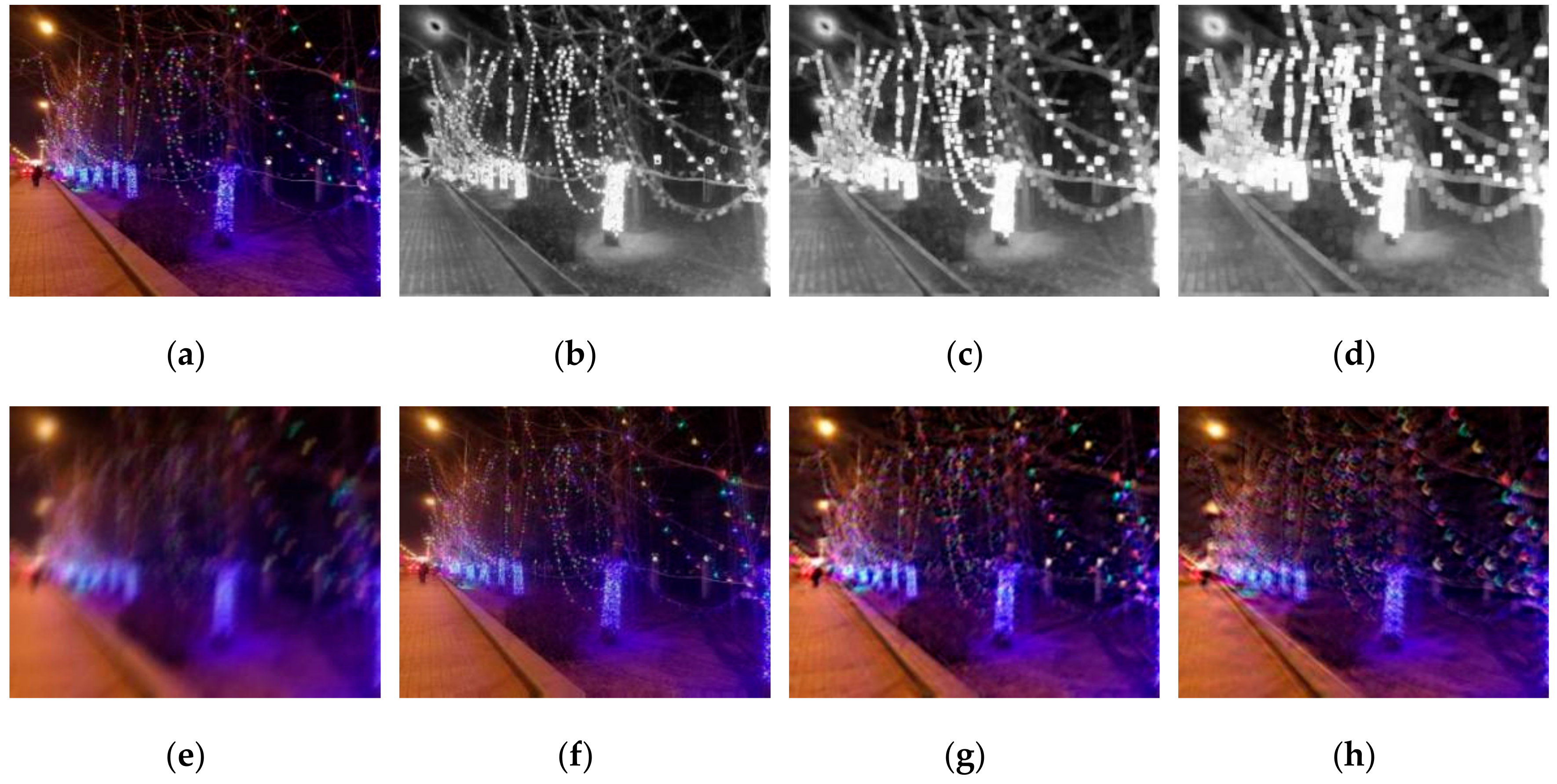
In this subsection, we will discuss how the parameters in the model effect the deblurring results. First, the size of local image patch will affect the edges selection results and the final image deblurring results. When the size of the image patch N ( w ) in Formulas (6) and (7) is less than 9 × 9, for normal images, it nearly has no influence on the deblurring results. However, for low illumination images or saturated images, when choosing larger sizes of image patches, the edges cannot be selected well, thus leading to bad kernel estimating results. Figure 3 shows an example of how the window size influence the deblurring result. Based on exhaustive experiments, we set the patch size to be 5 × 5.
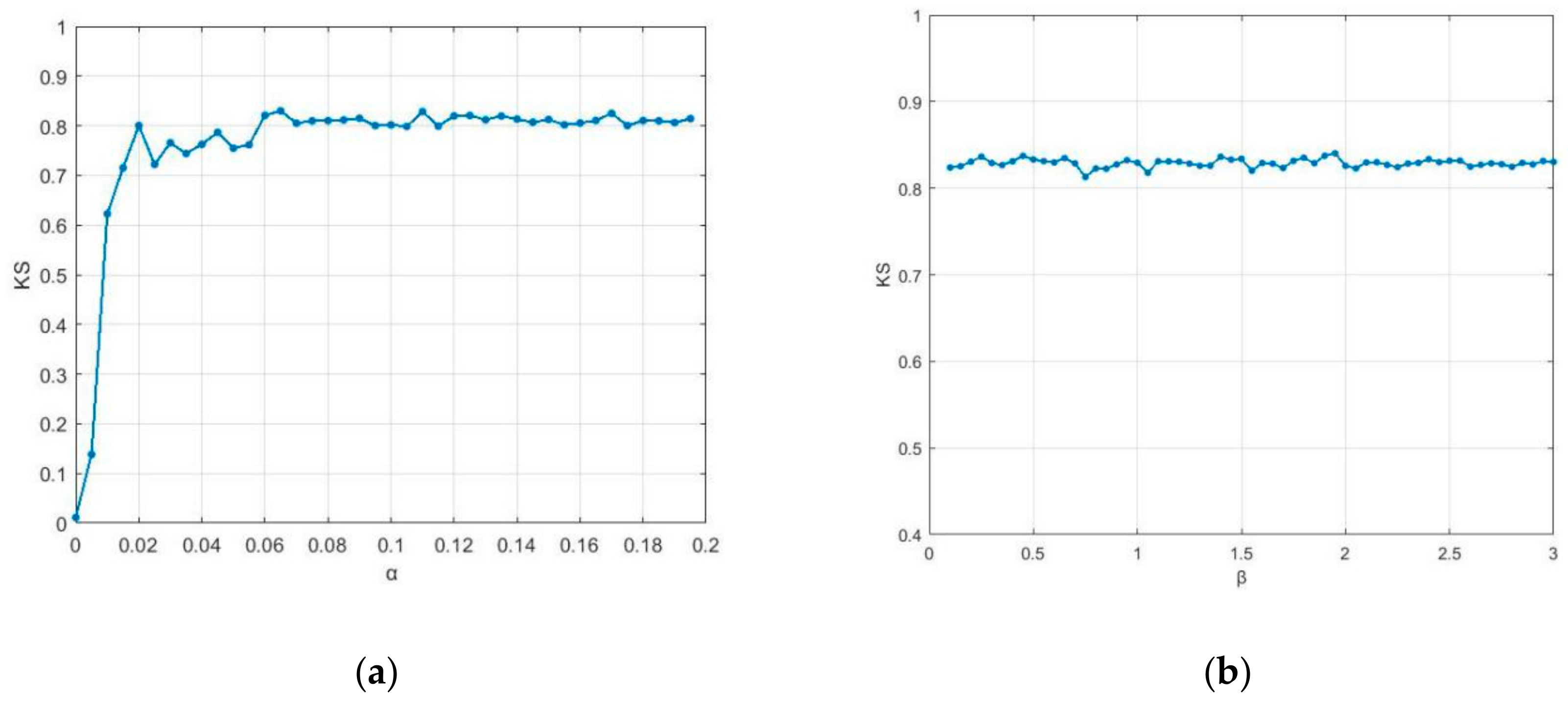
In addition, the proposed model involves two parameters, α and β . In order to analyze the effects of the two parameters on the proposed image deblurring method, we test the sensitivity of α and β . The sensitivity analysis is similar to the method proposed by Pan et al. [8]. In the analysis of each parameter, other parameters remain unchanged. We set the value of α from 0.0001 to 0.2 with the step size of 0.005, the value of β ranges from 0.1 to 3 with the step size of 0.05. In the sensitivity analysis test, kernel similarity is the metric to measure the accuracy of estimated kernels. Figure 4 shows the average kernel similarity of the 20 test images in the test, and the results show that the proposed method performs well with a wide range of parameter settings, and the algorithm has certain robustness for parameter selection.

3.3. The Convergence

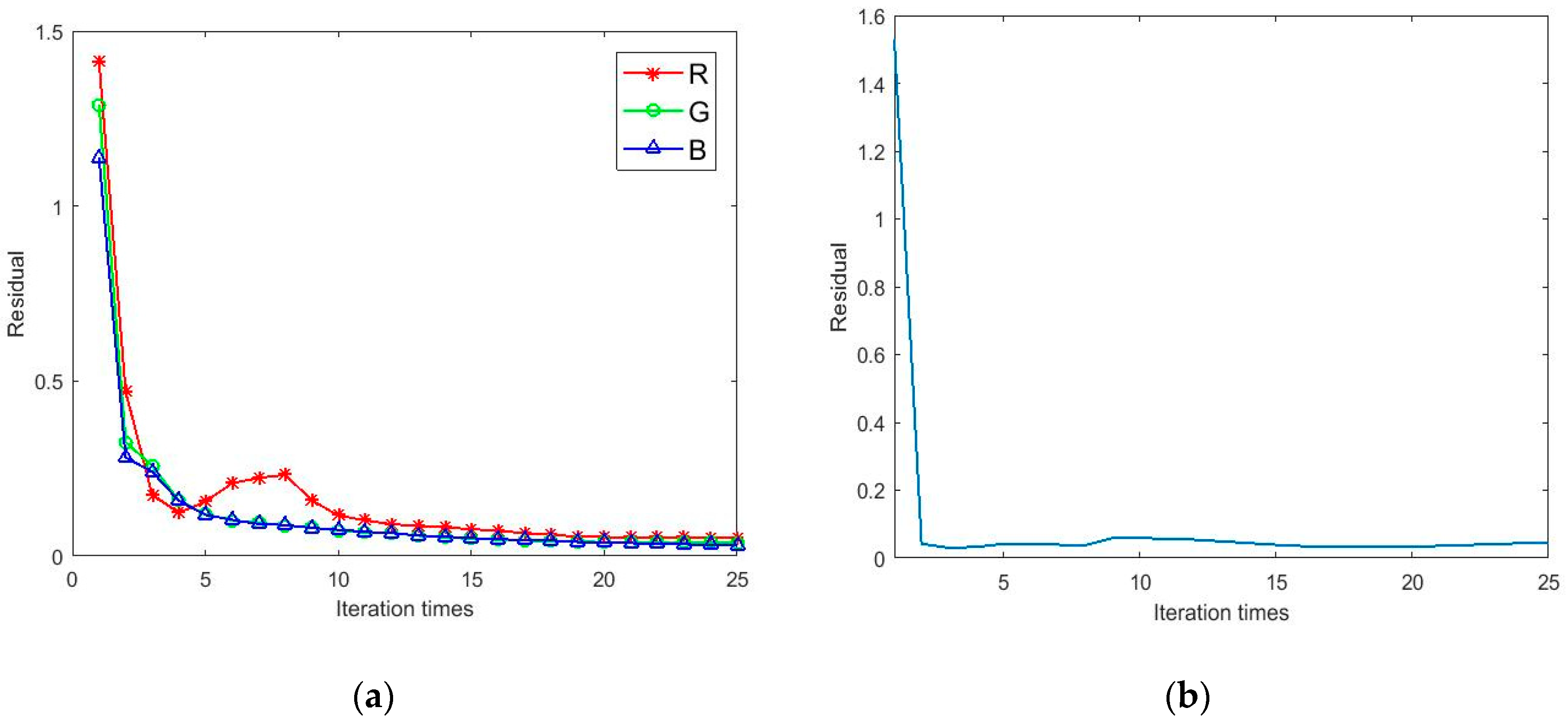
In order to verify the effectiveness of the proposed method, we test the convergence. Figure 5 shows the residual [35] of the proposed method with the iteration time increases. In Figure 5a, the residual of R, G, and B channel are calculated respectively, of the color image. Figure 5b shows the residual of blurring kernel. With the iteration time increases, the residual [23] gradually reduces. When the iteration reaches 20, the proposed algorithm can converge to a high precision, so the inner iteration times of the image and blurring kernel are set to be 20 in the deblurring process. From the convergence test, we can conclude that the proposed algorithm can converge to the real results of clear image and blurring kernel with high probability.

3.4. Image Deblurring Results

In all the tests, the size of the image patch N(w) equals 5 × 5. The parameters in Formula (11) are set to be the same in all the experiments: α = 0.008 , β = 0.7 . The parameters of the comparison methods in this section are selected according to the references.
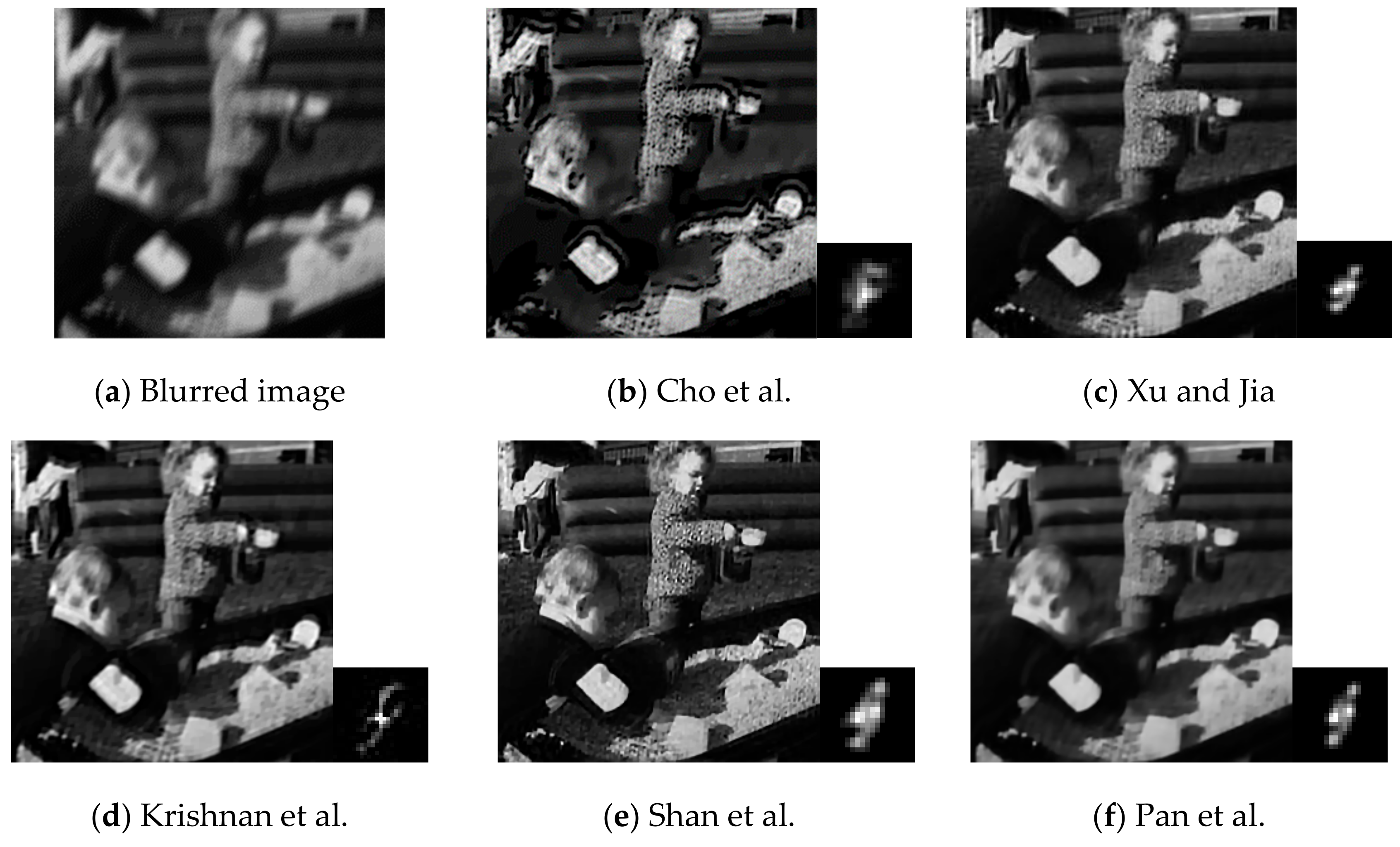
The first test is based on the dataset of Levin [5] which is shown in Figure 6—the blurred images are obtained by using eight blurring kernels and four ground truth gray value images. In the deblurring of gray value images, the dark channel and bright channel are obtained by Equations (9) and (10). The comparison algorithms include the methods in [7,9,19,20,22,27,31,33,36]. Figure 7 shows the visual results of one motion blurred image in Levin’s dataset. From the estimated clear images, the proposed method outperforms others. The clarity of the estimated clear images by some methods are relatively poor, such as [7,19]. The clear images obtained by the methods in [22,31] are too smooth, which may lead to the loss of some details. The brightness of the image has changed a lot in the image obtained by [36]. The blurring kernels estimated by the proposed method are also closer to the real kernels and have fewer noise points. Table 1 shows quantitative comparison results of the clear image and blurring kernel in Figure 7, the metrics include structure similarity (SSIM) [37], Peak Signal to Noise Ratio (PSNR) [38] and kernel similarity (KS). It can be seen from the results that the proposed method outperforms competing methods.
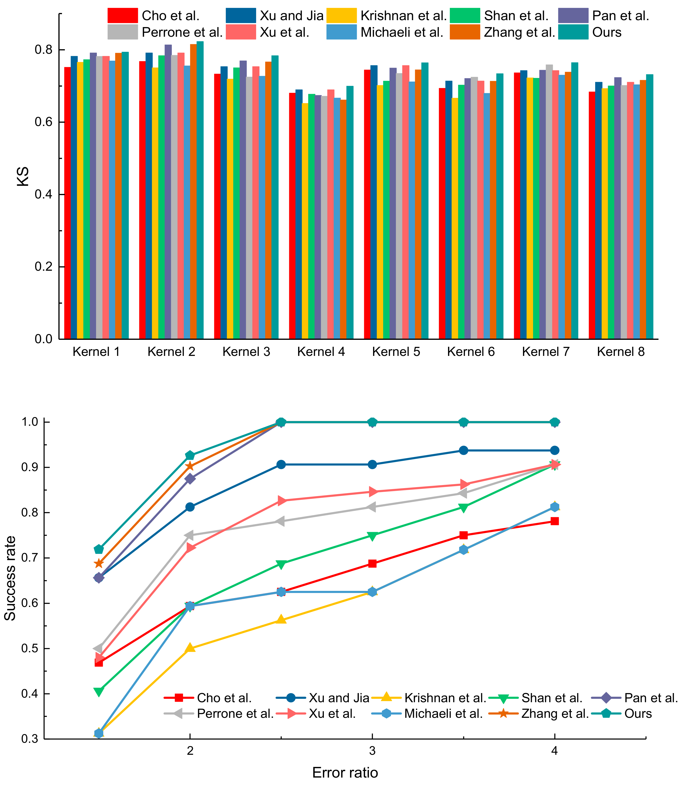
Then, tests are carried out based on all the 32 synthetic blurred images in Levin’s dataset. In addition to SSIM, PSNR, and KS, success rates are obtained based on the dataset. The success rate is measured by error ratio [5], which is defined in Equation (18), x p e , x p t are the clear images obtained by the estimated blurring kernel and the ground truth blurring kernel, respectively, for each pixel p . x p g is the ground truth clear image for each pixel p . Empirically, when the error ratio is lower than 3, the algorithm is considered to be successful. Figure 8 shows the average SSIM, PSNR, KS, and success rate. From the comparison results, the proposed method can deblur the gray value images well, and all the indices are dominant among the methods. In the proposed method, when the error ratio equals to 2.5, the success rate reaches 100%, and the proposed method outperforms others consistently.
r = p x p e x p g 2 2 p x p t x p g 2 2
Then, experiments are carried out based on the 48 color images in the dataset of Köhler et al. [39], which includes four ground truth color images and 12 blurring kernels. The 48 synthetic images in Köhler’s dataset are deblurred by the proposed method and other methods in [1,7,9,19,20,22,31,40,41,42]. Figure 9 shows the visualization results of one blurred image in the dataset. The results show that the proposed method can effectively restore detailed information of images. Some methods cannot obtain clear images successfully, the image is still suffered from serious blur, such as [1,41]; In some deblurring images, such as the images estimated by [7,19,20,22], ringing artifacts affect the deblurred results. It can be seen more clearly from the magnified views that the ringing artifacts are better suppressed by the proposed method, and the estimated image is clearer than others. Then, quantitative comparisons are carried out based on the 48 images in Köhler’s dataset. Figure 10 shows the comparisons of the average SSIM and PSNR values. The proposed method outperforms others in quality indices—the SSIM and PSNR are consistently higher than others.
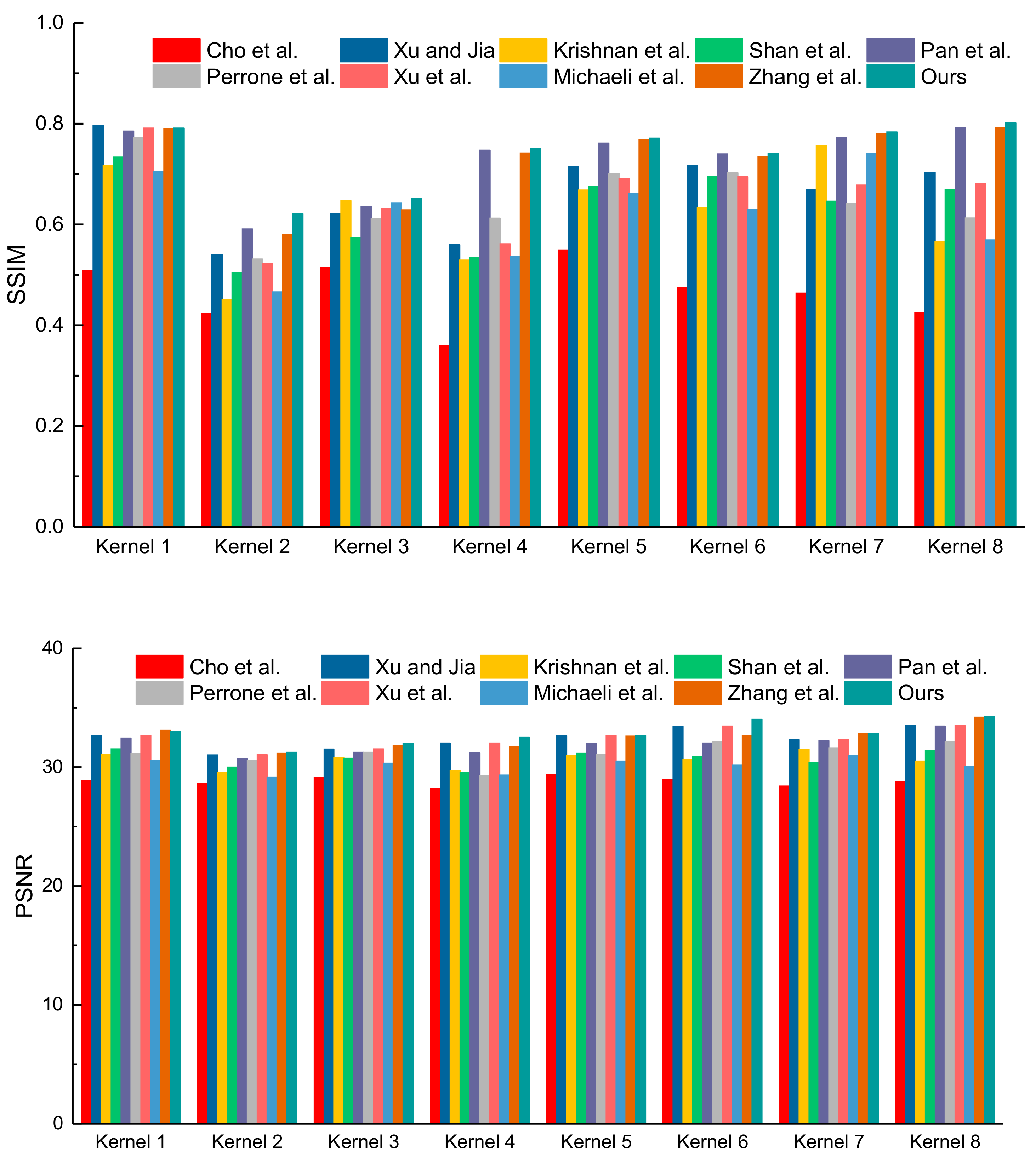
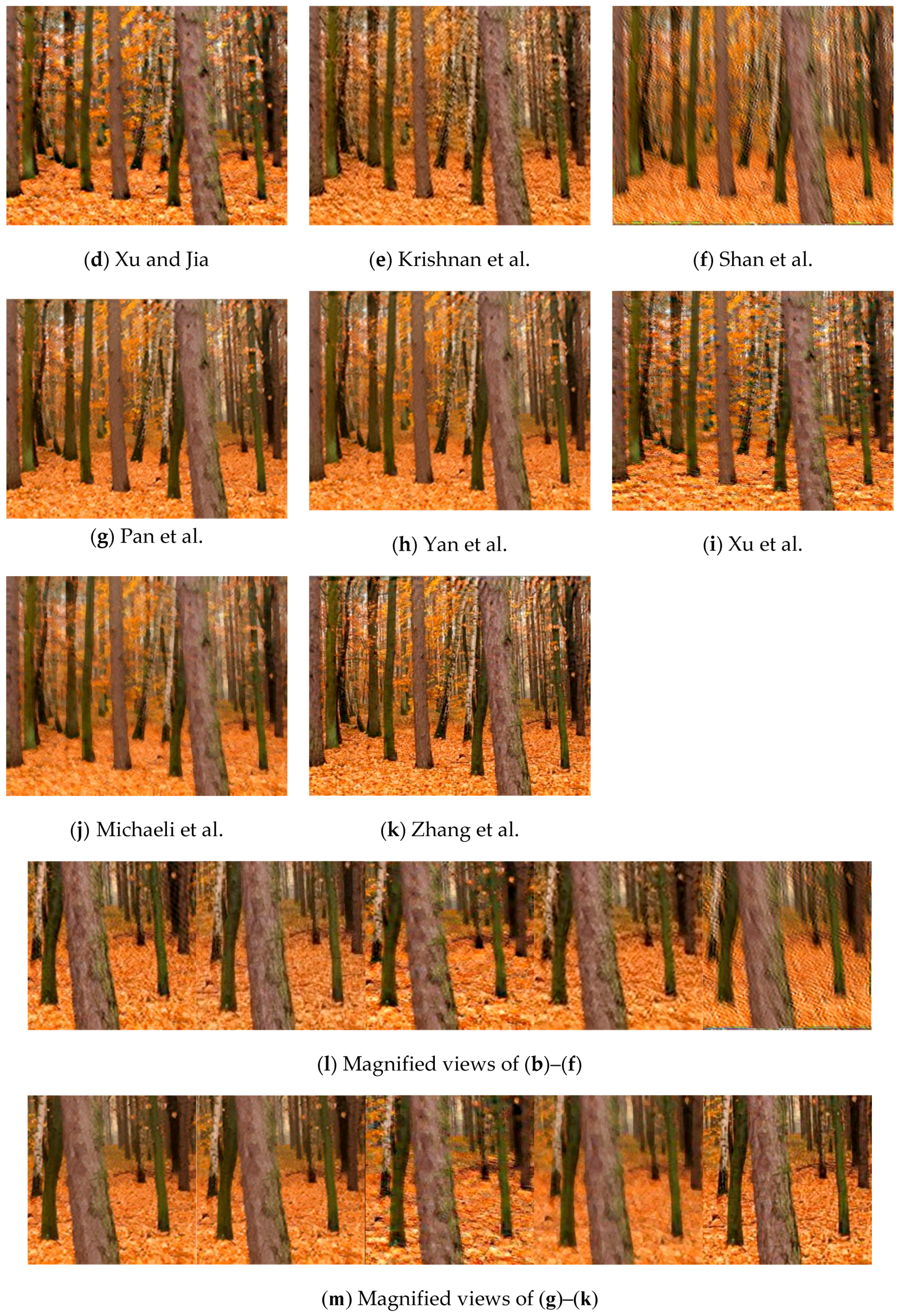
In addition, we test the performance based on the dataset of real captured standing trees, the ground truth images are shown in Figure 11. The images of living trees contain rich texture information, which are good typical images to test the results of deblurring. We obtain 32 blurred images based on the blurring kernels in Levin’s dataset and the four ground truths of images. The comparison methods include those in [7,9,19,20,22,27,30,31,36]. Figure 12 shows one of the results in the 32 blurring images. From the visualization results, the proposed method can reserve more texture information of an image compared with other methods—the image details can be seen clearly from the magnified views in Figure 12l,m. Figure 13 shows the average SSIM values and the success rate. The proposed method still has advantages over others—the SSIM are higher than others, and the success rate is the highest among the methods consistently.
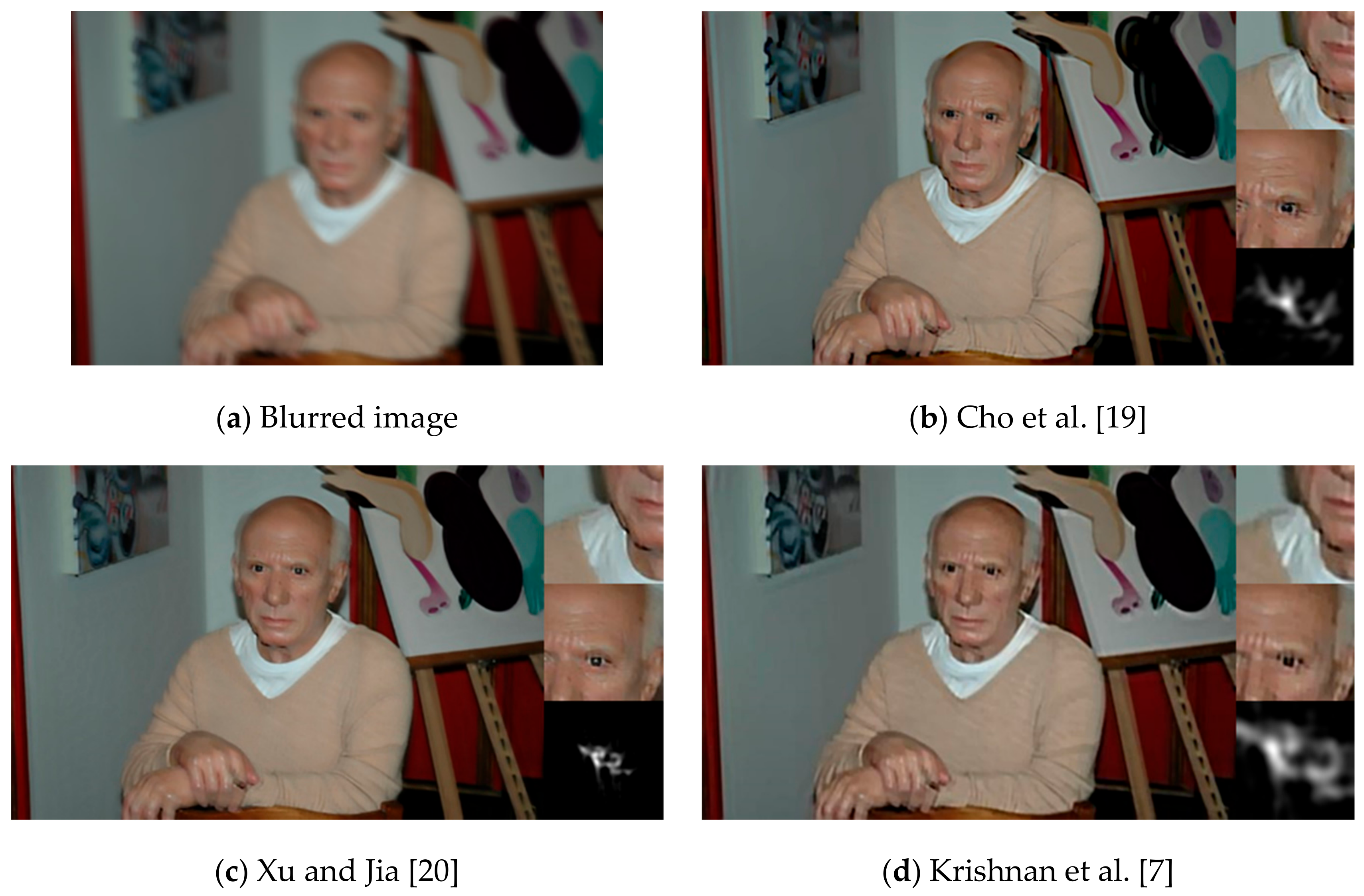
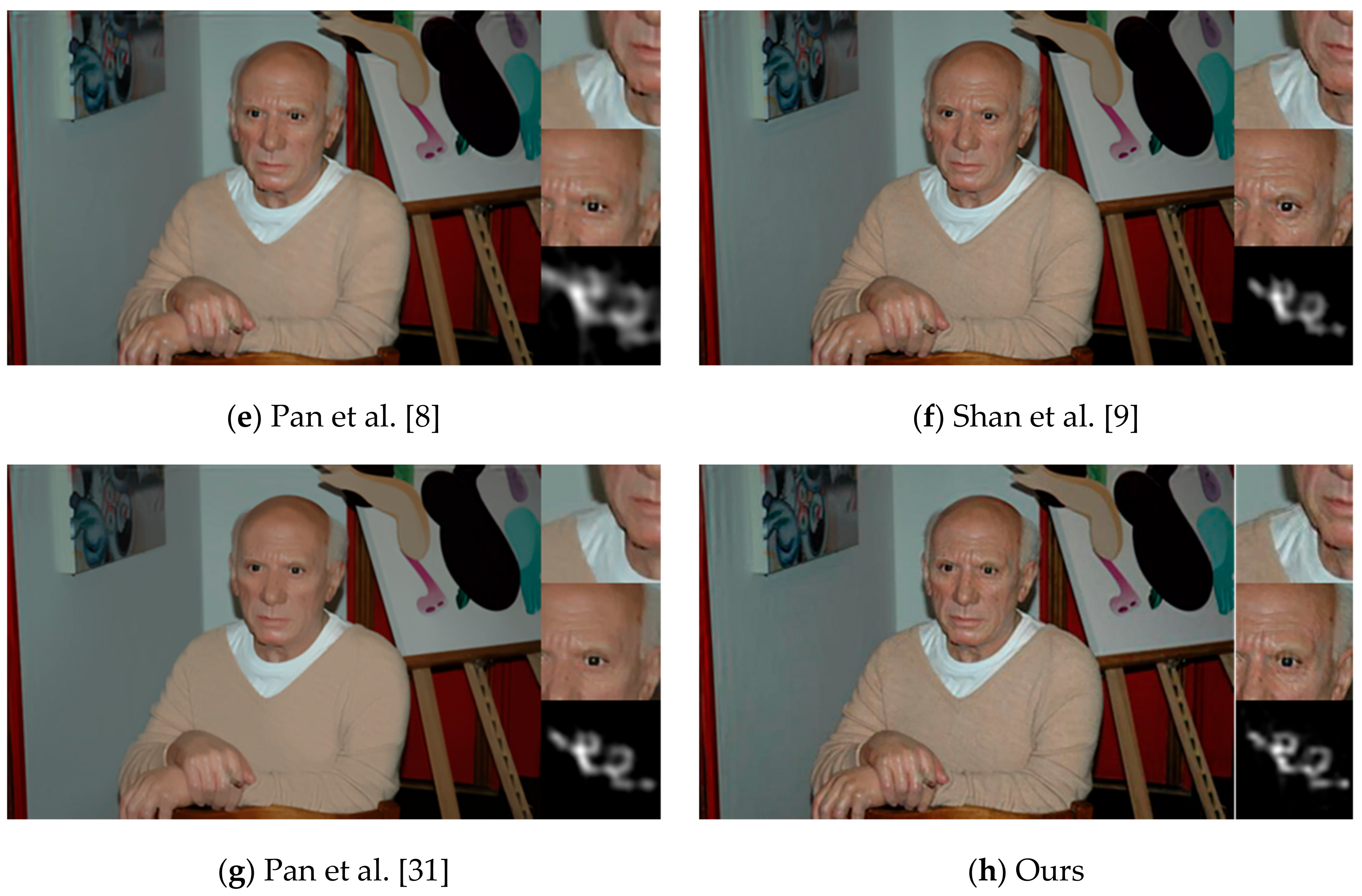
The experimental results also show that the proposed method can deblur natural blurred images well. In Figure 14, we compare the deblurring results for a natural blurred image with other methods. The clear image, their magnified views and the estimated blurring kernels are also shown together in the figure. Compared with other methods, the clear image obtained by the proposed method has fewer ringing artifacts, more image details and better color fidelity.
Figure 15 shows other blind deblurring results. The images are chosen from Xu’s dataset [20], Krishnan’s dataset [7], and the dataset of ours. Results show that the proposed method can deblur natural images well—the clear images have good color fidelity and clarity. The proposed method is effective in image blind deblurring.

4. Conclusions

In this paper, we propose a blind image deblurring method based on local edges selection. The proposed edges selection method based on local information is new and proven to be more effective than using global information when capturing images with dense structures, noise, and blur.
We use the new edges selection method to build the regularization term. Our model is simpler and more effective than other methods using image gradients. The image and blurring kernel are obtained simultaneously by alternating iteration. The experimental results show that the proposed blind deblurring method is effective for both gray value images and color images. Compared with other state-of-the-art deblurring methods, the quantitative results demonstrate the effectiveness of our method.
There are still some limitations of the proposed method. In the deblurring process of the proposed method, we assume that the blur is stationary, but in practical application, the blurring kernels are sometimes time-varying and space-varying, which are much more complex. We will further focus on the deblurring related to more complex blurring kernel in the future.

Author Contributions

Conceptualization, Y.H. and J.K.; methodology, Y.H.; software, Y.H.; validation, Y.H. and J.K.; formal analysis, Y.H.; investigation, Y.H.; resources, Y.H.; data curation, Y.H.; writing—original draft preparation, Y.H.; writing—review and editing, J.K.; visualization, J.K.; supervision, J.K.; project administration, J.K.; funding acquisition, J.K.

Funding

This work was supported by National Natural Science Foundation of China (Grant No. 31570713) and Beijing municipal construction project special fund.

Conflicts of Interest

The authors declare no conflict of interest.

References

  1. Whyte, O.; Sivic, J.; Zisserman, A. Deblurring shaken and partially saturated images. In Proceedings of the IEEE International Conference on Computer Vision Workshops, Barcelona, Spain, 6–13 November 2011; pp. 185–201. [Google Scholar]
  2. Krishnan, D.; Fergus, R. Fast image deconvolution using hyper-laplacian priors. In Advances in Neural Information Processing Systems 22, Proceedings of the 2009 Conference, Vancouver, BC, Canada, 7–10 December 2009; Curran Associates, Inc.: New York, NY, USA; pp. 1033–1041.
  3. Cho, S.; Wang, J.; Lee, S. Handling outliers in non-blind image deconvolution. In Proceedings of the International Conference on Computer Vision, Barcelona, Spain, 6–13 November 2011; pp. 495–502. [Google Scholar]
  4. Sun, L.; Cho, S.; Wang, J.; Hays, J. Edge-based blur kernel estimation using patch priors. In Proceedings of the IEEE International Conference on Computational Photography, Cambridge, MA, USA, 19–21 April 2013; pp. 1–8. [Google Scholar]
  5. Levin, A.; Weiss, Y.; Durand, F.; Freeman, W.T. Understanding and evaluating blind deconvolution algorithms. In Proceedings of the 2009 IEEE Conference on Computer Vision and Pattern Recognition (CNPR 2009), Miami, FL, USA, 20–25 June 2009; Volume 8, pp. 1964–1971. [Google Scholar]
  6. Mignotte, M. A non-local regularization strategy for image deconvolution. Pattern Recognit. Lett. 2008, 29, 2206–2212. [Google Scholar] [CrossRef]
  7. Krishnan, D.; Tay, T.; Fergus, R. Blind deconvolution using a normalized sparsity measure. In Proceedings of the IEEE Conference on Computer Vision and Pattern Recognitio, Colorado Springs, CO, USA, 20–25 June 2011; pp. 233–240. [Google Scholar]
  8. Pan, J.; Hu, Z.; Su, Z.; Yang, M.H. L0-regularized intensity and gradient prior for deblurring text images and beyond. IEEE Trans. Pattern Anal. Mach. Intell. 2017, 39, 342–355. [Google Scholar] [CrossRef] [PubMed]
  9. Qi, S.; Jia, J.; Agarwala, A. High-quality motion deblurring from a single image. ACM Trans. Graph. 2008, 27, 73. [Google Scholar]
  10. Mai, L.; Liu, F. Kernel fusion for better image deblurring. In Proceedings of the IEEE Conference on Computer Vision and Pattern Recognition, Boston, MA, USA, 7–12 June 2015; Volume 1, pp. 371–380. [Google Scholar]
  11. Levin, A.; Weiss, Y.; Durand, F.; Freeman, W.T. Efficient marginal likelihood optimization in blind deconvolution. In Proceedings of the IEEE Conference on Computer Vision & Pattern Recognition, Colorado Springs, CO, USA, 20–25 June 2011; pp. 2657–2664. [Google Scholar]
  12. Goldstein, A.; Fattal, R. Blur-kernel estimation from spectral irregularities. In Proceedings of the European Conference on Computer Vision, Florence, Italy, 7–13 October 2012; pp. 622–635. [Google Scholar]
  13. Cai, J.F.; Ji, H.; Liu, C.; Shen, Z. Blind motion deblurring from a single image using sparse approximation. In Proceedings of the IEEE Conference on Computer Vision & Pattern Recognition, Miami, FL, USA, 20–25 June 2009; pp. 104–111. [Google Scholar]
  14. Almeida, M.S.C. Blind and semi-blind deblurring of natural images. IEEE Trans. Image Process. 2010, 19, 36–52. [Google Scholar] [CrossRef] [PubMed]
  15. Joshi, N.; Szeliski, R.; Kriegman, D.J. Psf estimation using sharp edge prediction. In Proceedings of the IEEE Conference on Computer Vision & Pattern Recognition, Anchorage, AK, USA, 23–28 June 2008; pp. 24–26. [Google Scholar]
  16. Jia, J. Single image motion deblurring using transparency. In Proceedings of the IEEE Conference on Computer Vision & Pattern Recognition, Minneapolis, MN, USA, 17–22 June 2007. [Google Scholar]
  17. Zhe, H.; Yang, M.H. Good regions to deblur. In Proceedings of the European Conference on Computer Vision, Florence, Italy, 7–13 October 2012; pp. 59–72. [Google Scholar]
  18. Javaran, T.A.; Hassanpour, H.; Abolghasemi, V. Local motion deblurring using an effective image prior based on both the first- and second-order gradients. Mach. Vis. Appl. 2017, 28, 431–444. [Google Scholar]
  19. Cho, S.; Lee, S. Fast motion deblurring. In Proceedings of the Acm Siggraph Asia, Yokohama, Japan, 16–19 December 2009; p. 145. [Google Scholar]
  20. Xu, J.J.L. Two-phase kernel estimation for robust motion deblurring. In Proceedings of the European Conference on Computer Vision—ECCV, Heraklion, Greece, 5–11 September 2010; pp. 157–170. [Google Scholar]
  21. Han, Y.; Kan, J. Blind color-image deblurring based on color image gradients. Signal Process. 2019, 155, 14–24. [Google Scholar] [CrossRef]
  22. Zhang, K.; Zuo, W.; Gu, S.; Zhang, L. Learning deep cnn denoiser prior for image restoration. In Proceedings of the 2017 IEEE Conference on Computer Vision and Pattern Recognition (CVPR), Honolulu, HI, USA, 21–26 July 2017; Volume 1, pp. 2808–2817. [Google Scholar]
  23. Xu, L.; Ren, J.S.J.; Liu, C.; Jia, J. Deep convolutional neural network for image deconvolution. In Proceedings of the 27th International Conference on Neural Information Processing Systems, Montreal, QC, Canada, 8–13 December 2014; Volume 1, pp. 1790–1798. [Google Scholar]
  24. Ghosh, D.; Xiong, F.; Sirsi, S.R.; Shaul, P.W.; Mattrey, R.F.; Hoyt, K. Toward optimization of in vivo super-resolution ultrasound imaging using size-selected microbubble contrast agents. Med. Phys. 2017, 44, 6304–6313. [Google Scholar] [CrossRef] [PubMed]
  25. Ghosh, D.; Kaabouch, N.; Hu, W.-C. A robust iterative super-resolution mosaicking algorithm using an adaptive and directional huber-markov regularization. J. Vis. Commun. Image Represent. 2016, 40, 98–110. [Google Scholar] [CrossRef]
  26. Ghosh, D.; Peng, J.; Brown, K.; Sirsi, S.; Mineo, C.; Shaul, P.W.; Hoyt, K. Super-resolution ultrasound imaging of skeletal muscle microvascular dysfunction in an animal model of type 2 diabetes. J. Ultrasound Med. 2019. [Google Scholar] [CrossRef] [PubMed]
  27. Michaeli, T.; Irani, M. Blind deblurring using internal patch recurrence. In Proceedings of the European Conference on Computer Vision, Zurich, Switzerland, 6–12 September 2014; pp. 783–798. [Google Scholar]
  28. Danielyan, A.; Katkovnik, V.; Egiazarian, K. Bm3d frames and variational image deblurring. IEEE Trans. Image Process. 2012, 21, 1715–1728. [Google Scholar] [CrossRef] [PubMed]
  29. He, K.; Jian, S.; Tang, X. Single image haze removal using dark channel prior. In Proceedings of the IEEE Conference on Computer Vision & Pattern Recognition, Miami, FL, USA, 20–25 June 2009; pp. 1956–1963. [Google Scholar]
  30. Yan, Y.; Ren, W.; Guo, Y.; Rui, W.; Cao, X. Image deblurring via extreme channels prior. In Proceedings of the IEEE Conference on Computer Vision & Pattern Recognition, Honolulu, HI, USA, 21–26 July 2017; pp. 6978–6986. [Google Scholar]
  31. Pan, J.; Sun, D.; Pfister, H.; Yang, M.H. Blind image deblurring using dark channel prior. In Proceedings of the Computer Vision & Pattern Recognition, Las Vegas, NV, USA, 27–30 June 2016; pp. 1628–1636. [Google Scholar]
  32. Almeida, M.S.C.; Figueiredo, M.A.T. Blind image deblurring with unknown boundaries using the alternating direction method of multipliers. In Proceedings of the IEEE International Conference on Image Processing, Melbourne, Australia, 15–18 September 2013; pp. 586–590. [Google Scholar]
  33. Perrone, D.; Favaro, P. Total variation blind deconvolution: The devil is in the details. In Proceedings of the IEEE Conference on Computer Vision & Pattern Recognition, Zurich, Switzerland, 6–12 September 2014; pp. 2909–2916. [Google Scholar]
  34. Paul, B.; Lei, Z.; Xiaolin, W. Canny edge detection enhancement by scale multiplication. IEEE Trans. Pattern Anal. Mach. Intell. 2005, 27, 1485–1490. [Google Scholar] [Green Version]
  35. Almeida, M.S.C.; Figueiredo, M.A.T. New stopping criteria for iterative blind image deblurring based on residual whiteness measures. In Proceedings of the IEEE Statistical Signal Processing Workshop, Nice, France, 28–30 June 2011; pp. 337–340. [Google Scholar]
  36. Li, X.; Zheng, S.; Jia, J. Unnatural l0 sparse representation for natural image deblurring. In Proceedings of the IEEE Conference on Computer Vision & Pattern Recognition, Portland, OR, USA, 23–28 June 2013; pp. 1107–1114. [Google Scholar]
  37. Zhou, W.; Alan Conrad, B.; Hamid Rahim, S.; Simoncelli, E.P. Image quality assessment: From error visibility to structural similarity. IEEE Trans. Image Process. 2004, 13, 600–612. [Google Scholar]
  38. Ghosh, D.; Park, S.; Kaabouch, N.; Semke, W. Quantitative evaluation of image mosaicing in multiple scene categories. In Proceedings of the 2012 IEEE International Conference on Electro/Information Technology, Indianapolis, IN, USA, 6–8 May 2012; pp. 1–6. [Google Scholar]
  39. Köhler, R.; Hirsch, M.; Mohler, B.; Schölkopf, B.; Harmeling, S. Recording and playback of camera shake: Benchmarking blind deconvolution with a real-world database. In Proceedings of the European Conference on Computer Vision, Florence, Italy, 7–13 October 2012; pp. 27–40. [Google Scholar]
  40. Hirsch, M.; Schuler, C.J.; Harmeling, S.; Schölkopf, B. Fast removal of non-uniform camera shake. In Proceedings of the IEEE International Conference on Computer Vision, Barcelona, Spain, 6–13 November 2011; pp. 1439–1451. [Google Scholar]
  41. Fergus, R. Removing camera shake from a single photograph. ACM Trans. Graph. 2006, 25, 787–794. [Google Scholar] [CrossRef]
  42. Li, L.; Pan, J.; Lai, W.S.; Gao, C.; Yang, M.H. Learning a discriminative prior for blind image deblurring. In Proceedings of the 2017 IEEE International Conference on Computer Vision, Salt Lake City, UT, USA, 18–23 June 2018; pp. 1077–1085. [Google Scholar]
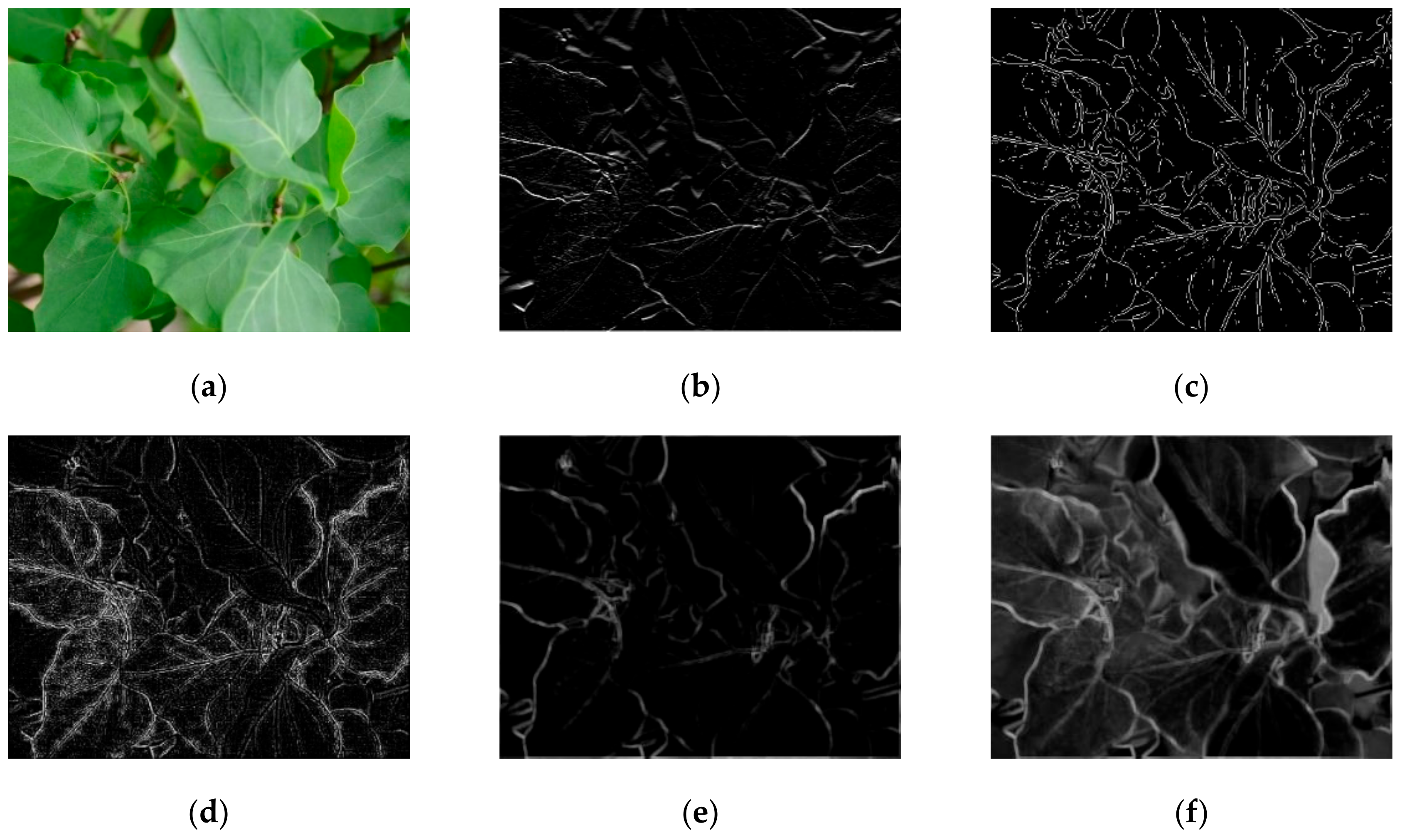
Figure 1. Comparison of different edges selection method: (a) Original image, (b) first-order gradients of image, (c) edges extracted by Canny operator, (d) Laplace gradients, (e) local edges of gray value image obtained by the proposed method, (f) local edges of color image obtained by the proposed method.
Applsci 09 03274 g001
Figure 2. Image edges comparison of blurred image (from left to right are clear image, blurred image, horizontal first-order gradients, vertical first-order gradients, second-order gradients, edges extracted by Canny operator, Laplace gradients, local edges of gray image, and local edges of color image).
Applsci 09 03274 g002
Figure 3. (a) Clear image, (b) edges selected with the window size = 5 × 5, (c) edges selected with the window size = 7 × 7, (d) edges selected with the window size = 9 × 9, (e) blurred image, (f) deblurring result with the window size = 5 × 5, (g) deblurring result with the window size = 7 × 7, (h) deblurring result with the window size = 9 × 9.
Applsci 09 03274 g003
Figure 4. Sensitivity analysis of α and β . (a) The sensitivity analysis of α ; (b) the sensitivity analysis of β .
Applsci 09 03274 g004
Figure 5. The convergence of the proposed method: (a) the convergence of image, and (b) the convergence of blurring kernel.
Applsci 09 03274 g005
Figure 6. Levin’s dataset.
Applsci 09 03274 g006
Figure 7. The deblurring results of Levin’s dataset.
Applsci 09 03274 g007aApplsci 09 03274 g007b
Figure 8. Quantitative results on the dataset of Levin et al.
Applsci 09 03274 g008aApplsci 09 03274 g008b
Figure 9. Image deblurring results on the dataset of Köhler et al.
Applsci 09 03274 g009
Figure 10. The quantitative results on the dataset of Köhler et al.
Applsci 09 03274 g010
Figure 11. Ground truth images of standing trees.
Applsci 09 03274 g011
Figure 12. Image deblurring results of standing trees.
Applsci 09 03274 g012aApplsci 09 03274 g012b
Figure 13. Image deblurring performance of living standing trees.
Applsci 09 03274 g013
Figure 14. The deblurring results comparison of natural blurred image.
Applsci 09 03274 g014aApplsci 09 03274 g014b
Figure 15. The deblurring results of natural images.
Applsci 09 03274 g015aApplsci 09 03274 g015b
Table 1. Quantitative comparison of the deblurring results in Figure 7.
SSIMPSNRKS
Cho et al.0.48528.570.556
Xu and Jia0.78926.530.623
Krishnan et al.0.65431.690.583
Shan et al.0.69730.770.633
Pan et al.0.80031.720.699
Perrone et al.0.73226.860.691
Xu et al.0.58826.330.621
Michaeli et al.0.62430.100.612
Zhang et al.0.76930.530.705
Ours0.82331.820.713